Radiation-magnetohydrodynamic simulations of H ii regions and their associated PDRs in turbulent molecular clouds Free

Abstract

1 INTRODUCTION

H ii regions, that is, regions of photoionized gas, are among the most arresting astronomical objects at optical wavelengths. The basic theory behind their formation and expansion has been known for some time (Strömgren 1939; Kahn 1954; Spitzer 1978). More recently, attention has turned to explaining the irregular structures, filaments, globules and clumps seen within and around these regions. These could be due to underlying density inhomogeneities in the molecular cloud into which the H ii region is expanding or could be due to instabilities at the ionization front itself (Garcia-Segura & Franco 1996; Williams, Ward-Thompson & Whitworth 2001; Mellema et al. 2006a; Gritschneder et al. 2010; Mackey & Lim 2010). The effect of the stellar ionizing radiation on these structures can lead to radiation-driven implosion, and the subsequent compression could result in the formation of new stars (Bertoldi 1989; Esquivel & Raga 2007; Motoyama, Umemoto & Shang 2007).

Magnetic fields are well known to pervade molecular clouds and are thought to play an important role in regulating the star formation process by providing support to collapsing structures in molecular clouds (Mouschovias & Ciolek 1999), although recently their relative importance in this process has become less clear (McKee & Ostriker 2007). However, theoretical work on the interplay between ionizing radiation and magnetic fields in and around H ii regions has only been possible recently, with the advent of radiation-magnetohydrodynamic (MHD) codes. Krumholz, Stone & Gardiner (2007) performed the first simulations of the expansion of an H ii region in a uniform, magnetized medium. At early times, the thermal pressure of the photoionized gas dominates over the magnetic field, which is pushed out of the expanding H ii region. At late times (several Myr), the photoionized region becomes elongated along the field lines and the magnetic field filled back in. Henney et al. (2009) and Mackey & Lim (2011) have studied the effects of ionizing radiation on magnetized globules, finding that the photoevaporation process is significantly altered only when the magnetic pressure exceeds the thermal pressure by more than a factor of 10 in the initial globule. Peters et al. (2011) have recently studied the combined effects of magnetic fields and photoionization on the formation of a massive star on scales of <0.1 pc, finding that rotational winding of the field lines produces a magnetized ‘bubble’, whose magnetic pressure acts to confine the nascent H ii region during its ultracompact phase.

In this paper, we study the expansion of H ii regions in non-uniform (turbulent) magnetized molecular clouds. Previously, we studied H ii region expansion in a turbulent medium without a magnetic field and our results were strikingly similar to observed H ii regions (Mellema et al. 2006a). In this work, we study the effect of the expanding photoionized gas on structures in the surrounding magnetized medium and also the effect that the turbulent magnetic field has on the H ii region itself. At least at the relatively early times studied in our simulations, most of the interesting effects due to the magnetic field will occur within the neutral, photon-dominated region around the H ii region, and so we use a careful treatment of the heating and cooling processes in this gas, first discussed in Henney et al. (2009), in order to have a realistic portrayal of the dynamical processes here.

The wealth of new observational data at infrared wavelengths enables comparisons to be made of our simulations not only with observations of the photoionized gas, as done previously in Mellema et al. (2006a), but also with the photodissociation region (PDR) and molecular gas affected by the H ii region. In particular, the Spitzer GLIMPSE surveys of bubbles in the Galactic plane (Churchwell et al. 2006, 2007) highlight polycyclic aromatic hydrocarbon (PAH) emission at the outer edges of H ii regions and in PDRs. These surveys show that the thickness of the PAH-emitting shell varies between 0.2 and 0.4 of the outer radius and that shell thickness increases approximately linearly with radius. Moreover, the bubbles are generally non-spherical. Herschel and APEX observations reveal thermal emission from cold dust in the molecular gas outside the PDR (e.g. Anderson et al. 2010; Deharveng et al. 2010). These observations are useful in identifying condensations that could be collapsing to form new stars.

Studies of magnetic fields in and around molecular clouds are important for understanding the star formation process. There is no consensus as to the importance of magnetic fields in the formation of clouds, cores and ultimately stars. If magnetic fields are dynamically important, then star formation is regulated by ambipolar diffusion (e.g. Mouschovias & Ciolek 1999). Alternatively, if magnetic fields are unimportant then other processes such as turbulence and stellar feedback provide support to molecular clouds and determine the star formation efficiency (e.g. Ballesteros-Paredes, Vázquez-Semadeni & Scalo 1999; Elmegreen 2000; Matzner 2002; Krumholz, Matzner & McKee 2006; Tasker & Tan 2009; Tasker 2011). It is not known whether magnetic fields are strong enough to dynamically support molecular clouds and more evidence is needed. It is possible that reality lies somewhere between these extremes. Recent Zeeman observations of molecular clouds (Crutcher, Hakobian & Troland 2009; Crutcher et al. 2010) do not agree with predictions of idealized ambipolar diffusion models (strong magnetic field), but more observations are needed.

There are three main techniques for tracing the magnetic field in diffuse H i and molecular clouds: polarization from aligned dust grains, linear polarization of spectral lines and Zeeman splitting of spectral lines (Heiles & Crutcher 2005). Polarization studies yield B_⊥, the strength of the field projected on to the plane of the sky, whereas Zeeman splitting gives B_||, the strength of the field parallel to the line of sight. In particular, the H i Zeeman effect has been used to study the atomic gas (assumed to be in the photodissociated region) in the star-forming regions M17 (Brogan & Troland 2001) and the Ophiuchus dark cloud complex (Goodman & Heiles 1994), while the OH Zeeman effect is used to study the line-of-sight magnetic field in the molecular gas. The results of such studies suggest that there is rough equipartition of magnetic and turbulent (dynamical) energy densities in the neutral gas. In the Ophiuchus dark cloud region, the uniform field in the H i gas is estimated to be 10.2 μG (Goodman & Heiles 1994), whereas the magnitude of the line-of-sight magnetic field strength in the H i gas associated with M17 is found to be ∼ 500 μG (at 60 − arcsec resolution or even twice as high at 26 − arcsec resolution; Brogan & Troland 2001), suggesting that there is small-scale structure in the magnetic field. Recent linear polarization studies at submillimetre wavelengths of the magnetic field around the ultracompact H ii region G5.89–0.39 (Tang et al. 2009) provide evidence for compression of the B field in the surrounding molecular cloud and general disturbance of the magnetic field caused by the expansion of the H ii region.

For photoionized gas, Faraday rotation measures of line-of-sight extragalactic radio sources are used to calculate the magnetic field strengths in foreground H ii regions (Heiles, Chu & Troland 1981). The Zeeman effect cannot be used in the ionized gas because the thermal linewidths are too large. Heiles et al. (1981) used double extragalactic radio sources to sample two positions in the H ii regions S117 and S264 and found identical rotation measures in each case of the order of 1 or 2 μG. In these regions, the thermal energy density dominates the magnetic energy density. In a third H ii region, S119, for which only a single rotation measure is available, the line-of-sight magnetic field strength is around 20 μG and the ratio of magnetic to thermal energy density is around 0.4; hence, the magnetic field could have had an effect on the expansion of this H ii region.

The remainder of this paper is organized as follows. In Section 2, we describe our numerical algorithm and present two test problems as follows. First, the classical Spitzer law for the expansion of a non-magnetized H ii region in a uniform medium and secondly, the expansion of an H ii region in a uniform magnetized medium (Krumholz et al. 2007; Mackey & Lim 2011) are discussed. In the second problem, we draw attention to some interesting properties of the solution that have not been described previously.

In Section 3 we describe the expansion of H ii regions in both magnetized and non-magnetized turbulent media, taking as initial conditions for the ambient medium the results of an MHD turbulence calculation (Vázquez-Semadeni et al. 2005) and considering both a strong (approximately O9 spectral type) ionizing source and a weak (B0.5) one. In Section 4, we make qualitative comparisons between simulated optical and long-wavelength images and observations. We also produce synthetic maps of the projected line-of-sight and plane-of-sky components of the magnetic field, which can be qualitatively compared with observations of the magnetic field in star-forming regions. We discuss the globules and filaments at the periphery of our simulated H ii regions in the context of recent numerical work on photoionized magnetized globules (Henney et al. 2009; Mackey & Lim 2011). Finally, in Section 5, we outline our conclusions.

2 NUMERICAL MODEL

2.1 Numerical method

The numerical method used in this paper is the same as that described by Henney et al. (2009). The phab-c² code combines the ideal MHD code described by De Colle & Raga (2006) with the conservative causal ray (C²-Ray) method for radiative transfer developed by Mellema et al. (2006b) and adds a new treatment of the heating and cooling in the neutral gas (Henney et al. 2009). The MHD code is a second-order upwind scheme that integrates the ideal MHD equations using a Godunov method with a Riemann solver, similar to that described by Falle, Komissarov & Joarder (1998) but with the constrained transport method (e.g. Tóth 2000) used to maintain the divergence of the magnetic field close to zero. An artificial (Lapidus) viscosity is also included (Colella & Woodward 1984) in order to broaden the discontinuities and reduce oscillations. The C²-Ray method for radiative transfer is explicitly photon conserving (Mellema et al. 2006b) and the algorithm allows for time-steps much longer than the characteristic ionization time-scales or the time-scale for the ionization front to cross a numerical grid cell, by means of an analytical relaxation solution for the ionization rate equations. This results in a highly efficient radiative transfer method.

The MHD and radiative transfer codes are coupled via operator splitting, the inclusion of equations for the advection of ionized and neutral density in the MHD code and the energy equation, which includes both radiative cooling and heating due to the absorption of stellar radiation by gas or dust: ionizing extreme ultraviolet (EUV) radiation in the photoionized region, non-ionizing far-ultraviolet (FUV) radiation in the neutral gas and X-rays in the dense molecular gas. A detailed discussion of the heating and cooling contributions is given by Henney et al. (2009). In particular, the treatment of heating in the neutral PDR region, taking into account FUV/optical dust heating and X-ray heating, is a substantial improvement over standard treatments in the literature. The heating term for the neutral gas is calibrated using cloudy (Ferland et al. 1998) and is tailored to the ionization source. Moreover, X-rays and FUV radiation will be enhanced due to the presence of associated low-mass stars in the star formation environment, and we use the results of Fatuzzo & Adams (2008) to estimate the distributions of FUV and EUV fluxes appropriate to stellar clusters of membership sizes relevant to the two cases we study: an O9 and a B0.5 star. The energy equation is solved iteratively using substepping, and the time-step for the whole calculation is determined solely by the MHD time-step.

The individual components of the phab-c² code have been tested against standard problems (De Colle & Raga 2004; De Colle 2005; Iliev et al. 2006) and the whole code was applied to the problem of the photoionization of magnetized globules in Henney et al. (2009), work which has recently been independently corroborated by Mackey & Lim (2011). In this paper, we have implemented an entropy fix (Balsara & Spicer 1999) to correctly deal with the thermal and dynamical pressures in regions of low density where the magnetic pressure dominates. We have also improved the treatment of the boundary conditions because they can become important, particularly towards the end of the simulations. For our O-star simulations we use outflow boundary conditions, since thermal pressure is expected to dominate throughout the evolution and the H ii region will rapidly grow to the size of the computational box. For the B-star simulations, the expansion time-scale of the H ii region is much longer and is comparable to the crossing time of the computational box corresponding to the initial turbulent velocity dispersion of the molecular gas. We therefore use periodic boundary conditions in this case, which ensure that the total mass in the computational box remains constant.

Parallelization using Open-MP was implemented where possible, enabling the current simulations to be run in about 2 weeks on an Intel 8-core server with 32 GB of RAM. Preliminary work was performed on the Kan Balam supercomputer of the Universidad Nacional Autónoma de México.

2.2 Test problems

2.2.1 Hydrodynamic H ii region expansion in a uniform medium

The radiation part of the code has been extensively tested and documented (Iliev et al. 2006; Mellema et al. 2006b). In order to test the radiation (magneto-)hydrodynamics combined code, we first consider the purely hydrodynamic (HD) evolution of a photoionized region around an ionizing source in a uniform medium. The analytical solution to this problem is the familiar Spitzer (1978) expansion law:

1

where R_Spitzer is the ionization front radius, R₀ = (3 Q_H/4πn²₀α_B)^1/3 is the initial Strömgren radius, c_i is the sound speed in the ionized gas and t is the time, Q_H is the ionizing photon rate, n₀ is the ambient density and α_B is the case B recombination rate, α_B = 2.6 × 10⁻¹³T^−0.7 (Osterbrock & Ferland 2006), where T is the temperature in the ionized gas. For an ambient density n₀ = 1000 cm⁻³, stellar ionizing photon rate Q_H = 5 × 10⁴⁶ s⁻¹ and stellar temperature T_eff = 37 500 K, the results are shown in Fig. 1, together with the corresponding analytic solution. These parameters were chosen because they represent the mean values of the turbulent medium B-star case described below in Section 3. The top panel shows radius against time, while the bottom panel shows the relative error, defined as

2

From this figure, we see that the largest discrepancies, of about 6 per cent, occur at the beginning of the expansion, when a shock wave begins to propagate outwards ahead of the ionization front and a corresponding rarefaction wave travels back towards the ionizing source, which is not accounted for in the analytical solution. At later times, the error is never more than 1 per cent. Our code therefore compares extremely favourably with other radiation-HD codes on this problem (see e.g. Arthur & Hoare 2006; Krumholz et al. 2007; Iliev et al. 2009). There is no evidence for overcooling in the ionization front in our simulations, as was found to be a problem by Krumholz et al. (2007). In the analytic Spitzer solution, we assume an H ii region temperature T = 8900 K, which gives the best fit to our numerical result. This is about 400 K hotter than the volume-averaged ionized gas temperature in our simulation, but is roughly equal to the ionized gas temperature just inside the ionization front.

Figure 1

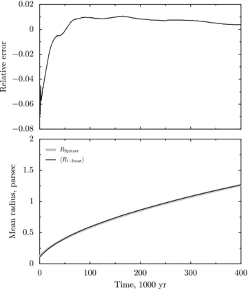
Radius against time for the HD expansion of a photoionized region in a uniform medium. Bottom panel: numerical simulation (black line) and analytical solution (grey line). Top panel: relative error.

Open in new tabDownload slide

In Fig. 2, we plot the gas radial velocity from the numerical simulation and the corresponding analytical solution. The numerical solution closely follows the analytical solution, though with oscillations due to acoustic phenomena, such as the initial rarefaction wave, which propagates back into the H ii region when the ionization front begins to expand outwards.

Figure 2

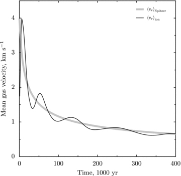
Mean gas velocity against time for the HD expansion of a photoionized region in a uniform medium. Black line: numerical simulation; thick grey line: analytic solution.

Open in new tabDownload slide

2.2.2 MHD H ii region expansion

There is no corresponding analytical solution for the expansion of an H ii region into a magnetized medium. Therefore, in order to test the MHD part of the numerical code, we carry out a simulation of the expansion of an H ii region in a uniform magnetized medium using the same parameters as those of Krumholz et al. (2007). This problem was also used to test the radiation MHD code of Mackey & Lim (2011). The simulation is performed in a 256³ computational box with a constant ambient density and temperature of n₀ = 10² cm⁻³ and T₀ = 11 K, respectively, a constant ambient magnetic field directed at 30° to the x-axis in the x–y plane¹ of strength B₀ = 14.2 μG and an ionizing source producing Q_H = 4 × 10⁴⁶ ionizing photons s⁻¹. The magnetic field is placed at an angle to the grid lines in order to be able to distinguish between physical and computational effects. We run the simulation in a (20 pc)³ and (40 pc)³ box, the former to study the early evolution (t < 2 Myr) and the latter to highlight the late-time evolution. We note that the ionizing source is very weak (later than spectral type B0.5; Vacca, Garmany & Shull 1996) and that the ambient density is lower than that typically found in star-forming regions.

Krumholz et al. (2007) found a critical radius and time for when magnetic pressure and tension start to become important for the expansion of the H ii region in a uniform magnetized medium, which corresponds to when the magnetic pressure in the neutral gas becomes of the same order as the thermal pressure in the ionized gas, i.e. ρ_nv²_A∼ρ_ic_i². Here, ρ_n and ρ_i are, respectively, the densities in the neutral and ionized gas, v_A is the Alfvén speed and c_i is the sound speed in the ionized gas. Thus, magnetic effects become significant when the H ii region has expanded to a radius of roughly

3

where R₀ is the initial Strömgren radius in a non-magnetized medium of the same uniform density. The corresponding time is

4

where t₀ is the sound-crossing time of the initial Strömgren sphere, and both of these equations implicitly assume that the classical Spitzer expansion law (Spitzer 1978) holds until the magnetic field becomes important.

For the parameters in this test problem, the initial Strömgren radius is R₀ = 0.48 pc and the Alfvén speed in the ambient magnetized medium is 2.6 km s⁻¹. Our simulations give a temperature in the photoionized gas of T_i∼ 9000 K and hence a sound speed of c_i = 9.8 km s⁻¹ [compare the lower assumed ionized sound speed c_i∼ 8.7 km s⁻¹ in the Krumholz et al. (2007) models]. Thus, the critical radius and time are R_m = 2.8 pc and t_m = 0.61 Myr, respectively, for our models.

In Figs 3 and 4, we show snapshots of the magnetic field and the photoionized gas distribution in the central x–y, x–z and y–z planes of the computational box after 2 and 6 Myr of evolution. The coloured discs shown between the panels of the top row are keys to the interpretation of the magnetic field images. The hue indicates the projected field orientation in the plane of each cut (red for vertical, cyan for horizontal, etc.), while the brightness indicates the magnetic field strength, as is shown in the left-hand disc. The colour saturation diminishes as the out-of-plane component of the field increases, as shown in the right-hand disc. This non-standard representation allows the magnetic field to be sampled at every pixel. The bottom panels of the figures show the ionization fraction, temperature and density of the gas in the same central planes. Ionization fraction is represented by colour: red indicates fully ionized gas while blue/green is partially ionized. The gas temperature varies between ∼10⁴ K (red) in the ionized gas to a few hundred Kelvin in the neutral (PDR) gas. The gas density is represented by the intensity in these figures, with the densest, cold molecular gas appearing white.

Figure 3

Expansion of an H ii region in a magnetized uniform medium after 2 Myr in a (20 pc)³ computational box. The top row shows the magnetic field in cuts in the central x–y (left), x–z (centre) and y–z (right) planes. The colour indicates the direction of the magnetic field, where the coloured discs show the field angle in the plane for a strong field (left, brighter disc) and a weaker field (right, dimmer disc). Grey indicates a magnetic field perpendicular to the plane. The bottom row shows ionization fraction x, temperature T and density ρ, coded as ‘hue’, ‘saturation’ and ‘value’, respectively. Red indicates hot (∼10⁴ K) ionized gas, blue/green is partially ionized gas, purple is warm (∼300 K) neutral (PDR) gas and grey indicates cold neutral (molecular) gas. The density is represented by the intensity, with the densest gas being white and the most diffuse being black.

Open in new tabDownload slide

Figure 4

Same as Fig. 3 but after 6 Myr in a (40 pc)³ computational box.

Open in new tabDownload slide

At early times, t < t_m, the H ii region is essentially spherical and expands at approximately the same speed (half the sound speed) in all directions because the ionized gas thermal pressure is much higher than the ambient magnetic pressure. Expansion across the magnetic field lines compresses the B field. The expanding H ii region and PDR are preceded by a fast-mode shock, which travels furthest perpendicular to the magnetic field direction. The fast-mode shock bends and compresses the field lines and so the PDR and H ii region propagate in a modified magnetic field. The slow-mode shock is strongest along the field lines and most evident at the end caps, where it produces a dense shell. It compresses the gas and demagnetizes it (reduces the field). The slow-mode shock is almost isothermal and the dense shell behind it is pushed by the pressure in the photoionized region. At early times, the magnetic field is reduced in the photoionized gas by the expansion of the H ii region. At later times, t > t_m, the magnetic tension pulls the field back into the H ii region at the equator.

In Fig. 3 we show the situation after 2 Myr, when the magnetic field has started to pull back into the H ii region. The H ii region is elongated along the magnetic field direction but the photon-dominated region (warm neutral gas) is approximately spherical. The magnetic field retains its original direction except around the edge of the H ii region. This is particularly evident at the poles of the H ii region. At the time shown in the figure, the magnetic field appears concentrated towards the centre, with regions of a lower magnetic field around the equator or waist of the structure. Neutral gas is pulled into the H ii region along with the magnetic field, becomes ionized and flows away from the ionization front into the H ii region. It then flows along the field lines and is channelled out towards the poles, where the ionization front transforms into a recombination front. We note that at this time in the simulation, we do see instabilities form in the direction perpendicular to the magnetic field, as reported by Krumholz et al. (2007) and Mackey & Lim (2011). These instabilities form at the equator where the ionization front is parallel to the magnetic field direction because the slow-mode shock which precedes the ionization front is not permitted to cross the field lines. As a result, the ionization front corrugates.

Fig. 4 shows the simulation after 6 Myr in a (40 pc)³ computational box. The H ii region has stopped expanding perpendicular to the magnetic field but the shocked neutral shell is still expanding along the field lines, leading to a very elongated structure. However, in the direction along the field lines, the flow has become one dimensional and so the density does not fall off as the H ii region expands. Thus, there is a limit as to how far the ionization/recombination front can travel in this direction. There is an extended region of partially ionized gas beyond the recombination front. The warm, neutral gas (PDR) is still roughly spherical in shape but is pierced by the cigar-shaped H ii region along the field direction. The dense neutral knots formed as a result of the instability at the equator shadow parts of the PDR. The knots formed closest to the perpendicular direction remain there throughout the simulation, pinned by the magnetic field. The knots slightly off the equator experience the rocket effect due to the photoionization of their outer skins. They move like beads on a wire along the magnetic field lines around the edge of the H ii region, a process which can be clearly observed in animations of this simulation. By the end of the calculation, the magnetic field has refilled the H ii region and become roughly uniform and returned completely to its original direction.

Finally, in Figs 5 and 6, we examine the expansion of the magnetized H ii region. Fig. 5 shows the evolution of the radius of the photoionized region with time. The mean radius is consistently below the classical Spitzer expansion law, unlike the non-magnetic case (see Fig. 1). In the direction perpendicular to the magnetic field, the expansion slows with time, as shown by the evolution of the minimum radius. In the direction along the field lines, the expansion initially (t≤ 1 Myr) follows the classical Spitzer law but then accelerates as material is channelled along the field lines and out of the poles of the H ii region. This expansion abruptly stops just after 4 Myr, which corresponds to the time when the ionization front can no longer expand along the field lines because the flow has become one dimensional.

Figure 5

Radius against time for the MHD expansion of a photoionized region in a uniform magnetized medium. Numerical MHD simulation (black line) and analytical non-magnetized solution for classical Spitzer H ii region expansion (grey line). Also shown are the polar radius (dotted line) and equatorial radius (dashed line). The break in the lines at t = 2 Myr is a result of plotting velocities from two simulations at different numerical resolutions.

Open in new tabDownload slide

Figure 6

Mean velocities against time for the MHD expansion of a photoionized region in a uniform magnetized medium. Rms velocity (black line) and analytical non-magnetized solution for classical Spitzer H ii region expansion (thick grey line). Also shown are the mean radial velocity in the ionized gas (dashed line) and the velocity of the gas at the ionization front (dotted line). The break in the lines at t = 2 Myr is a result of plotting velocities from two simulations at different numerical resolutions.

Open in new tabDownload slide

In Fig. 6, the mean radial and root-mean-square (rms) velocities of the ionized gas are plotted together with the analytical value and also the mean velocity of the ionization front. The discontinuity at 2 Myr is due to the change in resolution of the simulation. The calculated values are all above the analytical values and indicate that typical velocities in the photoionized gas are of the order of 1–2 km s⁻¹ throughout the simulated lifetime of the H ii region. The mean radial velocity shows the same sort of ringing that we saw in the non-magnetized simulation (see Fig. 2). After about 3 Myr, the gas velocities become dominated by the one-dimensional flow being channelled along the field lines.

3 H ii REGION EXPANSION IN A MAGNETIZED TURBULENT MEDIUM

In this section, we describe the results of radiation-MHD simulations of H ii region expansion in a more realistic medium where neither the initial density distribution nor the magnetic field is uniform. We consider both an O-star ionizing flux and one more appropriate to a B star in order to study the effect of the magnetic field on the ionized gas and on the neutral gas of the PDR.

3.1 Initial set-up

As initial conditions, we take the results of a 256³-driven-turbulence, ideal MHD simulation by Vázquez-Semadeni et al. (2005), specifically the simulation with initial isothermal Mach number M_s = 10, Jeans number J = 4 and plasma beta β = 0.1. The original Vázquez-Semadeni et al. (2005) simulations are scale free and are characterized by the three non-dimensional quantities M_s=σ/c (the rms sonic Mach number of the turbulent velocity dispersion σ), J≡L/L_J (the Jeans number, giving the size of the computational box L in units of the Jeans length L_J) and the plasma beta, β≡ 8πρ₀c²/B²₀ (ratio of thermal to magnetic pressures).

We set the scaling by choosing the computational box size to be 4 pc, giving the ambient temperature as T₀∼ 5 K, the mean atomic number density as 〈n₀〉 = 1000 cm⁻³ and the mean magnetic field strength as B₀ = 14.2 μG. We choose as our starting point the time in the evolution when there is one collapsing object. At this point, the mean values of the magnetic field and the number density are unchanged, since flux and mass are conserved, while the mean plasma beta is now β = 0.032, which is consistent with the rms value of the magnetic field B_rms = 24.16 μG. That is, the turbulence has enhanced the rms magnetic field by a factor η = 24.16/14.2, which leads to a change by a factor η²∼ 3 in the value of β over the original, uniform conditions.

As in our previous paper (Mellema et al. 2006a), we place our ionizing source in the centre of the collapsing object, remove 32 M_⊙ of material (corresponding to the mass of the star formed) and take advantage of the periodic boundary conditions of the turbulence simulation to move the source to the centre of the grid. We also subtract the source velocity from the whole grid. We consider two ionizing sources: one corresponds approximately to an O9 star (Vacca et al. 1996), having an effective temperature T_eff = 37 500 K and an ionizing photon rate Q_H = 10^48.5 photons s⁻¹, while the other ionizing source has Q_H = 5 × 10⁴⁶ photons s⁻¹, which corresponds to B0.5.

3.2 Results

In this section, we present our results for both the O star and the B star and in each case for the magnetic and also for the purely HD simulations. In this way, we can assess the importance of the magnetic field and the ionizing photon flux on the evolving structures in the expanding H ii regions and surrounding neutral gas. We first present emission-line images of the simulated H ii regions for both O and B stars in the magnetic and pure HD cases when they have reached a similar size, which corresponds to 200 000 yr of evolution for the O-star case and 10⁶ yr of evolution for the B-star case. This permits a direct comparison with observations at optical and longer wavelengths. We then examine the expansion and time evolution of the ionized, neutral and molecular components using global statistical properties. The importance of the magnetic field in the different components is then studied for the particular O- and B-star simulations presented earlier.

Although the ionized/neutral transition of hydrogen is treated explicitly in a detailed manner in our radiation-MHD code, the neutral/molecular transition is treated much more approximately. We simply assume that the molecular fraction is a pre-determined function of the extinction A_V from the central star to each point in our simulation: ⁠, which was determined by fitting to the cloudy models described in the appendix of Henney et al. (2009).

A rough estimate of the importance of the magnetic field in our turbulent media simulations can be obtained by calculating the critical radius and time-scale, R_m and t_m (see equations 3 and 4), for the initial value of the magnetic field and the mean density. Using G and 〈n〉 = 10³ cm⁻³, and assuming a mean particle mass of 1.3 m_H, the initial representative Alfvén speed in the neutral gas is v_A≡B_rms/(4πρ)^1/2≃ 1.46 km s⁻¹. In the photoionized gas, the sound speed is c_i = 9.8 km s⁻¹. For the strong ionizing source (O star), the Strömgren radius in a uniform medium of density equal to the mean density would be R₀ = 0.45 pc, giving a critical radius R_m = 5.7 pc and time t_m = 2.2 Myr for when the magnetic field starts to become important. If, instead of the rms magnetic field, we use the mean magnetic field, 〈B〉 = 14.2 μG, then the corresponding values are R_m = 11.86 pc and t_m = 7.9 Myr. For the weak ionizing source (B star), the numbers are R₀ = 0.113 pc, R_m = 1.43 pc (R_m = 2.98 pc) and t_m = 0.55 Myr (t_m = 1.98 Myr) depending on whether the rms or the mean magnetic field is considered.

Thus, for the strong ionizing source, the critical diameter is larger than the dimension of the computational box; hence, we do not expect that the magnetic field would have much effect on the expansion of the H ii region in this case. However, for the weak ionizing source, it is not clear whether the rms or the mean value of the magnetic field is most important for determining the global evolution of the H ii region. If the rms field is the determining parameter, then the fact that the critical diameter in this case is smaller than the size of the computational box leads us to expect that the magnetic field will affect the global expansion of the H ii region. On the other hand, if it turns out that the mean magnetic field is most important, then the effect will not be noticed within our computational size and time-scales. Furthermore, given the non-uniform initial conditions, the time-scale for the magnetic field to become important could vary depending on the local gas sound speed to Alfvén speed ratio.

3.2.1 Morphologies and images

We start our comparison by considering the morphological appearance of the H ii regions and the surrounding neutral and molecular material. In Figs 7 and 8, we show two types of image data, one showing mostly the ionized gas, where the different colours represent emission from optical emission lines, and the other showing synthetic, long-wavelength (infrared and radio) emission, emphasizing the neutral and molecular material.

Figure 7

Simulated optical (top) and long-wavelength (bottom) emission for an H ii region around an O star after 200 000 yr of evolution for MHD (left) and purely HD (right) simulations. The viewing angles are θ = 350° and φ = 350°, where θ is the polar angle, measured from the x-axis, and φ is the azimuthal angle, measured around the x-axis. Top: synthetic narrow-band optical emission-line images in the light of [N ii] 6584 Å (red), Hα 6563 Å (green) and O iii 5007 Å (blue). Bottom: synthetic images in the light of 6-cm radio free–free emission (blue), generic PAH (green) and molecular gas column density (red).

Open in new tabDownload slide

Figure 8

Simulated optical (top) and long-wavelength (bottom) emission for an H ii region around a B star after 10⁶ yr of evolution for MHD (left) and purely HD (right) simulations. The angles θ and φ are defined in the caption to Fig. 7. Top: synthetic narrow-band optical emission-line images in the light of [N ii] (blue), Hα (green) and S ii (red). Bottom: synthetic images in the light of 6-cm radio free–free emission (blue), generic PAH (green) and molecular gas column density (red).

Open in new tabDownload slide

The optical emission was calculated as described in our previous papers (Mellema et al. 2006a; Henney et al. 2009), assuming heavy element ionization fractions that are fixed functions of the hydrogen ionization fractions. For the B-star models, these functions were recalibrated for the softer stellar ionizing spectrum using the cloudy plasma code (Ferland et al. 1998). For the O-star models, we employ the ‘classical’Hubble Space Telescope red–green–blue colour scheme of [N ii], Hα, [O iii]. Since the [O iii] emission from the B-star models is predicted to be very weak, in this case we use the scheme [S ii], [N ii], Hα. In both schemes, the progression from red through green to blue corresponds to an increasing degree of ionization inside the H ii region. The emission from all the optical lines is negligible in the dense neutral/molecular zones, but the dust absorption associated with these dense regions is visible in the images. Scattering by dust is not included.

For the long-wavelength images, the emission bands were chosen to give a more global view of the simulations than can be provided by the optical emission lines. The red band shows the total column density of neutral/molecular gas, which very crudely approximates far-infrared or sub-mm continuum emission from cool dust. The green band of the long-wavelength images shows a simple approximation to the mid-infrared emission from PAHs. The PAHs are assumed to reprocess a fixed fraction of the local FUV radiation field. Detailed calculations (Bakes, Tielens & Bauschlicher 2001) show that this assumption is correct to within a factor of about 2 for most PAH emission features over a broad range of conditions. The local PAH density is assumed to be proportional to the neutral plus molecular hydrogen density, since there is strong evidence that PAHs are destroyed in ionized gas (Bregman et al. 1989; Lebouteiller et al. 2007). No attempt is made to discriminate between different PAH charge states. The blue band of the long-wavelength images shows the 6-cm radio continuum emission due to bremsstrahlung in the ionized gas. Apart from a slightly different temperature dependence this is very similar to the Hα emission, except that it does not suffer any dust absorption.

Starting with the O-star case, we see that the morphological appearance shows the typical characteristics of H ii regions in turbulent media found in earlier work (Mellema et al. 2006a; Dale, Clark & Bonnell 2007; Mac Low et al. 2007), namely a fairly irregular structure with fingers or pillars as well as bar-like features at the edge of the H ii region. Note how the most prominent finger in the bottom edge of the H ii region does not exactly point towards the source of ionizing photons. In appearance, the simulated H ii regions look strikingly like observed H ii regions.

Comparing the magnetic with the non-magnetic case, one sees an overall agreement in the structures; the presence of a magnetic field does not have a large impact on the global morphology of the H ii region. This is to be expected, since in the case of the O-star, the critical time (see equation 4) has not been reached by the time most of the volume has become ionized. However, the magnetic field does have an effect on small-scale features in the H ii region. In the magnetic case the fingers and bars look smoother and broader, due to the magnetic pressure, which modifies the radiation-driven implosion of these structures (Ryutov et al. 2005; Henney et al. 2009). This behaviour is visible in both optical and long-wavelength images, but most clearly in the latter. In Section 4, we discuss the behaviour of the globules in greater depth.

For the B-star case, the critical time does occur within the simulation. However, as is apparent from Fig. 8 this does not lead to a significant deformation of the H ii region. The reason is that the magnetic field itself also has a turbulent structure, and there is no large-scale field which can shape the H ii region in the same way as it does in the test case presented above (see Section 2.2.2). Although the magnetic and non-magnetic results do differ, the overall impression is that they are still quite similar. In fact, the difference between the O-star and the B-star cases is much larger than between the magnetic and non-magnetic cases. For the B-star case, no pillars are found and the ionized region appears more spherical. The edge of the H ii region is often more fuzzy, although some sharper bar-like features are present. The long-wavelength images show the reason for this: the H ii region is embedded in a thick PDR region (with an extent of ∼30 per cent of the radius of the H ii region) which erases much of the small-scale density fluctuations present in the original cold molecular medium. Close inspection reveals that the high-density regions already inside the PDR region photoevaporate and thus lose their large density contrast. In the O-star case, these are the features which develop into pillars. The fact that the temperature in the PDR is closer to 100 K than to 10 K in combination with the low ionizing flux of the B star should generally be less conducive to the formation of pillars, as shown by Gritschneder et al. (2010).

Careful examination of the images shows that the effect of the magnetic field at small scales is quite similar to that in the O-star case: fine structures are smoothed out in the magnetized simulations. However, the effect is quite marginal and does not give a clear observable diagnostic for the presence of magnetic fields or not.

3.2.2 Global properties of the H ii region evolution

The initial mean density in the computational box is n₀ = 1000 cm⁻³ but the material is distributed inhomogeneously with the densest clumps having densities of >10⁵ cm⁻³. In Figs 9 and 10, we can see how the mean densities in the ionized, neutral and molecular components evolve with time and the growth of the H ii regions around the O and B stars, respectively. In these figures, lines with symbols are for the MHD simulations and lines without symbols are the purely HD case. We can see immediately that the magnetic field has a negligible effect on the densities of the different components in both the O- and B-star cases. As the evolution of the H ii region proceeds, the mean density of the molecular gas in the O-star simulation increases slowly with time because the lower density molecular gas becomes ionized or incorporated into the neutral PDR and also because the dense clumps and filaments at the edge of the H ii region are compressed due to radiation-driven implosions, thereby increasing their density. By the end of the simulation, only these densest clumps remain, since the majority of the computational box has been ionized. In the B-star case, the mean density of the molecular gas remains roughly constant throughout the simulation. This is because the H ii region does not break out into regions of lower density and remains confined within the molecular gas for the duration of the simulation. Also, there is less fragmentation in the B-star simulation because density inhomogeneities in the neutral region of the PDR are smoothed out by photoevaporation flows due to FUV radiation before the ionization front reaches them (see Fig. 8).

Figure 9

Mean densities of the ionized (solid line), neutral (dashed line) and molecular (dotted line) components for the evolving H ii region around the O star. Lines with symbols are for the MHD simulation, while lines without symbols are for the purely HD case.

Open in new tabDownload slide

Figure 10

Same as Fig. 9 but for the B star.

Open in new tabDownload slide

By the end of the respective simulations, the mean density in the ionized gas around the O star is ∼100 cm⁻³, while that around the B star is ∼10 cm⁻³ even though the spatial extent is much smaller. This is because the latter is a much weaker ionizing source. In both cases, the density of the neutral PDR gas tends to a roughly constant value of 10³ cm⁻³.

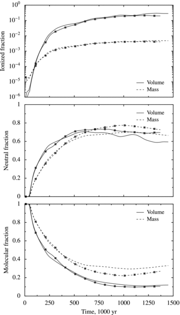
In Figs 11 and 12, we compare how the ionized, neutral and molecular gas component fractions vary throughout the evolution of the H ii regions. We calculate both volume and mass fractions for each component. The ionized gas in both the O- and B-star cases is thermally dominated, and there is no discernible distinction between the MHD and purely HD results. In the O-star case, the ionized fraction comes to occupy 90 per cent of the volume but only 10 per cent of the mass of the computational box by the end of the simulation. In the B-star case, the H ii region does not manage to globally break out of the computational box and so even at the end of the simulation the volume occupied by ionized gas is less than 30 per cent. The mass fraction is <1 per cent in this case, since the density in the ionized gas is low. The neutral gas is most affected by the magnetic field for both O- and B-star simulations. Figs 11 and 12 show that the MHD simulation has both higher mass and higher volume fractions of neutral gas than the purely HD results. The neutral component is more important in the B-star case than in the O-star case, reaching ∼70 per cent of the mass and volume fractions after 500 000 yr and remaining roughly constant thereafter. In the O-star case, however, the mass fraction remains roughly constant for the second half of the simulation while the volume fraction decreases sharply. This difference in behaviour can be attributed to the greater fragmentation in the O-star case (both MHD and HD) compared to the B star. The neutral material in the B-star simulation is distributed in a quite broad, smooth, almost uniform density region around the H ii region, whereas in the O-star simulation the neutral region around the photoionized gas is relatively thin but there is also neutral material inside the dense clumps and filaments that are formed by radiation-driven implosion, which have high density but low volume.

Figure 11

Ionized, neutral and molecular gas fractions by volume (solid lines) and mass (dashed lines) for the evolving H ii region around the O star. Lines with symbols are for the MHD simulation, while lines without symbols are for the purely HD case.

Open in new tabDownload slide

Figure 12

Same as Fig. 11 but for the B star.

Open in new tabDownload slide

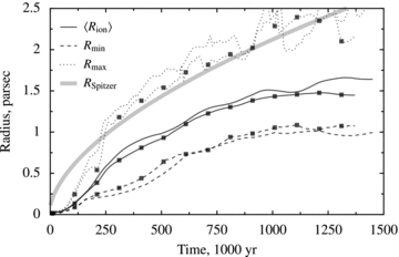
The expansion of an H ii region in a clumpy medium is not so easy to characterize. In Figs 13 and 14 we plot a variety of different measures of the radius of the photoionized region as functions of time, together with the analytical solution obtained using equation (1) for a medium of uniform density n₀ = 10³ cm⁻³. We calculate the mean radius² and also the minimum and maximum radii of the ionization front. For the H ii region around the O star, the mean radius closely follows the analytical solution for a long period of the simulation, possibly because the filling factor of the dense clumps and filaments which retard the ionization front is small. The maximum radius for the ionization front for the O-star simulation quickly becomes equal to the distance to the edge of the computational box and therefore has no physical meaning after this point. Until it leaves the box, the maximum radius represents the direction in which the ionization front is able to expand most quickly, i.e. a path of lowest density radially outwards from the star.

Figure 13

Expansion of the H ii region with time for the O star. The thick grey line represents the analytical solution. Also shown are the mean radius (solid lines), the maximum radius (dotted lines) and the minimum radius (dashed lines) of the ionization front. Lines with symbols are for the MHD simulation, while lines without symbols are for the purely HD case.

Open in new tabDownload slide

Figure 14

Same as Fig. 13 but for the B star.

Open in new tabDownload slide

For the B-star simulation, the mean radius is always below the analytical solution. Since this is true for both the MHD and purely HD simulations, it cannot be due to the magnetic field. The reason is that for the B star, the initial clump in which the star is embedded has a greater effect on the subsequent evolution of the H ii region than in the O-star case. In fact, we see that the maximum radius of the ionization front in the B-star H ii region does follow the analytical solution. The maximum radius follows the expansion of the ionization front in the direction where it was first able to break out of the dense clump in which the star was embedded. We have already seen that the neutral medium around the H ii region in the B-star case takes on a smooth and homogeneous appearance and that the mean molecular and neutral gas densities are roughly constant in time. Once the ionization front has managed to break out of the clump, therefore it follows the expansion law for a uniform medium in this mean density. In the majority of directions, however, the ionization front takes much longer to break out of the initial clump and so the mean ionization front radius is retarded compared to the analytical solution.

In both O- and B-star simulations, the minimum radius of the ionization front indicates the presence of fingers and clumps of neutral material within the H ii region. For the O-star simulation we have already mentioned how the magnetic field suppresses fragmentation, and this is reflected in the graph of minimum radius with time: fingers and globules formed in the purely HD simulation are denser and survive longer closer to the star compared to the MHD simulation. In the B-star case there is much less fragmentation and we see no fingers and clumps of neutral gas within the H ii region, and the minimum radii of both MHD and HD simulations seen in Fig. 14 bear this out.

In Figs 15 and 16, we show the mean radial velocities for the three gas components. Again, we compare the results of both MHD (lines with symbols) and purely HD simulations. Beginning with the ionized gas component, we see that for the O star the rms velocities reach a peak of about 8 km s⁻¹ and then decrease very slowly, which is what we saw in our previous paper (Mellema et al. 2006a). The mean radial velocity, on the other hand, peaks at 8–10 km s⁻¹ and then declines quite quickly. The rms velocities are due to interacting photoevaporated flows within the H ii region, which lead to gas flowing inwards as well as outwards (Henney 2003). The mean radial velocity traces the general expansion of the photoionized gas. We see that for the non-uniform medium, the initial expansive motions are more rapid than for the simple analytical model but this is just because the gas first begins to expand into regions of lowest density (Shu et al. 2002). There is a small difference between the rms velocities in the MHD and HD cases, with the latter being marginally higher. This could be due to the greater degree of fragmentation in the HD simulations which, in turn, leads to stronger photoevaporated flows.

Figure 15

Mean gas radial velocities within the ionized, neutral and molecular gas components for the O-star simulation. The thick grey line represents the analytical mean radial velocity. Also shown are the rms radial velocities (solid lines) and the mean radial velocity (dashed lines) of the gas. Lines with symbols are for the MHD simulation, while lines without symbols are for the purely HD case.

Open in new tabDownload slide

Figure 16

Same as Fig. 15 but for the B star.

Open in new tabDownload slide

In the B-star simulation the rms velocities are similar to the O-star case just discussed, which suggests that photoevaporated flows are important in this H ii region, too. The pure HD simulation shows slightly higher velocities than the MHD case, which indicates that the magnetic field plays some role in reducing the importance of photoevaporated flows within the ionized gas. The mean radial velocities show the same sort of ringing seen in the test problem of H ii region expansion in a uniform density medium (see Fig. 2). The period of the oscillations is of the order of 2 × 10⁵ yr, which is consistent with the sound-crossing time of the photoionized region. Note that in both O- and B-star simulations, the actual mean radial velocities are considerably higher than the corresponding analytical values for expansion in a uniform medium with density equal to the mean density of the initial computational box (n₀ = 1000 cm⁻³).

The neutral gas velocities show more separation between HD and MHD results, with the HD velocities being consistently higher in both mean and rms velocities. Interestingly, the different simulation velocities appear to depart from each other at a specific point in time, which is different depending on whether the mean or rms velocity is considered. This is true for both O- and B-star simulations. In the O-star case, after the initial acceleration, the neutral gas velocities reach 4–5 km s⁻¹, while for the B star the velocities are 1–2 km s⁻¹ lower and show evidence for ringing as for the ionized gas.

The initial molecular gas velocities reflect the Mach 10 supersonic turbulence of the underlying density distribution. At early times, there is evidence of residual infalling motions, i.e. negative radial velocities, again from the initial conditions. These persist longer in the B-star simulations than in the O-star simulations. This is because the O star rapidly ionizes out to the edge of the computational box, and the molecular material which remains is being accelerated radially away from the central star in clumps that are experiencing the rocket effect. In the B-star case, most of the molecular material surrounding the H ii region remains undisturbed, and so the imprint of the initial conditions remains in this gas until the end of the simulation.

In summary, we find slight differences in the expansion of H ii regions between MHD and purely HD simulations but the greatest differences are due to the different ionizing and FUV fluxes of the central O or B star. Most of the differences between the MHD and HD cases are due to the lesser amount of fragmentation in the former, indicating that magnetic fields provide some support to the neutral gas against radiation-driven implosions.

3.3 Magnetic quantities

Even though we find that the presence of a magnetic field only has small effects on the growth of the H ii region, this does not mean that the field is uninteresting or unimportant. For one thing, the field is important in the still neutral medium, where it constitutes a significant fraction of the total energy.

In Fig. 17, we show the magnetic field and the distribution of the photoionized gas for the B-star case in the same format as Figs 3 and 4. We can see that the magnetic field looks very different. The initial conditions were the result of an MHD turbulence calculation and in the molecular gas (coloured grey/white in the bottom panels of Fig. 17) we can see that the field appears to be randomly oriented.

Figure 17

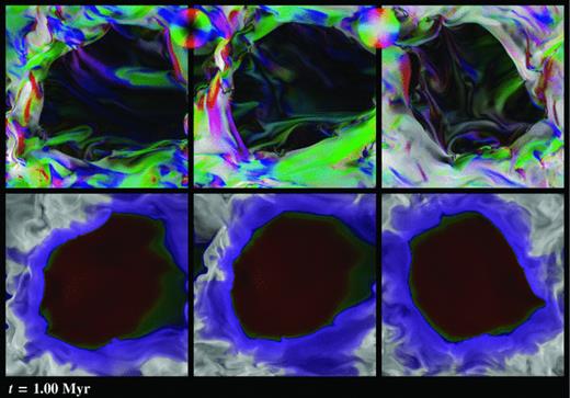
Magnetic field and photoionized gas distribution in the central x–y (left), x–z (centre) and y–z planes for the B-star simulation after 10⁶ yr. Colours have the same meaning as in Fig. 3.

Open in new tabDownload slide

In the warm, neutral (PDR) gas (coloured purple in the lower panels of the figure) there is strong evidence that the magnetic field is being aligned parallel to the ionization front, particularly in the bottom-left region of the x–y and x–z plots. At some points in this image, the ionization front has left the grid, and the periodic boundary condition in this simulation means that ionized material exits one side of the grid and reappears at the opposite boundary, where it will usually recombine because of the high column density through the molecular and neutral gas to the star at this position. At this point in the simulation, this is not affecting the global evolution of the H ii region and the surrounding warm, neutral gas.

The photoionized region has a very low magnetic field intensity, showing that the field has been pushed aside by the expansion of the H ii region. Photoevaporated flows from density inhomogeneities in both the neutral and molecular gas drag the magnetic field with them into the photoionized region in long filamentary structures. However, there is little mass associated with these flows. In the x–y and x–z central planes, there is a large region of partially ionized gas. This is also in the direction where the ionization front has left the grid and could be due to a density or velocity gradient, which results in the ionization front being unable to keep up with the gas, since it is no longer preceded by a neutral shock in this part of the computational grid.

In order to analyse the role of the magnetic field in our three components, ionized, neutral and molecular, we present colour plots showing the joint distribution of various quantities in these three components. Since the B- and O-star results are quite comparable, we only show the B-star results.

We start by considering the joint distribution of the magnetic field strength against the density. Fig. 18 shows this for the case of the B star at t = 10⁶ yr. The distribution of the ionized material is shown in blue and displays a wide range of field strengths (0.1–10 μG) across a narrow range of densities (10–20 cm⁻³; in the case of the O star, these values are some five times higher). The diagonal lines show the Alfvén speeds. If the sound speed in the gas is smaller than v_A, the flow will be magnetically dominated. As can be seen, the ionized material does not reach Alfvén speeds of 10 km s⁻¹, the typical sound speed in the ionized medium. Consequently the ionized flow is never magnetically dominated, consistent with the results found in the previous sections.

Figure 18

Magnitude of B field (G) against number density (cm⁻³) for volume-weighted joint distributions in the case of the B star at t = 10⁶ yr. The diagonal lines correspond to constant Alfvén speeds of 10 and 1 km s⁻¹. The three colours represent ionized (blue), neutral (green) and molecular (red) material.

Open in new tabDownload slide

Another way to represent the role of the magnetic field is to plot the joint distribution of magnetic and ram (turbulent) pressure, as is done in Fig. 19. In full equipartition, the turbulent, magnetic and thermal pressures should all be equal. Since the H ii region is expanding through its thermal pressure, it is the thermal pressure which is the overall dominating one. Fig. 19 shows that of the other two pressure components, turbulent pressure mostly dominates over magnetic pressure. In only a few places in the H ii region, the magnetic pressure dominates.

Figure 19

Magnetic pressure versus turbulent pressure for volume-weighted joint distributions in the case of the B star at t = 10⁶ yr. Note that the scales are the same on both x- and y-axes. The diagonal line shows equal pressures. The three colours represent ionized (blue), neutral (green) and molecular (red) material.

Open in new tabDownload slide

In the neutral and molecular material (represented by green and red in the joint distribution figures), the situation is different. The joint distribution of density and magnetic field strength, Fig. 18, shows a wide range of densities (10²–10⁴ cm⁻³) and a narrower range of magnetic field strengths (mostly around 10–30 μG, although some areas, principally neutral ones, have magnetic fields as weak as 1 μG). The molecular material generally has higher densities than the neutral material. Since the sound speed in the neutral and molecular regions is 1 km s⁻¹ or less, they are mostly magnetically rather than thermally dominated. In the distribution of pressures, Fig. 19, one sees that the neutral and molecular material clusters around the equipartition of the magnetic and turbulent pressures. The molecular material has regions where the turbulent pressure dominates and others where the magnetic pressure dominates. The neutral (PDR) material has generally somewhat lower pressures and is closer to equipartition.

Fig. 18 can be compared to observationally derived values for the magnetic field and densities in H ii regions and their surroundings. Results of Harvey–Smith et al. (in preparation) on large Galactic H ii regions show ranges in magnetic field strengths and typical densities for the ionized, neutral and molecular components which are very comparable to what we find in our simulation results.

4 DISCUSSION

4.1 Comparison with observations: RCW 120

The H ii region RCW 120 and its surrounding medium have recently been extensively studied at near- to far-infrared wavelengths in the context of triggered star formation (Zavagno et al. 2007; Deharveng et al. 2009; Anderson et al. 2010; Martins et al. 2010; Zavagno et al. 2010). This small (3.5 pc diameter at 1.35 kpc distance; Zavagno et al. 2007) H ii region appears to have a single ionizing source, identified from Very Large Telescope SINFONI near-infrared spectroscopy and spectral line fitting to stellar atmosphere models as an O6–O8V/III star (Martins et al. 2010) with an effective temperature of T_eff = 37.5 ± 2 kK and ionizing photon rate of log Q_H = 48.58 ± 0.22. These observationally derived parameters are remarkably similar to those we have adopted for our O-star simulations and so an opportunity for a direct comparison of RCW 120 with our results presents itself.

Morphologically, the observations and simulation look very similar. In particular, Fig. 7, corresponding to the O-star simulation after 200 000 yr of evolution is the same size as the observed bubble RCW 120. The top panels of the figure show the optical emission (with extinction from dust), while the bottom panels show synthetic 6-cm radio free–free emission from the ionized gas (blue), generic PAH emission from the PDR (green) and cold molecular gas column density (red). Figs 1 and 2 of Deharveng et al. (2009) show the Hα emission from the ionized gas, the 8 - μm emission from PAHs in the PDR, m emission from warm dust in the photoionized region and m cold dust emission from the neutral and molecular gas. If the reader mentally rotates the simulated images so that the bottom-left corner moves to the top centre, then a certain correspondence between simulations and observations can be imagined. The ionized gas emission fills the central cavity. In the optical, the images appear criss-crossed by dust lanes. Some of these are foreground; others are the result of projection of filaments and ridges deeper inside the H ii region. The PAH emission comes from a thin shell around the periphery of the H ii region, with projection seeming to put some PAH emission in the interior of the H ii region, as can be seen in both the simulation and the observations. The simulated PAH emission presents the same sort of irregularities, filaments and clumps as are seen in the observations.

The initial total mass in the computational box is ∼2000 M_⊙. After 200 000 yr of evolution, the mass distribution, as seen in Fig. 11, is approximately 5 per cent ionized gas, 55 per cent neutral gas and 40 per cent molecular gas. Some of the molecular gas is undisturbed material at the edge of the computational box but quite a large proportion must be in the clumps and filaments in the H ii region and PDR, where it becomes compressed by radiation-driven implosion. The H ii region has influenced virtually all of the computational domain by this time, and the ∼2000 M_⊙ of neutral and molecular material is comparable to the 1100–2100 M_⊙ derived by Zavagno et al. (2007) and Deharveng et al. (2009) from the m cold dust emission. This dust will be present in both the neutral and the molecular gas. Hence, we can surmise that the average density in the vicinity of RCW 120 is similar to that in our computational box, that is 〈n₀〉 = 10³ cm⁻³, though, of course, the density distribution is far from homogeneous. From this, we could go so far as to postulate that the age of RCW 120 must be similar to the time depicted in our simulation, that is, of the order of 200 000 yr. Martins et al. (2010) were unable to assign an age to RCW 120 except to say that it must be younger than 5 Myr.

Although radiation-driven implosion does enhance the density of photoionized globules at the periphery of the simulated H ii region, the fact that we do not include self-gravity in our simulations means that we are unable to model triggered star formation in the neutral shell around the H ii region. However, it is quite likely that radiation-driven implosion could trigger gravitational collapse in clumps that are already on the point of forming stars.

There are other potentially important physical processes that we do not include in our models. Dust grains are an important component of the interstellar medium in star-forming regions. They absorb ionizing photons, and both observations (e.g. Wood & Churchwell 1989) and theory (e.g. Arthur et al. 2004) suggest that more than 50 per cent of all the ionizing photons are absorbed by dust within the H ii regions in the initial stages of evolution when the ionized density is high. Radiation pressure on dust grains can form a central cavity in the H ii region (Mathews 1967; Inoue 2002), which can be as large as 30 per cent of the ionization front radius. Such cavities have been known for a long time from the optical observations of H ii regions (e.g. Menon 1962) and are also seen in more recent infrared observations (e.g. Watson et al. 2008). Krumholz & Matzner (2009) have studied the effect of radiation pressure on the dynamics of H ii regions and conclude that it is only an important effect for massive star clusters and not for H ii regions around individual massive stars. Stellar winds are also to be expected from stars whose effective temperatures are greater than 25 000 K, and these winds will provide an alternative mechanism for evacuating a central cavity in the dust and gas distribution in the H ii region. The mechanical luminosity of the stellar wind is converted into thermal pressure by shock waves (Dyson & Williams 1997), and this could affect the dynamics of the H ii region.

4.2 Predicted maps of the projected magnetic field

Figs 20–23 show visualizations of the projected integrated B field (line-of-sight and plane-of-sky components) from our simulations. These visualizations represent generic idealized versions of maps that can be obtained from various observational techniques. The line-of-sight field component can be determined from the Faraday rotation measure (Heiles et al. 1981) for ionized gas or from Zeeman spectroscopy (Brogan & Troland 2001) for neutral/molecular gas. The plane-of-sky field components can be determined from the observations of polarized emission or absorption (Kusakabe et al. 2008) from aligned spinning dust grains. In all of these techniques, the determination of B is not straightforward and relies on many auxiliary assumptions. In particular, it is very difficult to determine the absolute magnitude of the plane-of-sky field components except via statistical techniques such as the Chandrasekhar–Fermi method (Chandrasekhar & Fermi 1953; Heitsch et al. 2001; Ostriker, Stone & Gammie 2001; Falceta-Gonçalves, Lazarian & Kowal 2008). Furthermore, many of the techniques do not uniformly sample all regions along the line of sight, but are biased towards regions with particular physical conditions. We therefore caution against direct comparison of observational results with our maps in any but a qualitative sense. The maps are none the less useful in showing an overview of the magnetic field geometry in our simulations. In the following discussion, we describe locations on the projected map using the points of the compass, assuming that north is up (positive y) and east is left (negative x).

Figure 20

Projected magnetic field of the O-star model at a time of t = 200 000 yr, showing the full simulation cube (extent of 4 pc along each axis). The horizontal and vertical graph axes correspond to the simulation of x- and y-axes, respectively. The three grey-scale images (top-left, top-right and bottom-right panels) show the line-of-sight integral of the line-of-sight component of the magnetic field, weighted by the ionized (top-left), neutral (top-right) or molecular (bottom-right) gas density. The superimposed red vectors indicate the magnitude and direction of the line-of-sight integral of the plane-of-sky components of the magnetic field, using the same weightings. The integrals of the plane-of-sky components were carried out in a Stokes QU frame, as described in Appendix A. Blue contour lines show the column density of molecular gas, to aid comparison between the panels. The bottom-left panel shows a composite image of the column densities of molecular (red), neutral (green) and ionized (blue) gas. The normalization varies between the panels. For the column densities (bottom-left panel and contours), the maximum plotted values in units of H nuclei per cm² are 3.7 × 10²¹ (ionized), 5.1 × 10²² (neutral) and 1.3 × 10²³ (molecular). For the projected magnetic fields, the maximum plotted values in units of μG times H nuclei per cm² are 5.2 × 10²² (ionized, top left), 2.1 × 10²⁴ (neutral, top right) and 1.7 × 10²⁴ (molecular, bottom right).

Open in new tabDownload slide

Figure 21

Projected magnetic field of the B-star model at a time of t = 10⁶ yr, showing the full simulation cube (extent of 4 pc along each axis). Panels are the same as in Fig. 20. For the column densities (bottom-left panel and contours), the maximum plotted values in units of H nuclei per cm² are 2.1 × 10²⁰ (ionized), 4.6 × 10²² (neutral) and 3.4 × 10²² (molecular). For the projected magnetic fields, the maximum plotted values in units of μG times H nuclei per cm² are 1.0 × 10²¹ (ionized, top left), 7.5 × 10²³ (neutral, top right) and 7.2 × 10²³ (molecular, bottom right).

Open in new tabDownload slide

Figure 22

Projected magnetic field of the O-star model at a time of t = 200 000 yr, showing a 4 × zoom centred on the southern dense globule (extent of 1 pc along each axis). Panels are the same as in Fig. 20. For the column densities (bottom-left panel and contours), the maximum plotted values in units of H nuclei per cm² are 3.7 × 10²¹ (ionized), 2.7 × 10²² (neutral) and 1.3 × 10²³ (molecular). For the projected magnetic fields, the maximum plotted values in units of μG times H nuclei per cm² are 2.6 × 10²² (ionized, top left), 1.0 × 10²⁴ (neutral, top right) and 2.2 × 10²⁴ (molecular, bottom right).

Open in new tabDownload slide

Figure 23

Projected magnetic field of the B-star model at a time of t = 10⁶ yr, showing a 4 × zoom centred on the southern dense globule (extent of 1 pc along each axis). Panels are the same as in Fig. 20. For the column densities (bottom-left panel and contours), the maximum plotted values in units of H nuclei per cm² are 1.7 × 10²⁰ (ionized), 1.5 × 10²² (neutral) and 3.2 × 10²² (molecular). For the projected magnetic fields, the maximum plotted values in units of μG times H nuclei per cm² are 5.1 × 10²⁰ (ionized, top left), 3.8 × 10²³ (neutral, top right) and 3.6 × 10²³ (molecular, bottom right).

Open in new tabDownload slide

The most striking aspect of Figs 20 and 21 is the large-scale order that is apparent in the projected magnetic field. This is particularly visible in the neutral-weighted maps (top-right panels), where it can be seen that the field is frequently oriented parallel to the large-scale ionization front, forming a ring around the H ii region. The effect is particularly strong along the north and south borders of the region because of the net positive field along the x-axis (see Section 3.1), but it is also seen to a lesser extent along the east and west borders, despite the fact that the mean y-component of the field is zero. This is because of the fast-mode MHD shock that is driven into the surrounding gas by the expanding H ii region and which compresses both the gas and the field, tending to bend the field lines so that they are more closely parallel to the shock than they were in the undisturbed medium. A large-scale pattern is much harder to discern in the molecular-weighted maps (bottom-right panels), partly because the molecular column density is much less smoothly distributed, being concentrated in globules and filaments.

In most dense filaments, the field direction is parallel to the long axis of the filament, as can be seen particularly clearly in Fig. 22, which shows a detailed view of the dense photoevaporating globule found to the south in Fig. 20 and which is fed by multiple neutral/molecular filaments. In the molecular gas at the head of the globule, the magnetic field is bent into a hairpin shape. The B field in the ionized gas at the head of the globule tends to be oriented perpendicular to the ionization front, as is the case with almost all the dense globules visible in Fig. 20. The same is true along much of the bar-like feature to the west of the globule. On the other hand, in a few regions, such as along the filament that extends south from the globule, the B field in the ionized gas lies along the ionization front.

Fig. 23 shows a detailed view of the same dense southern globule, but from the B-star simulation shown in Fig. 21. The molecular gas shows a similar field pattern to that seen in the O-star case: the field goes up one of the feeding filaments and down the other, with a hairpin bend in between. Although this can be seen clearly in the molecular gas, the neutral and ionized gas show very different patterns, with magnetic field vectors that are generally perpendicular to the filament and continuous with the large-scale field pattern in the region. This is because the total ionized and neutral columns are dominated by diffuse material along the line of sight, rather than by material associated with the globule and filament.

4.3 Effects of the magnetic field on globule formation and evolution

It is interesting to compare the properties of the globules generated in our turbulent simulations with the results of previous detailed studies of the photoionization of isolated dense globules (Williams 2007; Henney et al. 2009; Mackey & Lim 2011). The principal findings of the earlier studies are that a sufficiently strong magnetic field (β < 0.01 in the initial neutral globule) will produce important qualitative changes in the photoevaporation process. Depending on the initial field orientation with respect to the direction of the ionizing photons, either extreme flattening of the globule may occur (perpendicular orientations) or the radiative implosion of the globule may be prevented (parallel orientations). For all orientations, the ionized photoevaporation flow cannot freely escape from the globule, leading to recombination at late times. On the other hand, a weaker field (β≃ 0.01 in the initial globule) leads only to a moderate flattening of the globule and does not prevent the free escape of the ionized photoevaporation flow.

In our turbulent simulations, the mean initial value of β is ≃0.032 (Section 3.1), which is intermediate between the two cases discussed above and might lead one to suspect that magnetic effects on the evolution of globules should be substantial. However, this is not the case. A careful examination of the three-dimensional globule morphologies in our simulations shows no evidence of magnetically induced flattening. Although many globules do show asymmetries, this is true equally of our non-magnetic simulations and is presumably due to their irregular initial shape and internal turbulent motions. The only difference in the globule properties between our non-magnetic and magnetic simulations is that the very smallest globules do not seem to form in the magnetic case.

In order to explain this apparent discrepancy with earlier work, it is necessary to examine in more detail the distribution of the magnetic field in the initial conditions of our turbulent simulations. It turns out that the dense filaments of molecular gas (from which the globules will ultimately form) tend to be much less magnetically dominated than the more diffuse gas, typically showing β > 0.1. Furthermore, these filaments already show a magnetic geometry similar to that described above (Section 4.2), with the field running along the long axis of the filament and with the field changing sign as one moves across the short axis. This is very different from the initial conditions assumed in the earlier globule photoevaporation studies, which were a uniform magnetic field that threaded a spherical globule (e.g. fig. 1 of Henney et al. 2009). As a result, the compressed globule heads in our turbulent simulations show approximately equal thermal and magnetic pressures (β∼ 1) and the magnetic effects are very modest. One caveat to this result is that numerical diffusion due to our limited spatial resolution may be producing non-physical magnetic reconnection in the globule head when oppositely directed field lines are forced together. Higher resolution studies of globule implosion with realistic initial field configurations are required in order to clarify this and these should also include self-gravity, which may be important during the phase of maximum compression (Esquivel & Raga 2007).

5 CONCLUSIONS

We have performed radiation-MHD simulations of the formation and expansion of H ii regions and PDRs around an O star and a B star in a turbulent magnetized molecular cloud on scales of up to 4 pc. Our principal conclusions are as follows.

• The expansion of the H ii region is little affected by the presence of the magnetic field, since the thermal pressure of the ionized gas dominates the dynamics on the time-scales of our simulations (Section 3.2.2).

• The O-star simulations produce greater fragmentation and denser clumps and filaments around the periphery of the H ii region than the B-star case (Section 3.2.1, Figs 7 and 8).

• For B stars, the non-ionizing FUV radiation plays an important role in determining the morphology of the region. H ii regions around such stars are surrounded by a thick, relatively smooth shell of neutral material (PDR), ∼30 per cent of the bubble radius (e.g. bottom panels of Fig. 17). In the O-star simulations, the PDR is thinner and more irregular in shape (e.g. Fig. 7).

• The resemblance at optical and longer wavelengths of our simulations to observed bubbles is striking (Section 4.1; Deharveng et al. 2009, 2010). Our ∼2-pc radius bubbles are a typical size compared to bubbles at known distances in the GLIMPSE surveys (Churchwell et al. 2006, 2007), and so comparisons are meaningful.

• The expanding H ii region and PDR tend to erase pre-existing small-scale disordered structure in the magnetic field, producing a large-scale ordered field in the neutral shell, with orientation approximately parallel to the ionization front (top panels of Fig. 17 and top-right panels of Figs 20 and 21).

• Dense evaporating globules, pillars and elephant trunk structures tend to be fed by two or more neutral/molecular filaments, with magnetic fields running along their length (right-hand panels of Fig. 22 and bottom-right panel of Fig. 23). The field geometry in the neutral and molecular gas at the bright head of the structure tends to be of a hairpin shape.

• The weak magnetic field in the ionized gas also shows an ordered structure. On the largest scales and at the latest times, it tends to align (albeit weakly in the O-star case), with the mean field direction of the simulation’s initial conditions (Fig. 21, top-left panel). On smaller scales, there is a general (but not universal) tendency for the field in ionized gas to be oriented perpendicular to the local ionization front. This tendency is more pronounced in the O-star simulation (Fig. 20, top-left panel) and in globule evaporation flows for both simulations (top-left panels of Figs 22 and 23).

• The highest pressure-compressed neutral/molecular gas shows approximate equipartition between thermal, turbulent and magnetic energy density, whereas lower pressure gas (either neutral or molecular) tends to separate into, on the one hand, magnetically dominated, quiescent regions, and, on the other hand, demagnetized, highly turbulent regions (Section 3.3, Fig. 19).

  The lower pressure gas also separates into low-β, magnetically dominated regions (which are largely molecular) and high-β, thermally dominated regions (which are largely neutral). The ionized gas, on the other hand, always shows approximate equipartition between thermal and turbulent energies, but with the magnetic energy being lower by 1–3 orders of magnitude.

• Velocity dispersions in the ionized gas of 7–9 km s⁻¹ are maintained for the entire duration of all our simulations (Section 3.2.2, Figs 15 and 16). This is five to 10 times higher than the value that would be predicted by expansion in a uniform medium. At early times (t < 100 000 yr for the O star or t < 300 000 yr for the B star), this dispersion is mainly due to radial champagne-flow expansion as the H ii region escapes from its natal clump. At later times, the net radial expansion of ionized gas subsides, but the velocity dispersion is maintained by inwardly directed photoevaporation flows from globules and pillars.

SJA and WJH acknowledge financial support from DGAPA PAPIIT projects IN112006, IN100309 and IN110108. This work was supported in part by Swedish Research Council grant 2009-4088. Some of the numerical calculations in this paper were performed on the Kan Balam supercomputer maintained and operated by DGSCA, UNAM. This work has made extensive use of NASA’s Astrophysics Abstract Data Service and the astro-ph archive.

REFERENCES

Appendix

APPENDIX A: INTEGRATION OF PLANE-OF-SKY FIELD COMPONENTS

Polarization-based methods for measuring the plane-of-sky components of the magnetic field cannot distinguish the sense of the field and are degenerate between position angles θ and θ+ 180°. It is therefore not sufficient to simply integrate B_x and B_y along the line of sight with appropriate weighting; neither is it sufficient to integrate B²_x and B²_y, since this will always give a result in the first quadrant (B_x, B_y > 0). In order to calculate our projected magnetic field maps (Section 4.2), we therefore adopt a ‘Stokes parameter’ approach (Chandrasekhar 1960), whereby the plane-of-sky components B_x(x, y, z) and B_y(x, y, z) are first transformed to (Q, U) space as and ⁠, where and θ = tan ⁻¹(B_y/B_x). Then the line-of-sight integration is performed as ⁠, where n is the relevant density (ionized, neutral or molecular). Finally, the components of the projected field are transformed back to (x, y) space: ⁠, ⁠, where and θ = 0.5 tan ⁻¹(M_U/M_Q).