


Abstract
The Galaxy and Mass Assembly (GAMA) survey has been operating since 2008 February on the 3.9-m Anglo-Australian Telescope using the AAOmega fibre-fed spectrograph facility to acquire spectra with a resolution of R≈ 1300 for 120 862 Sloan Digital Sky Survey selected galaxies. The target catalogue constitutes three contiguous equatorial regions centred at 9h (G09), 12h (G12) and 14.5h (G15) each of 12 × 4 deg2 to limiting fluxes of rpet < 19.4, rpet < 19.8 and rpet < 19.4 mag, respectively (and additional limits at other wavelengths). Spectra and reliable redshifts have been acquired for over 98 per cent of the galaxies within these limits. Here we present the survey footprint, progression, data reduction, redshifting, re-redshifting, an assessment of data quality after 3 yr, additional image analysis products (including ugrizYJHK photometry, Sérsic profiles and photometric redshifts), observing mask and construction of our core survey catalogue (GamaCore). From this we create three science-ready catalogues: GamaCoreDR1 for public release, which includes data acquired during year 1 of operations within specified magnitude limits (2008 February to April); GamaCoreMainSurvey containing all data above our survey limits for use by the GAMA Team and collaborators; and GamaCoreAtlasSV containing year 1, 2 and 3 data matched to Herschel-ATLAS science demonstration data. These catalogues along with the associated spectra, stamps and profiles can be accessed via the GAMA website: http://www.gama-survey.org/
1 INTRODUCTION
Large-scale surveys are now a familiar part of the astronomy landscape and assist in facilitating a wide range of science programmes. Three of the most-notable wide-area surveys in recent times, with a focus on galactic and galaxy evolution, are the Two-Micron All-Sky Survey (2MASS; Skrutskie et al. 2006), the Two-degree Field Galaxy Redshift Survey (2dFGRS; Colless et al. 2001, 2003) and the Sloan Digital Sky Survey (SDSS; York et al. 2000). Each of these surveys has been responsible for a wide range of science advances attested by their publication and citation records (Trimble & Ceja 2010): the identification of new stellar types (e.g. Kirkpatrick et al. 1999), tidal streams in the Galactic halo (e.g. Belokurov et al. 2006), new populations of dwarf galaxies (e.g. Willman et al. 2005), galaxy population statistics (e.g. Bell et al. 2003; Baldry et al. 2006), the recent cosmic star formation history (e.g. Heavens et al. 2004), group catalogues (e.g. Eke et al. 2004), merger rates (e.g. Bell et al. 2006), quantification of large-scale structure (e.g. Percival et al. 2001), galaxy clustering (e.g. Norberg et al. 2001) and, in conjunction with cosmic microwave background and Type Ia supernova searches, convergence towards the basic cosmological model now adopted as the standard (e.g. Spergel et al. 2003; Cole et al. 2005). In addition to these megasurveys, there have been a series of smaller, more specialized, local surveys including the Millennium Galaxy Catalogue (MGC; Driver et al. 2005), the 6dF Galaxy Survey (6dFGS; Jones et al. 2004, 2009), the H i Parkes All Sky Survey (Meyer et al. 2004) and the Galaxy Evolution Explorer (GALEX; Martin et al. 2005) mission, each of which is opening up new avenues of extragalactic exploration [i.e. structural properties, the near-infrared (near-IR) domain, the 21-cm domain and the ultraviolet (UV) domain, respectively]. Together these surveys provide an inhomogeneous nearby reference point for the very narrow high-z pencil beam surveys underway (i.e. DEEP2, VVDS, COSMOS, GEMS, etc.) from which comparative studies can be made to quantify the process of galaxy evolution (e.g. Cameron & Driver 2007).
The Galaxy and Mass Assembly (GAMA) survey has been established with two main sets of aims, which are described in Driver et al. (2009). The first is to use the galaxy distribution to conduct a series of tests of the cold dark matter (CDM) paradigm and the second is to carry out detailed studies of the internal structure and evolution of the galaxies themselves.
The CDM model is now the standard means by which data relevant to the galaxy formation and evolution are interpreted and it has met with great success on 10–100 Mpc scales. The next challenge in validating this standard model is to move beyond small linear fluctuations, into the regime dominated by dark matter haloes. The fragmentation of the dark matter into these roughly spherical virialized objects is robustly predicted both numerically and analytically over seven orders of magnitude in halo mass (e.g. Springel et al. 2005). Massive haloes are readily identified as rich clusters of galaxies, but it remains a challenge to probe further down the mass function. For this purpose, one needs to identify low-mass groups of galaxies, requiring a survey that probes far down the galaxy luminosity function over a large representative volume. But having found low-mass haloes, the galaxy population within each halo depends critically on the interaction between the baryon processes (i.e. star formation rate and feedback efficiency) and the total halo mass. In fact, the ratio of the stellar mass to halo mass is predicted (Bower et al. 2006; De Lucia et al. 2006) to be strongly dependent on the halo mass, exhibiting a characteristic dip at Local Group masses. The need for feedback mechanisms to suppress star formation in both low-mass haloes (via supernovae) and high-mass haloes [via active galactic nuclei (AGNs)] is now part of standard prescriptions in modelling galaxy formation. With GAMA we can connect these theoretical ingredients directly with observational measurements.
However, the astrophysics of the galaxy bias is not the only poorly understood area in the CDM model. Existing successes have been achieved at the price of introducing dark energy as the major constituent of the Universe and a key task for cosmology is to discriminate between various explanations for this phenomenon: a cosmological constant, time-varying scalar field or a deficiency in our gravity model. These aspects can be probed by GAMA in two distinct ways: either the form or evolution of the halo mass function may diverge from standard predictions of the gravitational collapse in the highly non-linear regime or information on non-standard models may be obtained from velocity fields on 10-Mpc scales. The latter induces redshift-space anisotropies in the clustering pattern, which measure the growth rate of the cosmic structure (e.g. Guzzo et al. 2008). Thus, GAMA has the potential to illuminate both the astrophysical and the fundamental aspects of the CDM model.
Moving beyond the large-scale distribution, GAMA’s main long-term legacy will be to create a uniform galaxy data base, which builds on earlier local surveys in a comprehensive manner to fainter flux levels, higher redshift, higher spatial resolution, and spanning UV to radio wavelengths. The need for a combined homogeneous, multiwavelength and spatially resolved study can be highlighted by three topical issues:
Galaxy Structure. Galaxies typically comprise bulge and/or disc components that exhibit distinct properties (dynamics, ages, metallicities, profiles, dust and gas content), indicating potentially distinct evolutionary paths (e.g. cold smooth and hot lumpy accretion; cf. Driver et al. 2006 or Cook et al. 2010). This is corroborated by the existence of the many supermassive black hole–bulge relations (see e.g. Novak, Faber & Dekel 2006), which firmly couples the spheroid-only evolution with the AGN history (Hopkins et al. 2006). A comprehensive insight into galaxy formation and evolution therefore demands consideration of the structural components requiring high spatial resolution imaging on ∼1 kpc scales or better (e.g. Allen et al. 2006; Gadotti 2009).
Dust attenuation. A recent spate of papers (Choi, Park & Vogeley 2007; Driver et al. 2007, 2008; Shao et al. 2007; Masters et al. 2010) have highlighted the severe impact of the dust attenuation on the measurement of basic galaxy properties (e.g. fluxes and sizes). In particular, the dust attenuation is highly dependent on the wavelength, inclination and galaxy type with the possibility of some further dependence on environment. Constructing detailed models for the attenuation of stellar light by dust in galaxies and subsequent re-emission (e.g. Popescu et al. 2000, 2011) is intractable without extensive wavelength coverage extending from the UV through to the far-IR. To survey the dust content for a significant sample of galaxies therefore demands a multiwavelength data set extending over a sufficiently large volume to span all environments and galaxy types. The GAMA regions are or will be surveyed by the broader GALEX Medium Imaging Survey and Herschel-ATLAS (H-ATLAS) (Eales et al. 2010) programmes, providing UV to far-IR coverage for a significant fraction of our survey area.
The Hicontent. As star formation is ultimately driven by a galaxy’s H i content, any model of galaxy formation and evolution must be consistent with the observed H i properties (see e.g. discussion in Hopkins, McClure-Griffiths & Gaensler 2008). Until recently probing H i beyond very low redshifts has been laborious, if not impossible, due to ground-based interference and/or sensitivity limitations (see e.g. Lah et al. 2009). The new generation of radio arrays and receivers are using radio-frequency interference mitigation methods coupled with new technology receivers to open up the H i Universe at all redshifts (i.e. ASKAP, MeerKAT, LOFAR and ultimately the SKA). This will enable coherent radio surveys that are well matched in terms of sensitivity and resolution to optical/near-IR data. Initial design study investment has been made in the DINGO project, which aims to conduct deep H i observations within a significant fraction of the GAMA regions using ASKAP (Johnston et al. 2007).
The GAMA survey will eventually provide a wide-area highly complete spectroscopic survey of over 400k galaxies with subarcsecond optical/near-IR imaging (SDSS/UKIDSS/VST/VISTA). Complementary multiwavelength photometry from the UV (GALEX), mid-IR (WISE), far-IR (Herschel) and radio wavelengths (ASKAP, GMRT) is being obtained by a number of independent public and private survey programmes. These additional data will ultimately be ingested into the GAMA data base as they become available to the GAMA Team. At the heart of the survey is the 3.9-m Anglo-Australian Telescope (AAT), which is being used to provide the vital distance information for all galaxies above well-specified flux, size and isophotal detection limits. In addition, the spectra from AAOmega for many of the samples will be of sufficiently high signal-to-noise ratio (S/N) and spectral resolution (≈3–6 Å) to allow for the extraction of line diagnostic information leading to constraints on star formation rates, velocity dispersions and other formation/evolutionary markers. The area and depth of GAMA compared to other notable surveys is detailed in Baldry et al. (2010; their fig. 1). In general, GAMA lies in the parameter space between that occupied by the very wide shallow surveys and the deep pencil beam surveys, and is optimized to study structure on ∼ to
to  scales, as well as sample the galaxy population from far-UV to radio wavelengths.
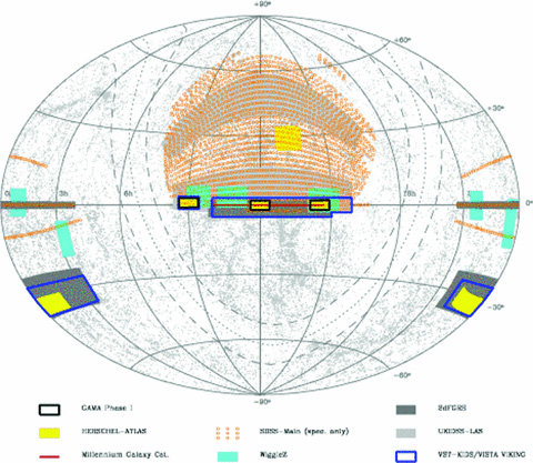
GAMA Phase I (black squares) in relation to other recent and planned surveys (see key). For a zoom-in to the GAMA regions showing the SDSS, UKIDSS and GALEX overlap, see fig. 1 of the companion paper describing the photometry by Hill et al. (2010a). Also overlaid as grey dots all known redshifts at z < 0.1 taken from the NED.
This paper describes the first 3 yr of the GAMA AAOmega spectroscopic campaign, which has resulted in 112k new redshifts (in addition to the 19k already known in these regions). In Section 2, we describe the spectroscopic progress, data reduction, redshifting, re-redshifting, an assessment of the redshift accuracy and blunder rate, and an update to our initial visual classifications. In Section 3, we describe additional image analysis resulting in ugrizYJHK-matched aperture photometry, Sérsic profiles and photometric redshifts. In Section 4, we describe the combination of the data presented in Sections 2 and 3 to form our core catalogue and investigate the completeness versus magnitude, colour, surface brightness, concentration and close pairs. In Section 5, we present the survey masks required for spatial clustering studies and in Section 6, we present our publicly available science ready catalogue. These catalogues along with an MySQL tool and other data inspection tools are now available at http://www.gama-survey.org/ and we expect future releases of redshifts and other data products to occur on an approximately annual cycle.
Please note that all magnitudes used in this paper, unless otherwise specified, are r-band Petrosian (rpet) from the SDSS DR6, which have been extinction corrected and placed on to the true AB scale following the prescription described by the SDSS DR6 (Adelman-McCarthy et al. 2008).
2 THE GAMA AAT SPECTROSCOPIC SURVEY
2.1 GAMA field selection, input catalogue and tiling algorithm
The initial GAMA survey consists of three equatorial regions, each of 12 × 4 deg2 (see Table 1 and Fig. 1). The decision for this configuration was driven by three considerations: suitability for large-scale structure studies demanding contiguous regions of ∼50 deg2 to fully sample ∼100 co-moving  structures at z≈ 0.2; observability demanding a 56h RA baseline to fill a night’s worth of observations over several lunations; and overlap with existing and planned surveys, in particular the SDSS (York et al. 2000), UKIDSS LAS (Lawrence et al. 2007), VST KIDS, VISTA VIKING, H-ATLAS (Eales et al. 2010) and ASKAP DINGO. Fig. 1 shows the overlap of some of these surveys. Note the H-ATLAS South Galactic Pole survey region has changed since fig. 5 of Driver et al. (2009) due to additional spacecraft limitations introduced in-flight. The depth and area of the GAMA AAT spectroscopic survey were optimized following detailed simulations of the GAMA primary science goal of measuring the halo mass function. This resulted in an initial survey area of 144 deg2 to a depth of rpet < 19.4 mag in the 9h and 15h regions, and an increased depth of rpet < 19.8 mag in the 12h region (see Table 1). In addition, for year 2 and 3 observations, an additional K- and z-band selection was introduced such that the final main galaxy sample (Main Survey) can be defined (see Baldry et al. 2010) as follows:
Coordinates of the three GAMA equatorial fields.
| Field | RA (J2000) | Dec. (J2000) | Area | Depth |
| (°) | (°) | (deg2) | (mag) | |
| G09 | 129.0...141.0 | +3.0... − 1.0 | 12 × 4 | rpet < 19.4 |
| G12 | 174.0...186.0 | +2.0... − 2.0 | 12 × 4 | rpet < 19.8 |
| G15 | 211.5...223.5 | +2.0... − 2.0 | 12 × 4 | rpet < 19.4 |
| Field | RA (J2000) | Dec. (J2000) | Area | Depth |
| (°) | (°) | (deg2) | (mag) | |
| G09 | 129.0...141.0 | +3.0... − 1.0 | 12 × 4 | rpet < 19.4 |
| G12 | 174.0...186.0 | +2.0... − 2.0 | 12 × 4 | rpet < 19.8 |
| G15 | 211.5...223.5 | +2.0... − 2.0 | 12 × 4 | rpet < 19.4 |
G09: rpet < 19.4 OR (KKron < 17.6 AND rmodel < 20.5) OR (zmodel < 18.2 AND rmodel < 20.5) mag
G12: rpet < 19.8 OR (KKron < 17.6 AND rmodel < 20.5) OR (zmodel < 18.2 AND rmodel < 20.5) mag
G15: rpet < 19.4 OR (KKron < 17.6 AND rmodel < 20.5) OR (zmodel < 18.2 AND rmodel < 20.5) mag with all magnitudes expressed in AB. For the remainder of this paper, we mainly focus, for clarity, on the r-band-selected data and note that equivalent diagnostic plots to those shown later in this paper can easily be created for the z- and K-band selections.
2.2 Survey preparation
The input catalogue for the GAMA spectroscopic survey was constructed from the SDSS DR6 (Adelman-McCarthy et al. 2008) and our own reanalysis of the UKIDSS LAS DR4 (Lawrence et al. 2007) to assist in the star–galaxy separation; see Hill et al. (2010a) for details. The preparation of the input catalogue, including extensive visual checks and the revised star–galaxy separation algorithm, is described and assessed in detail by Baldry et al. (2010). The survey is being conducted using the AAT’s AAOmega spectrograph system (an upgrade of the original 2dF spectrographs: Lewis et al. 2002; Sharp et al. 2006).
In year 1, we implemented a uniform grid tiling algorithm (see Fig. 2, upper panels), which created a significant imprint of the tile positions on the spatial completeness distribution. Subsequently, for years 2 and 3, we implemented a heuristic ‘greedy’ tiling strategy, which was designed to maximize the spatial completeness across the survey regions within 0 14 smoothed regions. Full details of the GAMA science requirements and the tiling strategy devised to meet these are laid out by Robotham et al. (2010). The efficiency of this strategy is discussed further in Section 5. The final location of all tiles is shown in Fig. 2 and the locations of objects for which redshifts were not secured or not observed are shown in the lower panels of Fig. 3 as black dots or red crosses, respectively.
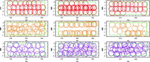
Location of the tiles in year 1 (top panels), year 2 (middle panels) and year 3 (bottom panels) for G09 (left-hand panels), G12 (middle panels) and G15 (right-hand panels).
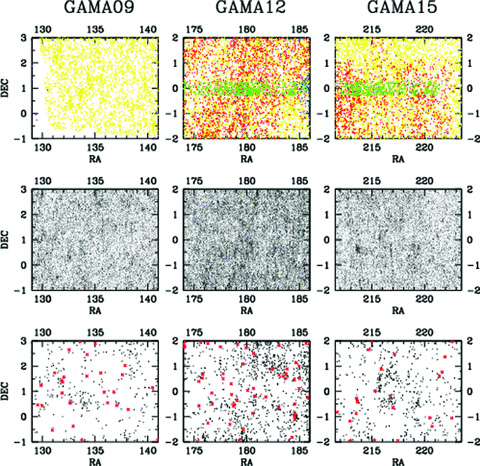
Top panel: the distribution of pre-existing redshifts (SDSS, yellow; 2dFGRS, red; MGC, green; other, blue) within the three regions (as indicated). Middle panel: the distributions of redshifts acquired during the GAMA Phase I campaign. Lower panel: the distribution of targets for which redshifts were not obtained (black dots) or were not targeted (red crosses).
2.3 Observations and data reduction
All GAMA 2dF pointings (tiles) were observed during dark or grey time with exposure times mostly ranging from 3000 to 5000 s (in three to five exposures) depending on seeing and sky brightness. Observations were generally conducted at an hour angle of less than 2 h (the median zenith distance of the observations is 35°) and with the Atmospheric Dispersion Corrector engaged. We used the 580V and 385R gratings with central wavelengths of 4800 and 7250 Å in the blue and red arms, respectively, separated by a 5700-Å dichroic. This set-up yielded a continuous wavelength coverage of 3720–8850 Å at a resolution of ≈3.5 Å (in the blue channel) and ≈5.5 Å (in the red channel). Every block of science exposures was accompanied by a flat-field and an arc-lamp exposure, while a master bias frame was constructed once per observing run. In each observation, fibres were allocated to between 318 and 366 galaxy targets (depending on the number of broken fibres), to at least 20 blank sky positions, to three to five SDSS spectroscopic standards and to six guide stars selected from the SDSS in the range 14.35 < rpet < 14.5 mag (verified via cross-matching with the USNO-B catalogue to ensure proper motions were below 15 mas yr−1). Galaxy targets were prioritized as indicated in Table 1 of Robotham et al. (2010). The locations of all 392 tile centres are shown in Fig. 2. The change in the tiling strategy from a fixed grid system in year 1 to the greedy tiling strategy in years 2 and 3 is evident from the latter leading to an extremely spatially uniform survey (see Section 5). The overall progress of the survey in terms of objects per night and the cumulative total numbers are shown in Fig. 4 illustrating that typically between 1500 and 2500 redshifts were obtained per night over the 3-yr campaign.
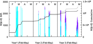
Progression of the GAMA survey in terms of spectra and redshift acquisition for years 1, 2 and 3 as indicated. The cyan line shows the number of spectra obtained per night within our Main Survey limits and the mauve shows the number below our flux limits (i.e. secondary targets and fillers). The solid line shows the cumulative distribution of redshifts within our survey limits and the dashed line shows the cumulative distribution of all redshifts. The cumulative distributions include pre-existing redshifts and are calculated monthly rather than nightly.
The data were reduced at the telescope in real time using the (former1) AAO’s 2dfdr software (Croom, Saunders & Heald 2004) developed continuously since the advent of the 2dF and recently optimized for AAOmega. The software is described in a number of AAO documents.2 Briefly, it performs automated spectral trace (tramline) detection, sky subtraction, wavelength calibration, stacking and splicing. As part of the automated 2dfdr reduction process, the blue and red spectra are flux calibrated to a white dwarf spectrum but with an arbitrary normalization. Future releases will include absolute flux-calibrated spectra. Following the standard data reduction, we attempted to improve the sky subtraction by applying a principal component analysis (PCA) technique similar to that described by Wild & Hewett (2005) and described in detail by Sharp & Parkinson (2010). We note that ∼5 per cent of all spectra are affected by fringing (caused by small air gaps between the adhesive that joins a fibre with its prism) and we are currently studying algorithms that might remove or at least mitigate this effect.
2.4 Redshifting
Each one of the fully reduced and PCA-sky-subtracted spectra were initially redshifted by one of the observers at the telescope using the code runz, which was originally developed by Will Sutherland for the 2dFGRS (now maintained by Scott Croom). runz attempts to determine a spectrum’s redshift (i) by cross-correlating it with a range of templates, including star-forming, E+A and quiescent galaxies, A, O and M stars, as well as QSO templates; and (ii) by fitting Gaussians to emission lines and searching for multiline matches. These estimates are quasi-independent because the strongest emission lines are clipped from the templates before the cross-correlation is performed. runz then proceeds by presenting its operator with a plot of the spectrum marking the positions of common nebular emission and stellar absorption lines at the best automatic redshift. This redshift is then checked visually by the operator who, if it is deemed incorrect, may use a number of methods to try to find the correct one. The process is concluded by the operator assigning a (subjective) quality (Q) to the finally chosen redshift:
Q = 4: The redshift is certainly correct. Q = 3: The redshift is probably correct. Q = 2: The redshift may be correct. Must be checked before being included in a scientific analysis. Q = 1: No redshift could be found. Q = 0: Complete data reduction failure.
With the above definitions, it is understood that by assigning Q≥ 3 a redshift is approved as suitable for inclusion in scientific analysis. Note that Q refers to the (subjective) quality of the redshift, not of the spectrum.
2.5 Re-redshifting
The outcome of the redshifting process described above will not be 100 per cent accurate. It is inevitable that some fraction of the Q≥ 3 redshifts will be incorrect. Furthermore, the quality assigned to a redshift is somewhat subjective and will depend on the experience of the redshifter. In an effort to weed out mistakes and to quantify the probability of a redshift being correct, thereby homogenizing the quality scale of our redshifts, a significant fraction of our sample has been independently re-redshifted. This process and its results will be described in detail by Liske et al. (in preparation). Briefly, the spectra of all Q = 2 and 3 redshifts, of all Q = 4 redshifts with discrepant photo-redshift, and of an additional random Q = 4 sample have been independently re-redshifted. In all, 25 individuals have been involved in the re-redshifting process which includes observers involved in the initial classification. Those conducting the re-redshifting had no knowledge of the originally assigned redshift or Q value. The Q = 2 sample was re-examined twice. Overall, approximately, one-third of the entire GAMA sample was re-evaluated. The results of the blind re-redshifting process were used to estimate the probability, for each redshifter, that she/he finds the correct redshift as a function of Q (for Q≥ 2) or that she/he has correctly assigned Q = 1. Given these probabilities, and given the set of redshift ‘opinions’ for a spectrum, we have calculated for each redshift found for this spectrum the probability, pz, that it is correct. This allowed us to select the ‘best’ redshift in cases where more than one redshift had been found for a given spectrum. It also allowed us to construct a ‘normalized’ quality scale: nQ = 4 if pz≥ 0.95 nQ = 3 if 0.9 ≤pz < 0.95 nQ = 2 if pz < 0.9 nQ = 1 if it is not possible to measure a redshift from this spectrum.
Unlike Q, whose precise, quantitative meaning depends on the redshifter who assigned it, the meaning of nQ is homogeneous across the entire redshift sample.
In Fig. 5, we show one example each of a spectrum with nQ = 4, 3 and 2.
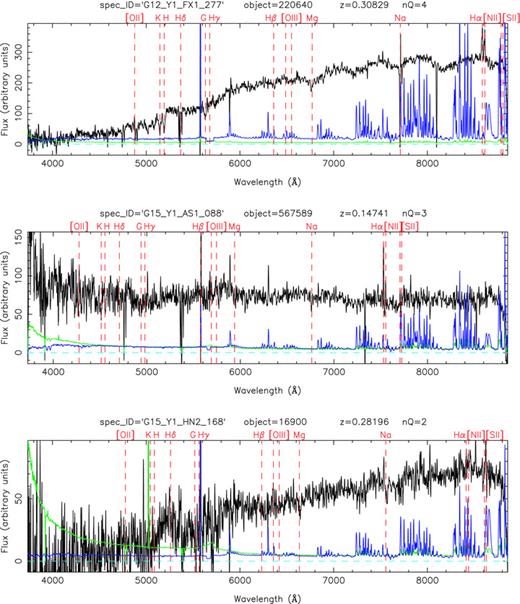
Examples of spectra with redshift quality nQ = 4 (top panel), 3 (middle panel) and 2 (bottom panel). We show the spectrum (black), the 1σ error (green) and the mean sky spectrum (blue, scaled arbitrarily with respect to the spectrum). The vertical dashed red lines mark the positions of common nebular emission and stellar absorption lines at the redshift of the galaxy. The spectra were smoothed with a boxcar of width 5 pixels. For more examples of GAMA spectra, see the data release website: http://www.gama-survey.org/database/
2.6 Final redshift sample
In the 3 yr of observation completed so far, we have observed 392 tiles, resulting in 135 902 spectra in total (including standard stars), and 134 390 spectra of 120 862 unique galaxy targets. Of these, 114 043 have a reliable redshift with nQ≥ 3, implying a mean overall redshift completeness of 94.4 per cent. Restricting the sample to the r-limited Main Survey targets (i.e. ignoring the K and z selection and fainter fillers), we find that the completeness is >98 per cent in all three GAMA regions, leaving little room for any severe spectroscopic bias. Fig. 6 shows the evolution of the survey completeness for the main r-band-limited sample versus apparent magnitude across (left-hand to right-hand side) the three GAMA regions.
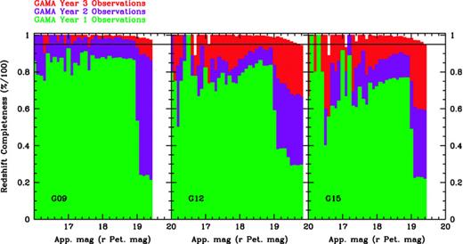
Evolution of the redshift completeness (Q≥ 3) of the GAMA survey (main r-band selection only) over 3 yr of observations showing the progressive build-up towards uniform high completeness. The horizontal line denotes a uniform 95 per cent completeness.
2.7 Redshift accuracy and reliability
Quantifying the redshift accuracy and blunder rate is crucial for most science applications and can be approached in a number of ways. Here we compare redshifts obtained for systems via repeat observations within GAMA (intra-GAMA comparison) and also repeat observations of objects surveyed by earlier studies (inter-survey comparison).
2.7.1 Intra-GAMA comparison
Our sample includes 974 objects that were observed more than once and for which we have more than one nQ≥ 3 redshift from independent spectra. The distribution of pairwise velocity differences, Δv, of this sample is shown as the shaded histogram in the left-hand panel of Fig. 7. This distribution is clearly not Gaussian but roughly Lorentzian (blue line), although with a narrower core, and there are a number of outliers (see below). Nevertheless, if we clip this distribution at ±500 km s−1, we find a 68-percentile range of 185 km s−1, indicating a redshift error σv = 65 km s−1. However, this value is likely to depend on nQ. Indeed, if we restrict the sample to pairs where both redshifts have nQ = 4 (red histogram), we find σv,4 = 60 km s−1. Our sample of pairs where both redshifts have nQ = 3 is small (22 pairs), but this yields σv,3 = 101 km s−1. However, given σv,4, we can also use our larger sample of pairs where one redshift has nQ = 3 and the other has nQ = 4 (green histogram) to obtain an independent estimate of σv,3 = 97 km s−1, which is in reasonable agreement.
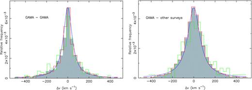
Left-hand panel: the shaded histogram shows the distribution of differences between the redshifts measured from independent GAMA spectra of the same objects, where all redshifts have nQ≥ 3 (868 pairs from 1718 unique spectra of 856 unique objects). The red histogram shows the same for pairs where both redshifts have nQ = 4 (617 pairs from 1216 unique spectra of 605 unique objects). The green histogram shows the same for pairs where one redshift has nQ = 3 and the other has nQ = 4 (229 pairs from 458 unique spectra of 229 unique objects). The blue line shows a Lorentzian with γ = 50 km s−1 for comparison. Right-hand panel: the shaded histogram shows the distribution of differences between the redshifts measured from independent GAMA and non-GAMA spectra of the same objects, where all redshifts have nQ≥ 3 (2533 pairs from 4892 unique spectra of 2359 unique objects). The red histogram shows the same for pairs where the GAMA redshift has nQ = 4 and the non-GAMA redshift has nQ≥ 3 (2385 pairs from 4618 unique spectra of 2233 unique objects). The green histogram shows the same for pairs where the GAMA redshift has nQ = 3 (148 pairs from 290 unique spectra of 142 unique objects). The blue line shows a Lorentzian with γ = 70 km s−1 for comparison.
Defining discrepant redshift pairs as those with |Δv| > 500 km s−1 and assuming that only one, but not both of the redshifts of such pairs, is wrong, we find that 3.6 per cent of redshifts with nQ = 4 are in fact wrong. This is in reasonable agreement with the fact that nQ = 4 redshifts are defined as those with pz > 0.95. However, for nQ = 3, we find a blunder rate of 15.1 per cent, which is somewhat higher than expected based on the fact that nQ = 3 is defined as pz > 0.9. We surmise that this is likely to be the result of a selection effect: many of the objects in this sample are likely to have been re-observed by GAMA, because the initial redshift of the first spectrum was only of a low quality (i.e. Q = 2). However, subsequent re-redshifting of the initial spectrum (after the re-observation) may have produced confirmation of the initial redshift, which will have bumped the redshift quality to nQ = 3. Hence, this sample is likely to include many spectra that are of worse quality and/or spectra that are harder to redshift than the average nQ = 3 spectrum, which will produce a higher blunder rate for this sample than the average blunder rate for the whole nQ = 3 sample. Indeed, the median S/N of this sample is 20 per cent lower than for the full GAMA sample. Note that this may also have an effect on the redshift accuracies determined above. This will be investigated in more detail by Liske et al. (in preparation).
2.7.2 Inter-survey comparisons
Our sample includes 2522 unique GAMA spectra (with nQ≥ 3 redshifts) for objects that had previously been observed by other surveys (see Section 2.8), for a total of 2671 GAMA–non-GAMA pairs. The distribution of the velocity differences of this sample is shown as the shaded histogram in the right-hand panel of Fig. 7. Approximately 81 per cent of the non-GAMA spectra in this sample are from the 2dFGRS and the MGC, which were both obtained with 2dF, using the same set-up and procedures. For the 2dFGRS, Colless et al. (2001) quote an average redshift uncertainty of 85 km s−1. Using this value together with the observed 68-percentile ranges of the velocity differences of the GAMA (nQ = 4, 3)–non-GAMA (nQ≥ 3) sample (red and green histograms, respectively) we find σv,4 = 51 km s−1 and σv,3 = 88 km s−1. These values are somewhat lower than those derived in the previous section. The most likely explanation for this is that the inter-survey sample considered here is brighter than the intra-GAMA sample of the previous section (because of the spectroscopic limits of the 2dFGRS and MGC). Indeed, the median S/N of the GAMA spectra in the inter-survey sample is a factor of 1.7 higher than that of the spectra in the intra-GAMA sample.
As above, we can also attempt to estimate the GAMA blunder rate from the inter-survey sample. From the GAMA (nQ = 4)–non-GAMA (nQ≥ 3) sample, we find a GAMA nQ = 4 blunder rate of 5.0 per cent if we assume that all redshift discrepancies are due to GAMA mistakes. However, this is clearly not the case since the blunder rate improves to 3.0 per cent if we restrict the sample to pairs with nQ≥ 4 non-GAMA redshifts. Similarly, the GAMA nQ = 3 blunder rate comes out at 10.1 or 4.2 per cent depending on whether one includes the pairs with non-GAMA nQ = 3 redshifts or not, considerably lower than the corresponding value derived in the previous section.
In summary, it seems likely that neither the intra-GAMA nor the inter-survey sample is fully representative of the complete GAMA sample. The former is on average of lower quality than the full sample, while the latter is of higher quality. Hence, we must conclude that the redshift accuracies and blunder rates determined from these samples are not representative either, but are expected to span the true values. A full analysis of these issues will be provided by Liske et al. (in preparation) following re-redshifting of the recently acquired year 3 data.
2.8 Merging GAMA with data from earlier redshift surveys
The GAMA survey builds upon regions of sky already sampled by a number of surveys, most notably the SDSS and 2dFGRS (as indicated in Table 2). As the GAMA input catalogue (Baldry et al. 2010) has taken the pre-existing redshifts into account, the GAMA data by themselves constitute a highly biased sample missing 80–90 per cent of bright sources with rpet < 17.77 mag and fainter objects previously selected by AGN or LRG surveys. It is therefore important for almost any scientific application, outside of analysing AAOmega performance, to produce extended catalogues that include both the GAMA and pre-GAMA data. Fig. 8 shows the n(z) distributions of redshifts in the three GAMA blocks to rpet < 19.4 mag in G09 and G15 and to rpet < 19.8 mag in G12 colour coded to acknowledge the survey from which they originate. Table 2 shows the contribution to the combined redshift catalogue from various surveys. Note the numbers shown in Table 2 may disagree with those shown in Baldry et al. (2010) as some repeat observations of previous targets were made.
Contribution from various surveys to the final GAMA data base.
| Survey | G09 | G12 | G15 | Reference or |
| source (Z_SOURCE) | r < 19.4 | r < 19.8 | r < 19.4 | acknowledgment |
| SDSS DR7 | 3190 | 4758 | 5092 | Abazajian et al. (2009) |
| 2dFGRS | 0 | 2107 | 1196 | Colless et al. (2001) |
| MGC | 0 | 612 | 497 | Driver et al. (2005) |
| 2SLAQ-LRG | 2 | 49 | 13 | Canon et al. (2006) |
| GAMAz | 26 783 | 42 210 | 25 858 | This paper |
| 6dFGS | 7 | 14 | 10 | Jones et al. (2009) |
| UZC | 3 | 2 | 1 | Falco et al. (1999) |
| 2QZ | 0 | 31 | 5 | Croom et al. (2004) |
| 2SLAQ-QSO | 1 | 1 | 1 | Croom et al. (2009) |
| NED | 0 | 2 | 3 | NED |
| z not known | 347 | 1145 | 591 | – |
| Total | 30 333 | 50 931 | 33 267 | – |
| Completeness (per cent) | 98.9 per cent | 97.8 per cent | 98.0 per cent |
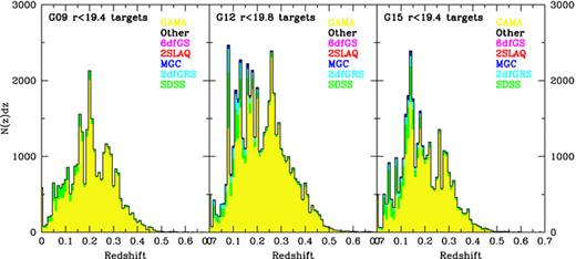
The n(z) distributions of the GAMA regions including new GAMA redshifts (shown in yellow) along side pre-existing redshifts already in the public domain as indicated.
2.9 Update to visual inspection of the input catalogue
The GAMA galaxy target catalogue has been constructed in an automated fashion from the SDSS DR6 (see Baldry et al. 2010) and a number of manual checks of the data based on flux and size ratios and various SDSS flags were made. This resulted in 552 potential targets being expunged from the survey prior to year 3 (Baldry et al. 2010). Expunged targets were given VIS_CLASS values of 2 (no evidence of galaxy light) or 3 (not the main part of a galaxy) (see Table 3 for VIS_CLASS definitions). In reality, objects with VIS_CLASS = 3 were targeted but at a lower priority (below the Main Survey but above any filler targets) with most receiving redshifts by the end of year 3. About 6 per cent of these were, by retrospective visual inspection and by the difference in redshift, clearly not part of the galaxy to which they were assigned. These 16 objects were added back into the Main Survey (VIS_CLASS = 1).
VIS_CLASS descriptions.
| VIS_CLASS | Description |
| 0 | Not visually inspected but suspicious based on SDSS flags |
| 1 | Visually inspected and a valid target |
| 2 | No evidence of galaxy light |
| 3 | Not the main part of a galaxy |
| 4 | Photometry severely overestimated |
| 255 | Not visually inspected but should be OK based on SDSS flags |
After the redshifts were all assigned to the survey objects, we further inspected two distinct categories: very bright objects (rpet < 17.5 mag, 9453 objects) and targets for which no redshift was recovered (2083 objects). The original visual classification was made using the SDSS jpg image tools (Lupton et al. 2004; Nieto-Santisteban, Szalay & Gray 2004). Here we also created postage stamp images by combining the u, r, K images and the resulting 11 536 images were visually inspected by SPD. It became clear that many of the missed apparently bright galaxies were in fact probably not galaxies or at least much fainter and some of the other apparent targets were also probably much fainter. A VIS_CLASS value of 4 was introduced meaning ‘compromised photometry (selection mag has serious error)’. From the inspection, 50 objects were classified as VIS_CLASS = 4 and 40 objects as VIS_CLASS = 2. Independent confirmation was made by IKB using the SDSS jpg image tools. In summary, a total of 626 potential targets identified by the automatic prescription described in Baldry et al. (2010) were expunged from the survey because of the visual classification (2 ≤ VIS_CLASS ≤4). These objects are identified in the GamaTiling catalogue available from the data release website.
The final input catalogue (GamaTiling) therefore constitutes 30 331, 50 924 and 33 261 objects above the Main r-band Survey limits of rpet < 19.4, rpet < 19.8 and rpet < 19.4 mag in G09, G12 and G15, respectively. Fig. 9 shows the normalized galaxy number-counts in these three fields, indicating a significant variation between the three fields and in particular a significant underdensity in G09 to rpet = 19.0 mag. This will be explored further in Section 4.3.
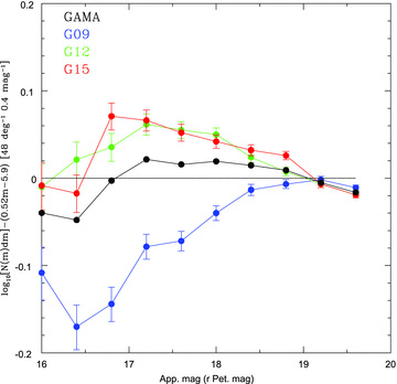
Normalized number-counts as indicated for the three regions and the average. Error bars are based on Poisson statistics suggesting an additional source of error, most likely cosmic (sample) variance between the three GAMA fields. The data become consistent only at rpet > 19 mag.
3 ADDITIONAL IMAGE ANALYSIS PRODUCTS
At this point we have two distinct catalogues: the input catalogue (GamaTiling) used by the tiling algorithm, which defines all viable target galaxies within the GAMA regions, and the combined redshift catalogue (GamaRedshifts), which consists of the pre-existing redshifts and those acquired by the GAMA Team and described in detail in the previous section. Our core catalogues consist of the combination of these two catalogues with three other catalogues containing additional measurements based on the ugrizYJHK imaging data from SDSS DR6 and UKIDSS LAS archives. These additional catalogues are GamaPhotometry, GamaSersic and GamaPhotoz and are briefly described in the sections below (for full details, see Hill et al, 2010a; Kelvin et al., in preparation; Parkinson et al., in preparation). These five catalogues are then combined and trimmed via direct name matching to produce the GAMA Core data set (GamaCore), which represents the combined data from these five catalogues.
3.1 ugrizYJHK-matched aperture photometry (GamaPhotometry)
A key science objective of GAMA is to provide cross-wavelength data from the far-UV to radio wavelengths. The first step in this process is to bring together the available optical and near-IR data from the SDSS and UKIDSS archives. Initially, the GAMA Team explored simple table matching; however. this highlighted a number of issues, most notably differences in deblending outcomes, aperture sizes, and seeing between the SDSS and UKIDSS data sets. Furthermore, as the UKIDSS YJHK data frames are obtained and processed independently in each band by The Cambridge Astronomical Survey Unit group, there is the potential for inconsistent deblending outcomes, inconsistent aperture sizes and seeing offsets between the YJHK bandpasses. Finally, both the SDSS and UKIDSS LAS measure their empirical magnitudes (Petrosian and Kron) using circular apertures (see Petrosian 1976; Kron 1980). For a partially resolved edge-on system, this can result in either underestimating flux or adding unnecessary sky signal increasing the noise of the flux measurement and compounding the deblending issue. To overcome these problems, the GAMA Team elected to re-process all available data to provide matched aperture photometry from u to K using elliptical Kron and Petrosian apertures defined using the r-band data (our primary selection waveband). This process and comparisons to the original data are outlined in detail in Hill et al. (2010a) and described here in brief as follows.
All available data are downloaded and scaled to a uniform zero-point in the strict AB magnitude system (i.e. after first correcting for the known SDSS to AB offset in u and z bands and converting the UKIDSS LAS from Vega to AB, see Hill et al. 2010b for conversions). Each individual data frame is convolved using a Gaussian point spread function (PSF) to yield consistent 2.0 arcsec full width at half-maximum PSF measurements for the intermediate-flux stars. The data frames (over 12 000) are then stitched into single images using the swarp software developed by the TERAPIX group (Bertin et al. 2002), resulting in 27 20-Gb images each of 12 × 4 deg2 at 0.4 × 0.4 arcsec2 pixel sampling. The swarp process removes the background using the method described in SExtractor (Bertin & Arnouts 1996) using a 256 × 256 pixel mesh. SExtractor is then applied to the r-band data to produce a master catalogue and rerun in each of the other eight bandpasses in dual object mode to ensure consistent r-defined Kron apertures (2.5RK, see Kron 1980) from u to K. As the data have been convolved to the same seeing, no further correction to the colours is required. For full details, see Hill et al. (2010a). Fig. 10 shows the u to K data based on archival data (upper panel) and our reanalysis of the archival data (middle panel). The data points are plotted as a colour offset with respect to the z band at their rest wavelengths; hence, the data stretch to lower wavelengths within each band with redshift. As the k- and e-corrections are relatively small in the z band, the data dovetail quite nicely from one filter to the next. The lower panel shows the standard deviation within each log wavelength interval indicating the colour range over which the data are spread. In the U and YJHK bands, the colour distribution is notably narrower for the revised photometry (blue line) over the archival photometry (red line). This indicates a quantifiable improvement in the photometry in these bands over the original archival data with the majority of the gain occurring for objects in more crowded regions. GamaPhotometry contains r-band detections with matched aperture photometry for ∼1.9 million objects, 1 million of which are matched to SDSS DR6 objects. The photometric pipeline is described in full in Hill et al. (2010a) and all SWARP images are made publicly available for downloading at the GAMA website.
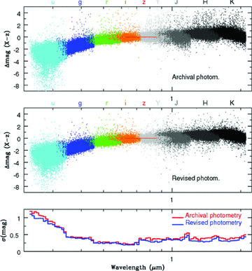
Upper panel: all Main Survey galaxies are plotted according to their colour relative to z band at their observed wavelength. The data points combine to make a global spectral energy distribution for the galaxy population at large – smeared over the redshift range of the survey. Outlier points are typically caused by an erroneous data point in any particular filter. Middle panel: the same plot but using the revised photometry. The lower panel shows the 5σ-clipped standard deviation for these two distributions indicating that in the uYJHK bands the colour distribution is quantifiably narrower reflecting an improvement in the photometry, providing a cleaner data set for detailed SED modelling. Only data with photometry in all bands and with secure redshifts less than 0.5 are shown for clarity.
3.2 Sersic profiles (GamaSersic)

As described in full in Kelvin et al. (in preparation), we use the galfit3 package (Peng et al. 2010) to fit all galaxies to the SDSS DR6 rpet < 22.0 mag. In brief the process involves the construction of comparable swarped images as in Section 3.1 but without Gaussian PSF convolution (raw SWARPS). Instead, the PSF at the location of every galaxy is derived using 20 intermediate-brightness stars from around the galaxy as identified by SExtractor and modelled by the code PSFex (Bertin, private communication). Using the model PSF, the 2D Sérsic profile is then derived via galfit3, which convolves a theoretical profile with the PSF and minimizes the five free parameters. The output Sérsic total magnitude is an integral to infinite radius, which is unrealistic. However, relatively little is known as to how the light profile of galaxies truncates at very faint isophotes with all variants seen (Pohlen & Trujillo 2006).
In order to calculate an appropriate Sérsic magnitude, it is prudent to adopt a truncation radius out to which the Sérsic profile is integrated. For SDSS model magnitudes, exponential (n = 1) profiles were smoothly truncated beyond 3Re and smoothly truncated beyond 7Re for de Vaucouleurs (n = 4) profiles. Here we adopt an abrupt truncation radius of 10Re; for the majority of our data, this equates to an isophotal detection limit in the r band of ∼30 mag arcsec−2 – the limit to which galaxy profiles have been explored. We note for almost all plausible values of n, the choice of a truncation radius of 7Re or 10Re introduces a systematic uncertainty that is comparable or less than the photometric error. Fig. 11 shows a comparison of the three principal photometric methods, with rpet−rKron versus log10(n) (upper panel),  versus log10(n) (middle panel) and
  versus log10(n) (lower panel). Note that it is more logical to compare to log10(n) than n as it appears in the exponent of the Sérsic profile definition (see review of the Sérsic profile in Graham & Driver 2005 for more information). The top panel indicates that our Kron photometry (defined in Section 3.1) reproduces (with scatter) the original SDSS photometry. As described in the previous section, the motivation for rederiving the photometry is to provide elliptical matched apertures in ugrizYJHK. The middle and lower plots show a significant bias between these traditional methods (Petrosian and Kron) and the new Sérsic 10Re magnitude. The vertical lines indicate the location of the canonical exponential and de Vaucouleurs profiles. For normal discs and low-n systems, the difference is negligible. However, for n > 4 systems, the difference becomes significant. This is particularly crucial as the high-n systems are typically the most-luminous and most-massive galaxy systems (Driver et al. 2006). Hence, a bias against this population can lead to serious underestimation of the integrated properties of galaxies, for example, integrated stellar mass or luminosity density (see fig. 21 of Hill et al. 2010a, where a 20 per cent increase in the luminosity density is seen when moving from Petrosian to Sérsic magnitudes). The Sérsic 10Re magnitudes are therefore doing precisely what is expected, which is to recover the flux lost via the Petrosian or Kron photometric systems.
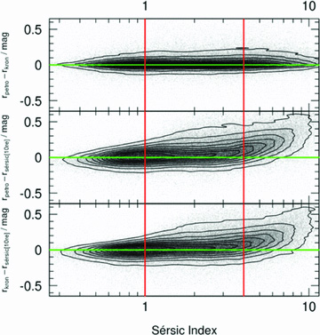
Original SDSS Petrosian magnitudes versus our SExtractor-based Kron magnitudes (top panel), original SDSS Petrosian magnitudes versus our galfit3 Sérsic magnitudes (integrated to 10Re) (middle panel) and our SExtractor Kron versus our galfir3 Sérsic magnitudes (integrated to 10Re) (lower panel). Contours vary from 10 to 90 per cent in 10 per cent intervals.
GamaSersic contains the five parameter Sérsic output for all 1.2 million objects with SDSS DR6 rpet < 22 and full details of the process are described in Kelvin et al. (in preparation). At the present time, we only include in our core catalogues the individual profiles for each object and the r_SERS_MAG_10RE parameter (see Table A2) while final checks are being conducted. We release the total correction to allow for an early indication of the Kron–Total magnitude offset, but caution that these values may change. Similarly, we include for individual objects all profiles with the full Sérsic information specified but again caution that these may change slightly over the next few months as further checks continue. If colour gradients are small, then the r-band Kron to Total magnitude offset given by r_SERS_MAG_10RE can be applied to all filters.
Parameters held in GamaCoreMainSurvey, GamaCoreDR1 and GamaCoreExtraDR1.
| Column | Parameter | Units | Definition |
| 1 | GAMA_IAU_ID | N/A | Unique IAU identifier |
| 2 | GAMA_ID | N/A | Unique six-digit GAMA identifier linked to GAMA’s original SDSS DR6 input catalogue |
| 3 | SDSS_ID | N/A | Sloan Identifier from the SDSS DR6 |
| 4 | RA_J2000 | Degrees | RA taken from the SDSS DR6 |
| 5 | DEC_J2000 | Degrees | Dec. taken from the SDSS DR6 |
| 6 | r_PETRO | AB mag | Extinction-corrected r-band Petrosian flux derived from the SDSS DR6 |
| 7 | Z_HELIO | N/A | Heliocentric redshift (−2 = embargoed, =−0.9 if nQ = 1) |
| 8 | Z_QUALITY | N/A | Confidence on redshift (definite, nQ = 4; reliable, nQ = 3; uncertain, nQ = 2; unknown, |
| nQ = 1; not observed, nQ = 99) | |||
| 9 | Z_SOURCE | N/A | Origin of redshift 1 = SDSS DR6, 2 = 2dFGRS, 3 = MGC, 4 = 2SLAQ-LRG, 5 = GAMA, |
| 6 = 6dFGS, 7 = UZC, 8 = 2QZ, 9 = 2SLAQ-QSO, 10 = NED | |||
| 10 | Z_DATE | N/A | Date of observation if z_SOURCE = 5 (i.e. GAMA), otherwise 99 |
| 11 | Z_SN | N/A | Mean S/N of spectrum if z_SOURCE = 5 (i.e. GAMA), otherwise 99 |
| 12 | Z_ID | N/A | Filename of best available spectrum |
| 13 | PHOT_SOURCE | N/A | Photometric source (rd = r-band defined, sd = self-defined, see Hill et al. 2010a) |
| 14 | u_KRON | AB mag | Extinction u-band Kron magnitude derived from r-band aperture |
| 15 | g_KRON | AB mag | Extinction g-band Kron magnitude derived from r-band aperture |
| 16 | r_KRON | AB mag | Extinction r-band Kron magnitude derived from r-band aperture |
| 17 | i_KRON | AB mag | Extinction i-band Kron magnitude derived from r-band aperture |
| 18 | z_KRON | AB mag | Extinction z-band Kron magnitude derived from r-band aperture |
| 19 | Y_KRON | AB mag | Extinction Y-band Kron magnitude derived from r-band aperture |
| 20 | J_KRON | AB mag | Extinction J-band Kron magnitude derived from r-band aperture |
| 21 | H_KRON | AB mag | Extinction H-band Kron magnitude derived from r-band aperture |
| 22 | K_KRON | AB mag | Extinction K-band Kron magnitude derived from r-band aperture |
| 23 | u_KRON_ERR | AB mag | u -band Kron magnitude error |
| 24 | g_KRON_ERR | AB mag | g -band Kron magnitude error |
| 25 | r_KRON_ERR | AB mag | r -band Kron magnitude error |
| 26 | i_KRON_ERR | AB mag | i -band Kron magnitude error |
| 27 | z_KRON_ERR | AB mag | z -band Kron magnitude error |
| 28 | Y_KRON_ERR | AB mag | Y -band Kron magnitude error |
| 29 | J_KRON_ERR | AB mag | J -band Kron magnitude error |
| 30 | H_KRON_ERR | AB mag | H -band Kron magnitude error |
| 31 | K_KRON_ERR | AB mag | K -band Kron magnitude error |
| 32 | EXTINCTION_r | AB mag | Galactic magnitude extinction in r band |
| 33 | r_SERS_MAG_10RE | AB mag | r -band Sérsic magnitude truncated at 10 half light radii |
3.3 Photometric redshifts (GamaPhotoz)
The GAMA spectroscopic survey is an ideal input data set for creating a robust photometric redshift code that can then be applied across the full SDSS survey region. Unlike most spectroscopic surveys, GAMA samples the entire SDSS r-band-selected galaxy population in an extensive and unbiased fashion to rpet = 19.8 mag – although for delivery of robust photo-redshift to the full depth of the SDSS, it is necessary to supplement GAMA with deeper data. Below we briefly summarize the method, explained in greater detail in Parkinson et al. (in preparation).
We use the Artificial Neural Network code ANNz (Collister & Lahav 2004) with a network architecture of N:2N:2N:1, where N = 6 is the number of inputs to the network (five photometric bands and one radius together with their errors). In order to develop a photo-redshift code valid for the full-SDSS region, we use the ugriz übercal calibration of the SDSS DR7 (Padmanabhan et al. 2008), together with the best of the de Vaucouleurs or exponential half-light radius measurement for each object (Abazajian et al. 2009). Our training set is composed of all GAMA spectroscopic redshifts and zCOSMOS spectroscopic redshift (Lilly et al. 2007), as well as the 30-band COSMOS photometric redshifts (Ilbert et al. 2009). With a redshift error of <0.001, these are as good as spectroscopy when it comes to calibrating five-band photo-redshift from the SDSS alone. The corresponding fractions in the training, validating and testing sets are 81, 4 and 15 per cent, respectively, with over 120k galaxies in total. For COSMOS (and hence zCOSMOS) galaxies, we perform a careful matching to SDSS DR7 objects. This large, complete and representative photo-redshift training set allows us to use an empirical regression method to estimate the errors on individual photometric redshifts. The left-hand panel of Fig. 12 shows that up to zph≈ 0.40 the bias in the median-recovered photo-redshift is less than 0.005/(1 +zph), while beyond it (not shown), the bias is typically within 0.01/(1 +zph). Considering the random errors on the individual estimates, this systematic bias is negligible, while still very well quantified. The right-hand panel of Fig. 12 presents the equivalent plot using SDSS DR7 photometric redshifts, as listed in the Photo-z table of the SDSS Sky Server. In both cases, these plots show only galaxies with rpet < 19.8 mag. This comparison highlights the importance of using a complete and fully representative sample in the training of photometric redshifts.
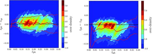
Left-hand panel: GAMA photometric and spectroscopic redshift comparison as a function of the photometric redshift for GAMA galaxies, colour coded as function of galaxy (over-)density. The thick red central line shows the median, while the outer lines delineate the central 68 per cent of the distribution as function of zph. Right-hand panel: same as the left-hand panel, but for the SDSS photometric redshift estimate, extracted from the photo-redshift table in the SDSS DR7.
For an extensive and complete training set, such as GAMA, it is possible to derive a simple and direct method for calculating photo-redshift errors. We estimate the photo-redshift accuracy in a rest-frame colour–magnitude plane with several hundreds of objects per 0.1 × 0.1 mag bin down to rpet = 19.8 mag and typically about 50 objects per 0.1 × 0.1 mag bin down to rpet≈ 21.5 mag. This method provides a robust normally distributed error for each individual object. We note that with this realistic photo-redshift error it is possible to correctly recover the underlying spectroscopic redshift distribution with our ANNz photometric redshifts as illustrated in Fig. 13. It is interesting to note that, without this added error, the raw photo-redshift histogram is actually narrower than the spectroscopic histogram. This makes sense, because photo-redshift calibration yields no bias in true z at given zphot: it is thus inevitable that there is a bias in zphot at given true z, which is strong wherever N(z) changes rapidly; this effect can be seen in operation in the ranges z < 0.05 and 0.3 < z < 0.5. GamaPhotoz contains both photometric redshifts and errors for all systems to rmodel < 21.5 mag and the code is currently being applied across the full SDSS region. We plan to release our prescription for these improved all-SDSS photo-redshift by the end of 2010. In the meantime, we are open to collaborative use of the data: contact [email protected].
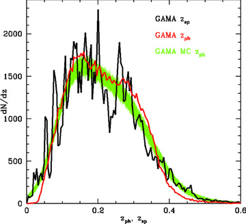
Spectroscopic redshift distribution of GAMA galaxies (black), the corresponding photo-redshift distribution of GAMA galaxies (red) and 1000 Monte Carlo generated photo-redshift distributions, including the Gaussianly distributed photo-redshift error (green).
4 BUILDING AND TESTING THE GAMA CORE CATALOGUES
We can now combine the five catalogues described above to produce the GamaCore catalogue of ∼1 million objects, which contains what we define as our core product to r < 22 mag. Figs 14–16 use this catalogue to illustrate the progression of the redshift survey over the years through the build-up of the cone plots in the three distinct regions. As the survey has progressed, the fidelity with which structure can be resolved and groups identified has increased significantly. In the final maps, the survey is over 98 per cent complete with a near uniform spatial completeness for all three regions, thanks to the ‘greedy’ targeting algorithm (see Robotham et al. 2010). From GamaCore, we now extract three science-ready subsets:
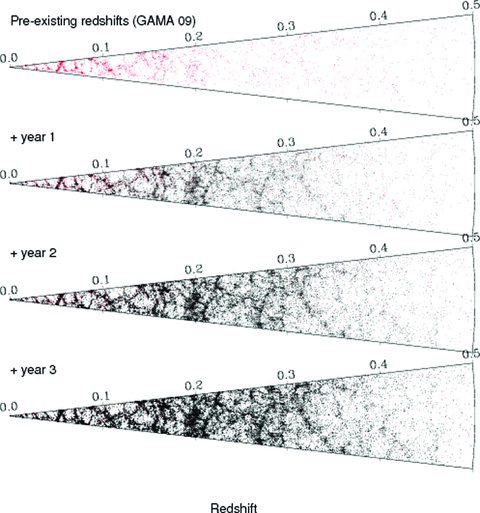
Redshift cone diagram for the GAMA 09 region showing (from top to bottom) pre-existing data, year 1 data release added, year 2 data release added and year 3 data release added.
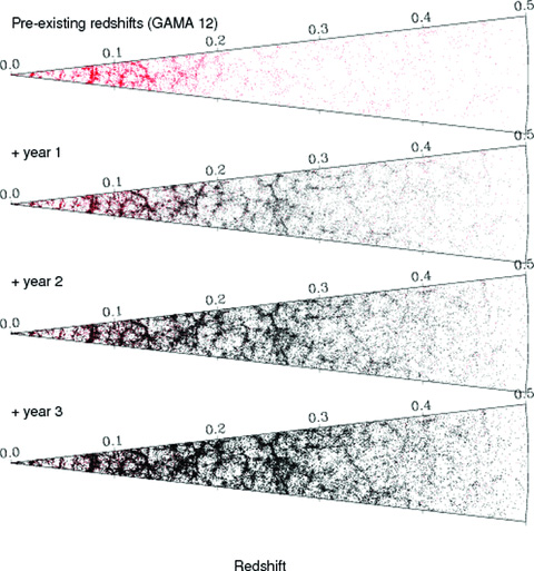
Redshift cone diagram for the GAMA 12 region showing (from top to bottom) pre-existing data, year 1 data release added, year 2 data release added and year 3 data release added.

Redshift cone diagram for the GAMA 15 region showing (from top to bottom) pre-existing data, year 1 data release added, year 2 data release added and year 3 data release added.
GAMA data release 1 (GamaCoreDR1), which includes the majority of spectroscopic data acquired in year 1 with rpet < 19.0 mag and a central strip in G12 (δ± 0
 5) to rpet < 19.8 mag and which forms our primary public data release product at this time.
GAMA Science (GamaCoreMainSurvey), which includes all objects within our main selection limits and suitable for scientific exploitation by the GAMA Team and collaborators.
GAMA-Atlas (GamaCoreAtlasSV), which includes all year 1 and year 2 data with reliable matches to the H-ATLAS science demonstration catalogue as described in Smith et al. (2010) and is currently being used for science exploitation by the H-ATLAS team. For further details and for the H-ATLAS data release, see http://www.h-atlas.org
In the following section, we explore the properties of the two primary catalogues (GamaCoreDR1 and GamaCoreMainSurvey) and do not discuss GamaAtlasSV any further.
4.1 Survey completeness
In Fig. 6, we showed the completeness of the GAMA redshift survey only (i.e. the number of galaxies with redshifts secured by GAMA divided by the GAMA target list). This was given by the number of objects with secure redshifts divided by those targeted during the 3-yr spectroscopic campaign. In Fig. 17, we show the equivalent completeness (i.e. the number of galaxies for which redshifts are known by any source divided by the number of galaxies known in the GAMA regions), but now for the combined data as described in Section 2.8 for our two principal scientific catalogues (GamaCoreDR1 and GamaCoreMainSurvey). This is given by the known redshifts in the GAMA regions divided by the known targets in the GAMA region. The blue regions show the pre-existing redshifts acquired before GAMA commenced and is mainly dominated by the SDSS DR6 with a spectroscopic limit of rpet < 17.77 mag (cf. Table 2). GamaCoreDR1 is shown in green where the main focus in year 1 was to survey objects brighter than rpet = 19 mag with the exception of a central strip in the G12 region (motivated by the desire to assess the completeness function in preparation for year 2 and 3 observations).
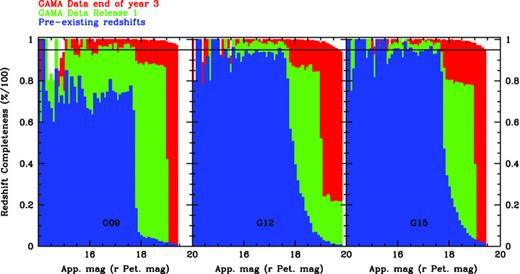
The final completeness of the combined redshift catalogues prior to survey commencing (blue), after GamaCoreDR1 (green) and GamaCoreMainSurvey (red) for G09, G12 and G15 (left-hand to right-hand side), respectively. In all cases, the solid black lines show 95 per cent completeness.
GamaCoreDR1 is relatively complete to rpet < 19.0 mag and the residual spatial bias can be compensated for by using the survey masks provided (see Section 5). After year 3 observations (GamaCoreMainSurvey), one can see 95 per cent or greater completeness in all apparent magnitude intervals with a smooth tapering off from 99 to 95 per cent completeness in the faintest 0.5 mag interval. As all targets without a redshift have now been visually inspected, this fall in completeness is real and obviously needs to be taken into consideration in any subsequent analysis. However, GAMA remains the most-complete survey published to date with the 2dFGRS achieving a mean survey completeness of 90 per cent to bJ = 19.45 mag, SDSS 90 per cent to rpet = 17.77 mag and the MGC 96 per cent to B = 20 mag.
4.2 Survey bias checks
In Fig. 17, we see a small but non-negligible completeness bias with apparent magnitude; hence, it is worth checking for any bias in the obvious parameter space of colour, surface brightness, concentration and close pairs. We explore the first three of these in Fig. 18 for year 1 data (left-hand panels), year 2 data (middle panels) and year 3 data (right-hand panels). The colour indicates the degree of completeness in these 2D planes and the contours show the location of the bulk of the galaxy population. In all three cases, there is no strong horizontal bias that would indicate incompleteness with colour, surface brightness or concentration. This is not particularly surprising, given the high overall completeness of the survey, which leaves little room for bias in the spectroscopic survey, but we acknowledge the caveat that bias in the input catalogue cannot be assessed without deeper imaging data. However, a comparison of single-scan stripe 82 data versus stacked scans suggests no major bias (see Loveday et al., in preparation). Note that in these plots surface brightness is defined by μeff=rpet+ 2.5 log10(2 πab), where a and b are the major and minor half-light radii as derived by galfit3 (see Kelvin et al., in preparation, for details of the fitting process) and concentration is defined by log10(n), where n is the Sérsic index derived in Section 3.2.
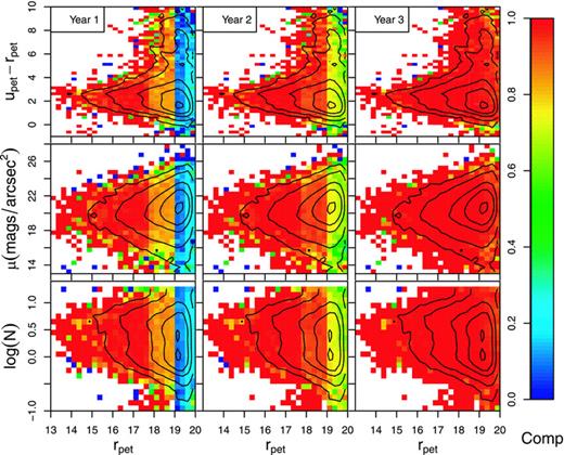
Completeness in the bivariate planes of apparent magnitude and u−r colour (top panels), apparent magnitude and effective surface brightness (middle panels), and apparent magnitude and Sérsic index (bottom panels) for GAMA data after year 1 (left-hand panels), year 2 (middle panels) and year 3 (right-hand panels). Contours show the percentage of galaxies enclosed from out to in, 99, 95, 75, 50 and 5 per cent. Apart from the progression in apparent magnitude over the 3 yr, no other obvious bias is evident.
A major science priority of the GAMA programme is to explore close pairs and galaxy asymmetry (e.g. De Propris et al. 2007). As GAMA is a multipass survey with each region of sky being included in four to six tiles (see Fig. 2), the close pair biases due to minimum fibre separations, which plague the 2dFGRS, SDSS and MGC studies, are overcome. Fig. 19 shows the redshift completeness versus Neighbour Class (NC). The NC of any galaxy is defined (see Baldry et al. 2010) as the number of target galaxies within a 40 arcsec radius. The nominal 2dF fibre-collision radius. The figures shows the progress towards resolving these complexes at the outset and after each year the survey has been operating. All low-NC objects are complete with only a few redshifts outstanding in a small fraction of the higher NC complexes. The data therefore represent an excellent starting point for determining merger rates via close pair analyses.
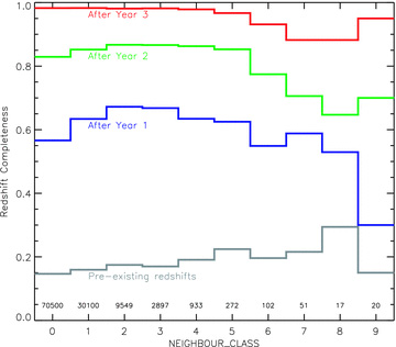
The redshift completeness as a function of NC. NC is defined for each target as the number of other Main Survey targets within 40 arcsec (numbers with each NC value are annotated in the figure). The various lines show the progress in resolving clustered objects at the outset and after each year of observations for the r-limited Main Survey. Note the bias towards NC > 0 after year 1 and year 2 is the result of increasing the priority of clustered targets (Robotham et al. 2010) in order to avoid being biased against NC > 0 after year 3. The final survey has fully resolved almost all close complexes, leaving only a minimal bias when determining merger rates via close pairs: the redshift completeness is >95 per cent for NC ≤ 5.
4.3 Overdensity/underdensity of the GAMA regions
All galaxy surveys inevitably suffer from cosmic variance, more correctly stated as sample variance. Even the final SDSS, the largest redshift survey to date, suffers an estimated residual 5 per cent cosmic variance to z < 0.1 (see Driver & Robotham 2010) – mainly attributable to the ‘Great Wall’ (see Baugh et al. 2004; Nichol et al. 2006). As the GAMA regions lie fully within the SDSS, it is possible to determine whether the GAMA regions are overdense or underdense as compared to the full SDSS over the unbiased redshift range in common (z < 0.1) and relative to each other at higher redshifts where the SDSS density drops due to incompleteness imposed by the rpet < 17.77 mag spectroscopic limit. Fig. 20 shows results with the upper panel showing the density of M*± 1.0 galaxies (defined as M*− 5log h=−20.81 mag) in 0.01 redshift intervals, for a 5000-deg2 region of the SDSS DR7 (blue) and for the three GAMA blocks (as indicated), and the sum of the three regions (black histogram). The k- and e-corrections adopted and the methodology, including the SDSS sample construction, are described in Driver & Robotham (2010), but are not particularly important as we are not exploring trends with z but rather the variance at fixed z. The error bars shown are purely Poisson and so discrepancies larger than the error bars are indicative of cosmic variance induced by significant clustering along the line of sight. The middle and lower panels show the sum of these density fluctuations relative to either the SDSS (middle panel) or the average of the three GAMA fields (lower panel). Note that these panels (middle and lower) now show the density fluctuation out to the specified redshift as opposed to at a specific redshift (top panel), that is, the cosmic variance. We can see that out to z = 0.1 the three GAMA fields are overall 15 per cent underdense with respect to a 5000-deg2 region of the SDSS DR7 (note the volume surveyed by the SDSS comparison region is ∼1.3 × 10⁷h−3 Mpc3). This is extremely close to the 15 per cent predicted from Table 2 of Driver & Robotham (2010). Beyond z = 0.1 one can only compare internally between the three GAMA fields. The inference from Fig. 20 is that for any study at z < 0.2 the cosmic variance between the three regions is significant with G09 in particular being underdense for all redshifts z < 0.2 when compared to the other two regions (note the volume surveyed within the combined GAMA regions to z < 0.2 is ∼2.8 × 10⁶h−3 Mpc3). It is therefore important when considering any density measurement from GAMA data to include the cosmic variance errors indicated in Fig. 20. For example, a luminosity function measured from the G09 region only out to z = 0.1 would need to be scaled up by 1.41 times, etc.
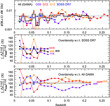
Upper panel: the differential number density of M*± 1.0 mag galaxies in redshift intervals of 0.01. Middle panel: the overdensity of M*± 1.0 mag galaxies out to the specified redshift for the survey indicated by line colour relative to that seen in a 5000-deg2 region of the SDSS DR7. Lower panel: the overdensity of M*± 1.0 mag galaxies out to the specified redshift for the survey indicated relative to that seen over all three GAMA regions.
5 MASKS
For accurate statistical analysis of GAMA, it is essential to have a full understanding of the criteria that define its parent photometric catalogue and also of the spatial and magnitude-dependent completeness of the redshift catalogue. For this purpose, we have defined three functions characterizing this information as a function of the position on the sky and magnitude selection. Here we present briefly the two most important ones, that is, the survey imaging mask function and the redshift completeness mask relative to the main rpet survey limits. The combination of both functions is key for any spatially-dependent measurements based on GAMA data and in particular on GAMA year 1 data. Additional survey completeness masks for other selections (e.g. z, K), or any combination of, are available to the GAMA Team and will be released shortly.
5.1 The imaging mask
We are interested in knowing which regions of the GAMA areas have not been properly covered by the SDSS imaging survey or which should be excluded owing to the presence of bright stars. For that reason, we want to map out SDSS imaging areas containing any of the following information: bleeding pixel, bright star, satellite trail or hole.
First, we create, following the imaging mask information available on the SDSS DR6 website,3 the associated convex polygons, delimiting areas for which imaging information is either not available or could be corrupted (as in the case of bleeding pixels). We primarily use the r-band imaging mask information, as GAMA is nominally an r-band-selected survey, but for completeness we construct all five SDSS imaging masks for the GAMA areas.
The final imaging mask function is then the union of the two separate functions. For ease of use, the imaging masks have been pixelated using an equal-area projection.
5.2 The rpet redshift completeness mask
Normally a simple way to define a redshift success rate would be to make use of the geometry defined by the complete set of 2° fields that were used to tile the survey region for spectroscopic observations. However, due to the tiling strategy adopted in the first year, due to the pre-selection of observing the brightest targets first and due to the much higher number density of galaxies than can be accommodated in a single 2dF, this simple and straightforward approach does not account well enough for the spatial incompleteness of the survey. Therefore, for year 1 data, we had to develop different completeness masks, each defined for a different magnitude limit interval:
For G09 and G15, there are two completeness masks each: one for galaxies brighter than rpet = 19.0 and one for 19.0 ≤rpet < 19.4.
For G12, there are three completeness masks: the same two as for G09 and G15, as well as one for 19.4 ≤rpet < 19.8.
Once the samples for which completeness masks are needed have been defined, one just needs to provide a reasonable definition for the redshift success rate. We choose to tessellate the GAMA regions with a large number of sectors. We incorporate the relevant imaging mask at this stage, by imposing that sectors do not cover any regions masked by the imaging mask. Each sector contains 15–50 galaxy targets and is limited in extent (less than 24 arcmin) and size (less than 225 arcmin2). These conditions are necessary to avoid shot-noise-dominated masks and to guarantee that small-scale information is preserved as much as possible. We note that in the current implementation these sectors are not uniquely defined,4 but once specified any given position on the sky belongs to a unique sector. For each sector, θ, we define the redshift success rate, Rz(θ), for a sample of galaxies within specified magnitude limits, as the ratio of the number of galaxies for which good quality redshifts have been obtained, Nz(θ), to the total number of objects contained in the tiling catalogue, Nt(θ). The redshift completeness of a given sector, Rz(θ), should be clearly distinguished from the redshift completeness of a given 2dF field, cF, since multiple overlapping fields can contribute to a single sector and cF is a measure of the quality of the observing conditions for galaxies observed at the same time.
We present in Fig. 21 the completeness masks for all three regions for GamaCoreDR1 (left-hand panel) and GamaCoreMainSurvey (right-hand panel) to rpet < 19.0. Completeness masks for all regions and different selections are available to the team members and collaborators only at this stage.
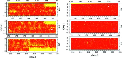
Spatial completeness masks to rpet < 19.0 mag after year 1 (left-hand panel) and year 3 (right-hand panel). The three GAMA regions are shown from top to bottom as G09, G12 and G15. The white regions indicate areas not sampled either due to missing input catalogue data or due to bright stars.
6 GAMA SCIENCE-READY CATALOGUES AND DATA RELEASE 1
The combination of our five input catalogues, as outlined in Section 4, constitutes our core GAMA catalogue of ∼1 million galaxies lying within the GAMA regions and extending to approximately rpet < 22.0 mag. This catalogue has inhomogeneous selection, liable to be incomplete towards the faint-end, along with significant noise in the photometry at the very faint limit and spurious detections. We therefore extract from this data set three science-ready catalogues and one overflow catalogue. These four catalogues along with the complete swarped mosaics of the GAMA regions, associated spectra bundles, images, Sérsic profiles and a variety of data inspection tools (including a MySQL access point) constitute our first data release and are now available at: http://www.gama-survey.org/
6.1 GamaCoreMainSurvey – available from 2012 July 1
The GamaCoreMainSurvey is the GAMA Team’s principal science catalogue and is constructed from GamaCore by removing all objects outside our Main Survey limits as defined in Baldry et al. (2010). These limits are rpet < 19.4 mag in G09 and G15 and rpet < 19.8 mag in G12 (114 441 objects). KKron < 17.6 with rmodel < 20.5 mag (61 393 objects) or zModel < 18.2 with rmodel < 20.5 mag (55 534 objects) and are selected using SURVEY_CLASS > 3 (for a description of the SURVEY_CLASS parameter, see Table 4). This amounts to 119 778 objects in total of which 101 576 are new redshifts provided by GAMA and 18 202 pre-existing. Fig. 17 shows the completeness in the r band; however, similar plots can trivially be constructed in z or K. The spectroscopic completeness (which includes objects not targeted) is 98.2 per cent in r, 99.3 per cent in z and 98.6 per cent in K. The parameters contained in this catalogue are listed in Table A2. As this is our main science catalogue, we place an embargo on its public release until 2012 July 1, but are open to requests for collaboration sent to [email protected].
The SURVEY_CLASS parameter given in GamaTiling. Objects take the higher value if satisfying more than one criterion. All objects with SURVEY_CLASS ≥2 pass the standard star–galaxy separation (see Baldry et al. 2010 for details).
| Value | Number | Fraction Q≥ 3 | Criteria and notes |
| 7 | 59 756 | 0.995 | rpet < 19.0 and Δsg > 0.25 (high priority in year 1) |
| 6 | 54 685 | 0.968 | rpet < 19.4 or rpet < 19.8 in G12 (≥6 for r-limited Main Survey) |
| 5 | 1386 | 0.703 | zmodel < 18.2 (≥5 for SDSS-magnitude-limited Main Survey) |
| 4 | 3951 | 0.879 | KAB < 17.6 (≥4 for Main Survey) |
| 3 | 33 134 | 0.343 | 19.4 < rpet < 19.8 in G09 or G15 (F2 fillers) |
| 2 | 14 861 | 0.196 | gmodel < 20.6 or rmodel < 19.8 or imodel < 19.4 in G12 (F3 fillers) |
| 1 | 1255 | 0.577 | Radio-selected targets (F1 fillers, Ching et al., in preparation) |
| 0 | 822 | 0.394 | 2 ≤ VIS_CLASS ≤4 (see Table 3, or fails star–galaxy separation for rfib < 17) |
6.2 GamaCoreDR1 – available from 2010 June 25
The GamaCoreDR1 is the current GAMA DR 1 catalogue and is constructed from GamaCoreMainSurvey by applying a strict r-band selection of rpet < 19.4 mag in G09 and G15 and rpet < 19.8 mag in G12 (this is implemented by extracting objects with SURVEY_CLASS > 5). While the final GAMA survey is independently r, z and K selected, a strict r-band cut is imposed because observations during year 1 were r-band limited only with the additional cuts coming in in years 2 and 3. Future releases involving year 2 and 3 data will therefore include z- and K-band-selected samples. Selecting on SURVEY_CLASS > 5 yields a catalogue of 114 441 objects spread across the three GAMA regions. Table A2 contains a list of the parameters being released at this time. Redshift information (i.e. quality, S/N, etc.) is provided for all targets, while the redshifts are only provided for year 1 observations above rpet = 19.0 mag (52 324 objects) and for a deeper narrow strip in G12 with Dec. δ=±0 5 to 19.0 < rpet < 19.8 mag (7533 objects). These limits are chosen as they represent our year 1 spectroscopic targeting limits (see Figs 17, 18 and 21, left-hand panels). The redshift release constitutes approximately 50 per cent (59 479 objects; 419 02 GAMA; 17 577 pre-existing) of the entire GAMA data set (or 32.7 per cent of the redshifts acquired by the GAMA Team over the past 3 yr). This data set provides a clean, well-defined, r-band-selected sample suitable for scientific exploitation as shown by Figs 17 and 18. Please note that redshifts outside the specified flux limits or collected after year 1 are currently denoted as Z_HELIO =−2. The redshift quality and S/N information refers to the final best spectrum held in GamaCoreMainSurvey providing advance information as to whether a reliable redshift exists in the larger data base. Requests for individual redshifts for specific objects can be directed to [email protected].
6.3 GamaCoreAtlasSV – available from 2010 June 25
GamaCoreAtlasSV is the subset of objects that have both GAMA and H-ATLAS detection (see Smith et al. 2010 for details of source matching). 1175 objects coexist between the two data sets in a region defined by the geometric overlap between G09 and the H-ATLAS SV region (see Fig. 22), with an approximate area of ∼16.7 deg2. Using the GamaCoreMainSurvey catalogue, we find ∼15 per cent of GAMA Main Survey targets have a H-ATLAS source match. Of these matches, 89 do not have any available redshift, 306 have SDSS redshifts, 792 have GAMA redshifts and one object has a 2SLAQ-QSO redshift. The GAMA redshifts comprise 523 year 1 redshifts, 182 year 2 redshifts and 87 year 3 redshifts. There are no magnitude cuts imposed for GamaCoreAtlasSV and therefore 178 of these redshifts derive from GamaCoreExtra. Note that to extract a homogeneously selected sample, one must trim this catalogue to rpet < 19.4 mag. Table A3 shows the parameters included in this catalogue.
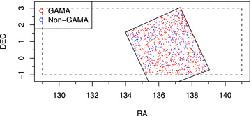
The location of the H-ATLAS science verification region overlaid on the GAMA 9-h region (dotted lines) and showing the location of pre-existing (blue) and new GAMA (red) redshifts within the common region.
Parameters held in GamaCoreAtlasSV.
| Column | Parameter | Units | Definition |
| 1 | GAMA_IAU_ID | N/A | IAU-certified GAMA ID |
| 2 | GAMA_ID | N/A | Unique six-digit GAMA identifier linked to GAMA’s original SDSS DR6 input catalogue |
| 3 | SDSS_ID | N/A | Sloan Identifier from the SDSS DR6 |
| 4 | RA_J2000 | Degrees | RA taken from the SDSS DR6 |
| 5 | DEC_J2000 | Degrees | Dec. taken from the SDSS DR6 |
| 6 | r_PETRO | AB mag | Extinction-corrected r-band Petrosian flux derived from the SDSS DR6 |
| 7 | Z_HELIO | N/A | Heliocentric redshift (−0.9 if nQ = 1) |
| 8 | Z_QUALITY | N/A | Confidence on redshift (definite, nQ = 4; reliable, nQ = 3; uncertain, nQ = 2; unknown, |
| nQ = 1; not observed, nQ = 99) | |||
| 9 | Z_SOURCE | N/A | Origin of redshift 1 = SDSS DR6, 2 = 2dFGRS, 3 = MGC, 4 = 2SLAQ-LRG, 5 = GAMA, |
| 6 = 6dFGS, 7 = UZC, 8 = 2QZ, 9 = 2SLAQ-QSO, 10 = NED | |||
| 10 | Z_DATE | N/A | Date of observation if z_SOURCE = 5 (i.e. GAMA), otherwise 99 |
| 11 | Z_SN | N/A | Mean S/N of spectrum if z_SOURCE = 5 (i.e. GAMA), otherwise 99 |
| 12 | Z_ID | N/A | Filename of the best available spectrum |
| 13 | PHOT_SOURCE | N/A | Photometric source (rd = r-band defined, sd = self-defined, see Hill et al. 2010a) |
| 14 | u_KRON | AB mag | Extinction u-band Kron magnitude derived from r-band aperture |
| 15 | g_KRON | AB mag | Extinction g-band Kron magnitude derived from r-band aperture |
| 16 | r_KRON | AB mag | Extinction r-band Kron magnitude derived from r-band aperture |
| 17 | i_KRON | AB mag | Extinction i-band Kron magnitude derived from r-band aperture |
| 18 | z_KRON | AB mag | Extinction z-band Kron magnitude derived from r-band aperture |
| 19 | Y_KRON | AB mag | Extinction Y-band Kron magnitude derived from r-band aperture |
| 20 | J_KRON | AB mag | Extinction J-band Kron magnitude derived from r-band aperture |
| 21 | H_KRON | AB mag | Extinction H-band Kron magnitude derived from r-band aperture |
| 22 | K_KRON | AB mag | Extinction K-band Kron magnitude derived from r-band aperture |
| 23 | u_KRON_ERR | AB mag | u -band Kron magnitude error |
| 24 | g_KRON_ERR | AB mag | g -band Kron magnitude error |
| 25 | r_KRON_ERR | AB mag | r -band Kron magnitude error |
| 26 | i_KRON_ERR | AB mag | i -band Kron magnitude error |
| 27 | z_KRON_ERR | AB mag | z -band Kron magnitude error |
| 28 | Y_KRON_ERR | AB mag | Y -band Kron magnitude error |
| 29 | J_KRON_ERR | AB mag | J -band Kron magnitude error |
| 30 | H_KRON_ERR | AB mag | H -band Kron magnitude error |
| 31 | K_KRON_ERR | AB mag | K -band Kron magnitude error |
| 32 | EXTINCTION_r | AB mag | Galactic magnitude extinction in r band |
| 33 | r_SERS_MAG_10RE | AB mag | r -band Sérsic magnitude truncated at 10 half light radii |
| 34 | HATLAS_IAU_ID | N/A | H-ATLAS ID as specified by Smith et al. (2010) |
6.4 GamaCoreExtraDR1 – available from 2010 June 25
The GamaCoreExtra catalogue contains information on all objects for which redshifts are known but lie outside the GamaCoreDR1 selection limits. In effect GamaCoreExtra serves as a redshift dumping ground and when combined with GamaCoreMainSurvey or GamaCoreDR1 provides a full record of all objects with known redshifts in the three GAMA regions. This will include pre-existing redshifts at faint magnitudes in the public domain (predominantly from QSO and LRG surveys), along with filler objects targeted during the GAMA campaign. The parameters included are identical to GamaCoreDR1 and therefore also described in Table A2. GamaCoreExtraDR1 is an identical copy of GamaCoreExtra except with the GAMA redshifts embargoed until a later release. GamaCoreExtra is highly inhomogeneous and volatile as additional redshifts come to light and essentially forms the starting point for any extension to the GAMA survey. Currently, it contains ∼16k galaxies of which ∼0.5k are pre-existing and ∼15.5k have been acquired during GAMA observations. Requests for access to individual redshifts or redshifts for specified subregions should be directed to [email protected].
6.5 Future plans
The three science-ready catalogues described in the previous sections are shown in Fig. 23 in the AB r-band magnitude (Mr− 5log h) versus redshift (z) plane (main panel), along with the collapsed N(z) and N(Mr) distributions (upper left-hand and right-hand panels, respectively). The absolute magnitudes are calculated using k-corrections derived from the GAMA u to K photometry, total throughput (including atmosphere) temperature adjusted filter transmission curves and the kcorrect software package (Blanton & Roweis 2007). The figure is intended to provide a rough indication of the parameter range being explored with L* galaxies routinely detected to z≈ 0.3 and objects as faint as Mr=−12 mag being recovered at z > 0.01. In future papers, we will explore more comprehensively the completeness of the initial input catalogue (GamaTiling) in the bivariate brightness distribution plane (BBD; Hill et al. 2011) through a detailed BBD-analysis (see Driver et al. 2005), as well as through comparisons to deeper and higher spatial resolution data.
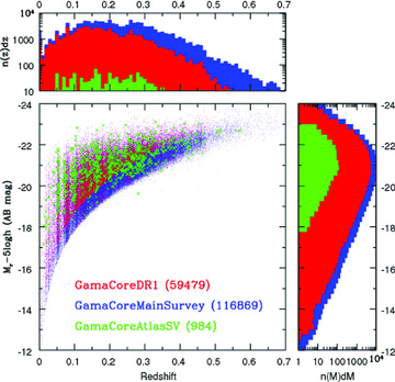
Main panel: the absolute magnitude versus redshift plane for the three science-ready catalogues (as indicated). Upper left-hand panel: the distribution collapsed in redshift. Right-hand panel: the distribution collapsed in absolute magnitude.
In the near term, the GAMA Team will be producing a number of extended data products or data management units (DMUs), which include spectral line analysis via gandalf/ppxf (Cappellari & Emsellem 2004; Sarzi et al. 2006) and stellar population model fits (Thomas, Maraston & Bender 2003; Maraston 2005), bulge–disc decomposition via galfit3, stellar masses and revised photometric redshifts via interest, environmental markers and group catalogues. These data products will be outlined in more detail in our next data release later in the year (Liske et al., in preparation). Within the next 3–5 yr we expect to ingest additional data sets from GALEX, Herschel, WISE, GMRT, VISTA, VST and ASKAP as well as expand our core AAT programme to cover a larger area of ∼400 deg2 to rSersic < 19.8 mag. In due course, DMUs on multiwavelength spectral energy distribution (SED) and H i modelling will provide dust mass/temperature measurements, and gas and dynamical mass measurements.
7 SUMMARY
The GAMA basic data including GAMA and pre-GAMA spectra and redshifts, GAMA swarp-processed images in ugrizYJHK, u to K matched aperture photometry and corrections to total magnitudes are now available at http://www.gama-survey.org/. GAMA Data Release 1 (GamaCoreDR1) data are publicly available via a download page immediately and the full catalogue (GamaCoreMainSurvey) is available for use by the GAMA Team and collaborators. In addition, we make publicly available a catalogue (GamaCoreAtlasSV) including year 2 data for the H-ATLAS science verification region, which form the basis for a number of H-ATLAS science verification papers.
Data inspections tools, including a MySQL tool and direct data inspection toolkit, are provided and will be developed further in due course. The sum of year 1, 2 and 3 data constitutes GAMA Phase I, which is now complete having utilized archival data from the SDSS, UK Infrared Deep Sky Survey and NASA ExtraGalactic Data base (NED), and an initial allocation of 66 nights of AAT time. Value-added data products will be released from 2011 January 1 and regularly thereafter. GAMA Phase II is now underway and aims to add in additional area coverage as well as to extend the depth of the survey. The community is encouraged and invited to contact the team for early access to GamaCoreMainSurvey. The contents of this catalogue are described in Table A2.
Note that from 2010 July 1 the Anglo-Australian Observatory (AAO) has been renamed the Australian Astronomical Observatory (AAO) (see Watson & Colless 2010).
This could be achieved by making each target galaxy the centre of a subsector and then increasing the radius of all subsectors and creating sectors by the merger of overlapping subsectors.
First and foremost we would like to thank the staff of the former Anglo-Australian Observatory (now Australian Astronomical Observatory) for the the smooth running of the telescope and AAOmega during these observations and the funding support we have received from the STFC and the ARC.
Funding for the SDSS and SDSS-II has been provided by the Alfred P. Sloan Foundation, the Participating Institutions, the National Science Foundation, the US Department of Energy, the National Aeronautics and Space Administration, the Japanese Monbukagakusho, the Max Planck Society, and the Higher Education Funding Council for England. The SDSS website is http://www.sdss.org/. The SDSS is managed by the Astrophysical Research Consortium for the Participating Institutions. The Participating Institutions are the American Museum of Natural History, Astrophysical Institute Potsdam, University of Basel, University of Cambridge, Case Western Reserve University, University of Chicago, Drexel University, Fermilab, the Institute for Advanced Study, the Japan Participation Group, Johns Hopkins University, the Joint Institute for Nuclear Astrophysics, the Kavli Institute for Particle Astrophysics and Cosmology, the Korean Scientist Group, the Chinese Academy of Sciences, Los Alamos National Laboratory, the Max-Planck-Institute for Astronomy, the Max-Planck-Institute for Astrophysics (MPA), New Mexico State University, Ohio State University, University of Pittsburgh, University of Portsmouth, Princeton University, the United States Naval Observatory and the University of Washington.
The UKIDSS project is defined in Lawrence et al. (2007). The UKIDSS uses the UKIRT Wide Field Camera (Casali et al. 2007). The photometric system is described in Hewett et al. (2006) and the calibration is described in Hodgkin et al. (2009). The pipeline processing and science archive are described in Irwin et al. (2009, in preparation) and Hambly et al. (2008). We have used data from the 4th data release.
This research has made use of the NED, which is operated by the Jet Propulsion Laboratory, California Institute of Technology, under contract with the National Aeronautics and Space Administration.
The MGC consists of imaging data from the Isaac Newton Telescope and spectroscopic data from the AAT, the ANU 2.3-m, the ESO New Technology Telescope, the Telescopio Nazionale Galileo and the Gemini North Telescope. The survey has been supported through grants from the Particle Physics and Astronomy Research Council (UK) and the Australian Research Council (AUS). The data and data products are publicly available at http://www.eso.org/~jliske/mgc/ or on request from J. Liske or S. P. Driver.
Finally, we would like to acknowledge the use of topcat, stilts, SExtractor, swarp, PSFex, galfit3 and aladin astronomical software packages and the r data analysis package.
REFERENCES
Appendix
APPENDIX A: GAMA CATALOGUES
The four principal GAMA catalogues formed at this time are GamaTiling, GamaCoreMainSurvey, GamaCoreDR1 and GamaCoreAtlasSV. The parameters contained in these catalogues and their explanations are shown in Tables A1–A3.
Parameters held in GamaTiling.
| Column | Parameter | Units | Definition |
| 1 | GAMA_ID | N/A | Unique six-digit GAMA identifier linked to GAMA’s original SDSS DR6 input catalogue |
| 2 | SDSS_ID | N/A | Sloan Identifier from the SDSS DR6 |
| 3 | RA_J2000 | Degrees | RA taken from the SDSS DR6 |
| 4 | DEC_J2000 | Degrees | Dec. taken from the SDSS DR6 |
| 5 | r_FIBREMAG | AB mag | Fibre magnitude |
| 6 | r_PETRO | AB mag | Extinction-corrected r-band Petrosian flux derived from the SDSS DR6 |
| 7 | u_MODEL | AB mag | Extinction-corrected model u mag from the SDSS DR6 |
| 8 | g_MODEL | AB mag | Extinction-corrected model g mag from the SDSS DR6 |
| 9 | r_MODEL | AB mag | Extinction-corrected model r mag from the SDSS DR6 |
| 10 | i_MODEL | AB mag | Extinction-corrected model i mag from the SDSS DR6 |
| 11 | z_MODEL | AB mag | Extinction-corrected model z mag from the SDSS DR6 |
| 12 | NUM_GAMA_SPEC | N/A | Number of spectra available for this object |
| 13 | r_SB | AB mag arcsec−2 | SDSS Petro half-light r-band surface brightness |
| 14 | SG_SEP | mag | SDSS r_psf-r_model star–galaxy separation parameter |
| 15 | SG_SEP_JK | mag | GAMA Auto J−K – f_locus star–galaxy separation parameter |
| 16 | K_KRON_SELECTION | AB mag | Extinction-corrected K magnitude used for selection (old) |
| 17 | TARGET_FLAGS | Bit | Bitwise target criteria (see GAMA website) |
| 18 | SURVEY_CLASS | N/A | Survey class (see Table 4) |
| 19 | PRIORITY_CLASS | N/A | Priority class (see GAMA website) |
| 20 | NEIGHBOUR_CLASS | N/A | Number of Main Survey neighbours within 40 arcsec (see Fig. 19) |
| 21 | MASK_IC_10 | N/A | Mask value 0.0–1.0 around V < 10 mag stars (see Baldry et al. 2010) |
| 22 | MASK_IC_12 | N/A | Mask value 0.0–1.0 around V < 12 mag stars (see Baldry et al. 2010) |
| 23 | VIS_CLASS | N/A | Visual classification (see Baldry et al. 2010 and Table 3) |
| 24 | VIS_CLASS_USER | N/A | Initials of visual classifier for VIS_CLASS |
