


Abstract
We present an analysis of the properties of the lowest Hα-luminosity galaxies (LHα≤ 4 × 1032 W; SFR < 0.02 M⊙ yr−1, with SFR denoting the star formation rate) in the Galaxy And Mass Assembly survey. These galaxies make up the rise above a Schechter function in the number density of systems seen at the faint end of the Hα luminosity function. Above our flux limit, we find that these galaxies are principally composed of intrinsically low stellar mass systems (median stellar mass = 2.5 × 10⁸ M⊙) with only 5/90 having stellar masses M > 1010 M⊙. The low-SFR systems are found to exist predominantly in the lowest-density environments (median density ∼0.02 galaxy Mpc−2) with none in environments more dense than ∼1.5 galaxy Mpc−2. Their current specific SFRs (SSFRs; −8.5 < log [SSFR (yr −1)] < −12) are consistent with their having had a variety of star formation histories. The low-density environments of these galaxies demonstrate that such low-mass, star-forming systems can only remain as low mass and form stars if they reside sufficiently far from other galaxies to avoid being accreted, dispersed through tidal effects or having their gas reservoirs rendered ineffective through external processes.
1 INTRODUCTION
Recent investigations into the evolutionary properties of galaxies have established that the distribution of galaxy colours exhibits a strong bimodality, separating red, quiescent early-type galaxies, with little ongoing star formation, from a blue sequence of star-forming spiral galaxies (e.g. Kauffmann et al. 2003; Baldry et al. 2006; Blanton 2006; Driver et al. 2006). This bimodality can be interpreted in terms of the star formation history (SFH) and stellar mass content (e.g. Tinsley 1968) with the stars in the most-massive galaxies having formed quickly a long time ago and less-massive galaxies still forming stars today.
The current star formation of a galaxy can be traced through its Hα luminosity as this emission gives a direct probe of the young massive stellar population (Kennicutt 1998). The Galaxy and Mass Assembly (GAMA1; Driver et al. 2009, 2011) survey has to date obtained optical spectra for ∼120 000 galaxies in the nearby Universe (z < 0.5). GAMA's deep spectroscopic observations [r < 19.8; 2 mag fainter than the Sloan Digital Sky Survey (SDSS); York et al. 2000] and wide-area sky coverage (three 48-deg2 regions) provide an excellent sample with which to analyse the current star formation rates (SFRs) of a large sample of galaxies, down to very low stellar masses. Gunawardhana et al. (in preparation) have used early data from GAMA to establish that there is a significant increase in the number densities of Hα-emitting galaxies at very low luminosities (Hα luminosities <2.5 × 1032 W, H0 = 100 km s−1 Mpc−1) such that a Schechter function is a poor fit at these luminosities. This has also been observed by Westra et al. (2010) with the Smithsonian Hectospec Lensing Survey.
Characterizing the faint end of the Hα luminosity function is important as both Lee et al. (2007) and Bothwell, Kennicutt & Lee (2009) have found that there is a broadening of the star formation distribution to extremely low SFRs in low-mass as well as high-mass galaxies from their analysis of Hα-derived SFRs for galaxies within 11 Mpc. The broadening of the star formation distribution in high-mass galaxies is due to the cessation of star formation. However, the broadening for low-mass galaxies is an open question with two potential resolutions. First, that the cause of this range is due to a change in the dominant physical process that regulates star formation. These galaxies are generally of low mass and such galaxies have shallow potential wells. They are therefore subject to many processes that are negligible in higher mass systems. Secondly, the possibility that, at low luminosities, the SFR is not being traced as closely by the Hα luminosity due to the existence of fewer young stars, meaning that the initial mass function (IMF) is not fully sampled in these systems. Meurer et al. (2009) and Lee et al. (2009) find that the Hα luminosity underestimates the SFR relative to the far-UV luminosity in dwarf galaxies and that this could be the result of a steeper IMF for galaxies with lower SFRs, for which there is growing theoretical (e.g. Weidner & Kroupa 2005) and observational evidence (Hoversten & Glazebrook 2008; Gunawardhana et al., in preparation).
In this paper, we investigate the characteristics of the low-Hα-luminosity galaxies that comprise the upturn in the Hα luminosity function. We investigate their stellar masses to determine whether the low Hα luminosities are from low-mass galaxies with high specific SFRs (SSFRs) or massive galaxies with low SSFRs and find that these are generally low-mass systems with high SSFRs. We examine how much of the increase in number densities seen at low stellar masses (<3 × 10⁸ M⊙; Baldry, Glazebrook & Driver 2008) in the galaxy stellar mass function is due to these systems and find that they do not contribute significantly. We also use the wide area of the GAMA survey to investigate what environment these low-star-forming galaxies are found in and conclude that they are only found in low-density environments.
The layout of this paper is as follows. We describe the construction of the sample in Section 2. In Section 3, we describe the observed properties, SFRs and environmental density of the sample, and discuss our findings in Section 4. Throughout this paper, we assume a Hubble constant of H0 = 70 km s−1 Mpc−1 and an ΩM = 0.3, ΩΛ = 0.7 cosmology. All magnitudes are given in the AB system. We use a Salpeter IMF in our derivations of stellar masses and SFRs for convenience, but recognize that quantitative values may need to be scaled to a more realistic IMF.
2 DATA
The GAMA survey is using wide-field survey facilities to study galaxy formation and evolution over a range of wavelengths. GAMA brings together data from the 3.9m Anglo-Australian Telescope (AAT), the United Kingdom InfraRed Telescope (UKIRT), the Very Large Telescope Survey Telescope (VST), the Visible and Infrared Survey Telescope for Astronomy (VISTA), the Australian Square Kilometre Array Pathfinder (ASKAP), the Galaxy Evolution Explorer (GALEX) and Herschel space telescopes. To date ∼120 000 galaxies in three 48-deg2 regions of sky have been observed (Driver et al. 2009, 2011). Here we use data from the first two years of GAMA optical spectroscopic observations undertaken with the dual-arm AAOmega spectrograph (Sharp et al. 2006) at the AAT. The GAMA input catalogue is described in detail in Baldry et al. (2010) and the spectroscopic tiling of those sources in Robotham et al. (2010). In summary, spectroscopic targets were initially selected from the SDSS Data Release 6 (Adelman-McCarthy et al. 2008) to Galactic-extinction-corrected, Petrosian magnitude limits of r < 19.4 mag in two fields and r < 19.8 mag in one field. The input catalogue includes an explicit low surface brightness limit to aid artefact removal, μr,50 > 15 mag arcsec−2, where μr,50 is the effective r-band surface brightness within the half-light radius. The targets were observed with the 580V and 385R AAOmega gratings giving an observed wavelength range of ∼3700–8900 Å and spectral resolution of 3.2 Å full width at half-maximum. Hα is within the observed wavelength range to redshifts z∼ 0.35. The spectra are extracted with 2dfdr which undertakes a first-order curvature correction and flux calibration in order to accurately splice the spectra from the blue and red arms of the spectrograph. The spectra are then sky subtracted following Sharp & Parkinson (2010) and redshifts determined with runz (Saunders, Cannon & Sutherland 2004). In the first two years of GAMA data, there are 81 274 GAMA redshifts with quality values Q≥ 3 (i.e. regarded as a secure redshift).
The standard strong optical emission lines are measured from each flux-calibrated spectrum. This is done assuming a single Gaussian approximation, fitting for a common velocity and linewidth within an adjacent set of lines (e.g. Hβ and the [O iii] doublet and separately, Hα and the [N ii] doublet) whilst simultaneously fitting the continuum local to the set of lines with a straight-line fit. We measure the limit to which our Hα fluxes are robust from a self-consistent error estimation of emission-line fits (Acosta-Pulido et al. 1996). Since the ratios of the fluxes of emission-line doublets are purely set by quantum mechanics, we use measurements of the [O iii] and [N ii] doublet fluxes to measure the flux at which the ratio is no longer accurate to within 10 per cent. For a single line, this then translates to a flux limit of 3 × 10⁻¹⁶ erg s−1 cm −2. We determine the limit to which our Hα fluxes are complete (i.e. 1 × 10⁻¹⁵ erg s−1 cm −2) from the number counts of our measurements. We make no attempt to construct a complete, volume- or mass-limited sample as obtaining a reasonable range in luminosity or redshift ends up in excluding the low-Hα-flux systems that we are studying. Instead we take advantage of the fact that we can detect systems to these faint levels to explore the nature of some of the most extreme systems in the GAMA sample.
A significant increase in the number densities of Hα-emitting galaxies at very low luminosities is observed in the lowest-redshift bin of the GAMA Hα luminosity function (z≤ 0.13; Gunawardhana et al., in preparation). We therefore focus on galaxies within this redshift range. There are 13 228 GAMA galaxies with Q≥ 3 and 0.002 < z < 0.13 (henceforth referred to as the Whole sample for the purposes of this analysis) and of these, 9623 galaxies have Hα fluxes above our flux limit. We also require that Hβ is measured as it is necessary for dust corrections described later. As Hβ is a significantly weaker emission line, we only require that Hβ is measured, rather than imposing a flux limit, in order not to discard weak-line systems (Cid Fernandes et al. 2010). As we are studying the star-forming properties of this sample, we remove 707 active galactic nuclei following the diagnostic relationships from Kewley et al. (2001). These relationships rely on four emission lines. If we do not have measurements for all four, then we use the two-line diagnostics. If we do not have both lines for the two-line diagnostic, then the galaxy is classified as ‘uncertain’, but remains in the sample to prevent discarding weak-line systems. Using the Kewley et al. (2001) diagnostics only removes four galaxies from the final low-Hα-luminosity sample and does not change any of our conclusions. This leaves a sample of 8916 galaxies.
At redshifts below z∼ 0.02, peculiar velocities are a significant fraction of the measured recessional velocity. This can lead to distance errors of a factor of 2 or more when assuming pure Hubble flow (e.g. Masters, Haynes & Giovanelli 2004). It is therefore important to include local variations from the cosmic microwave background (CMB) frame. We use the GAMA peculiar velocity corrections which are calculated by applying the Tonry et al. (2000) multi-attractor flow model which provides a parametric model for the local velocity field, from z∼ 0.002 (below which the stellar contamination arises) to z∼ 0.02. From 0.02 < zCMB < 0.03, the peculiar velocity corrections are linearly tapered to zero by maximizing the probability density of the corrections and above z∼ 0.03, a pure zCMB is invoked.
We calculate intrinsic galaxy luminosities using GAMA g, r, i magnitudes measured in r-band-defined elliptical Kron apertures (Hill et al. 2011). These magnitudes are corrected for Galactic extinction according to the dust maps of Schlegel, Finkbeiner & Davis (1998) and K-corrected to a redshift z = 0 using the kcorrect V4_1_4 code of Blanton & Roweis (2007) such that Mx=mx− 5 log10[DL(Mpc)]− 25 −Kx. r-band magnitudes re-computed for GAMA are not available for 418 galaxies. These missing magnitudes are generally either due to a SExtractor detection failure or due to a particularly low surface brightness source (Hill et al. 2011). This leaves a sample of 8666 galaxies (henceforth referred to as the Main sample).
2.1 Low-Hα-luminosity sample
From the Main sample of 8693 galaxies, we select the least Hα -luminous galaxies above the flux limit of 3 × 10⁻¹⁶ erg s−1 cm−2 up to the luminosity at which the upturn in the Hα luminosity function is observed (Westra et al. 2010; Gunawardhana et al., in preparation): 2 × 1030≤LHα≤ 4 × 1032 W. The upper limit is equivalent to a SFR of 0.02 M⊙ yr−1, significantly less than the rate observed in the Milky Way of ∼1 M⊙ yr−1 (Robitaille & Whitney 2010).
As these galaxies are approaching the edge of the GAMA selection criteria, SDSS thumbnail images and AAT spectra were compiled for each galaxy and visually inspected to check for discrepancies. The GAMA catalogue is derived from an automated procedure applied to the SDSS and UKIDSS (Baldry et al. 2010). In certain cases, sources were visually checked and given the classification VIS_CLASS = 3 if the object, such as an H ii region, was part of a larger system. These are not included in our sample. In addition, we rejected a further two sources with stars less than 2 arcsec away (as the spectra are contaminated by those stars) and three sources which were H ii regions not previously identified. This leaves a sample of 90 galaxies with 0.002 < z < 0.13 and SFR < 0.02 M⊙ yr−1 (henceforth referred to as the low-LHα sample). The redshift distribution of the low-LHα sample with respect to the Main sample is illustrated in Fig. 1. The effects of our Hα flux limit and Hβ selection are also illustrated.
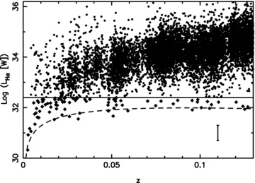
Distribution of Hα luminosity, LHα, with redshift for the Main sample (star-forming galaxies with 0.002 < z < 0.13). Gaps in the distribution are primarily due to large-scale structure at the low-redshift end and are due to the Hα line passing through the Fraunhofer OH atmospheric absorption bands at higher redshifts. The solid line indicates the cut made to select the lowest-Hα-luminosity galaxies. The flux limit of our observations is indicated by the dashed line. The median 1σ error on the Hα luminosity is given in the bottom right-hand corner.
We describe the physical and star formation properties of these galaxies in more detail in the next section.
3 PHYSICAL AND STAR FORMATION PROPERTIES
In order to understand the physical and star formation characteristics of these galaxies in more detail, we examine their optical spectra and multicolour images. We show the optical spectra (from the AAT) and multicolour images (from the SDSS) for two galaxies, illustrative of the low-LHα sample in Fig. 2. These clearly indicate that our selection criteria of low Hα emission identifies diffuse, blue, emission-line galaxies.
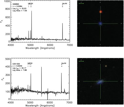
AAOmega spectra (with prominent emission lines marked) and SDSS multicolour images of (in each panel) GAMA galaxies: G69890 and G321325. Names, redshifts, Hα luminosities (W) and stellar masses (M⊙) are given in each panel. The scale bar given in the images corresponds to 5 arcsec, at the redshifts of these systems that is equivalent to 0.8 kpc (G69890) and 0.5 kpc (G321325).
In Fig. 3, we compare the distribution of distances and Hα luminosities for the low-LHα sample with galaxies from Hα imaging surveys of the Local Volume: the 11 Mpc Hα and Ultraviolet Galaxy Survey (11HUGS; Kennicutt et al. 2008) and the Hα Galaxy survey (HαGS; James et al. 2004) which extends to z∼ 0.01. Fig. 3(a) emphasizes the much larger distance scale probed by the GAMA sample. Our sample is the most distant of the three and Fig. 3(b) shows that we find low Hα luminosities similar to the HαGS sample and to the majority of the significantly nearer 11HUGS sample. This suggests that these are some of the most-distant, low-Hα-luminosity galaxies studied.
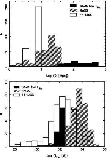
Distribution of low-LHα sample properties compared to other Hα imaging surveys of the Local Volume, as a function of (a) Distance, D and (b) Hα luminosity, LHα.
We compare the colours of these galaxies to those from the New York University (NYU) re-analysis of SDSS low-redshift data: the NYU Value-Added Galaxy Catalogue (NYU-VAGC DR4; 10 < Distance (Mpc h−1) < 150; Blanton 2006) in Fig. 4. The GAMA data are clearly sampling lower luminosities than the majority of the NYU-VAGC low-redshift galaxies. Most are of a similar colour to the ‘blue cloud’ of star-forming galaxies (i.e. g−r < 0.55) showing that these low-Hα-luminosity galaxies follow similar colour relationships to more massive star-forming galaxies. There are a few galaxies on the red sequence and these are some of the more massive galaxies of our sample.
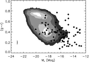
(g−r) colour–magnitude relation. The contours indicate the number density of low-redshift NYU-VAGC galaxies. The low-LHα sample is indicated by the diamonds and can be seen to generally lie on the blue cloud (i.e. g−r < 0.55), with lower luminosities and blue colours. Those in the red sequence are the most massive of the GAMA sample. The median 1σ errors on the magnitudes and colours are given in the bottom left-hand corner.
We examine the size of these galaxies in Fig. 5 using the effective radius (containing half of the flux) from a Sérsic fit to the r-band data. These galaxies are remarkably compact with all having half-light radii ≤1.2 kpc. This result is unchanged if we use the SDSS r50 radius which measures the radius containing 50 per cent of the Petrosian flux.
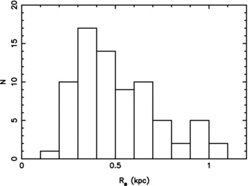
Histogram of Sérsic r-band effective radii, Re. In the low-LHα sample, all have low half-light radii ≤1.2 kpc.
Of primary interest to this analysis are the masses of these galaxies. We use total stellar masses calculated from fits to the u, g, r, i, z spectral energy distribution using the Bruzual & Charlot (2003) stellar population models, assuming a Chabrier (2001) IMF (Taylor et al., in preparation). We adjust these to the Salpeter IMF used here by adding ∼0.2 dex. The distribution of stellar masses with redshift with respect to the Main sample is illustrated in Fig. 6. It is clear that our low-LHα sample is of very low mass at low redshifts, but has increasingly higher masses at higher redshifts. In general we find that these galaxies have low stellar masses; however, five have stellar masses M≥ 1010 M⊙. The median stellar mass of the low-Hα-luminosity sample is 2.5 × 10⁸ M⊙, roughly that of the Small Magellanic Cloud. This is a result of our flux limit, as will be seen in the next section.
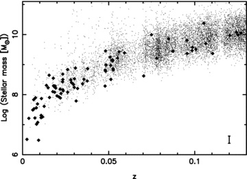
Distribution of the stellar mass with redshift for the Main sample (star-forming galaxies with 0.002 < z < 0.13). The diamonds indicate the low-LHα sample. The formal uncertainty on the stellar masses is 0.12 dex and is indicated by the error bar in the bottom right-hand corner.
The galaxies that make up the upturn in the Hα luminosity function are of similar stellar mass to those that form the increase in the number density seen in the galaxy stellar mass function at stellar masses ≤ 3 × 10⁸ M⊙ (Baldry et al. 2008). To examine the contribution of these low star formation galaxies to the upturn in the stellar mass function, we show the fraction of galaxies classified as having low-Hα luminosity as a function of stellar mass <3 × 10⁸ M⊙ in Fig. 7. As the stellar mass decreases, the low-Hα-luminosity sample is an increasing fraction of the Whole galaxy population and the low star formation galaxies form the largest fraction of the mass function at stellar masses ∼107 M⊙. However, the small numbers of low-Hα luminosity galaxies mean that this is not statistically significant. At higher masses, galaxies with higher SFRs dominate the mass function. The upturn observed in the Hα luminosity function is not cleanly responsible for the upturn observed in the galaxy stellar mass density at the lowest stellar masses. We investigate the SFHs of these galaxies with respect to their stellar masses in the next section.
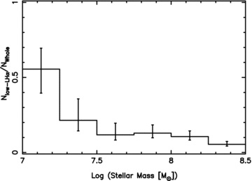
Fraction of the low-LHα sample as a function of the Whole sample (all galaxies with 0.002 < z < 0.13), in bins of stellar mass. The error bars indicate the 1σ confidence intervals on the binomial population proportions (Cameron 2010).
3.1 Star formation histories
In Section 1, we stressed the importance of the SFH on the observed properties of galaxies. To first order, we can characterize the SFH using the SSFR. It is defined as the ratio of the current SFR to the stellar mass formed to date and is closely related to Scalo's stellar birthrate parameter, b (Kennicutt, Tamblyn & Congdon 1994). The SSFR gives a measure of whether the current star formation activity is typical of the past star formation activity [i.e. a constant SFR; log(SSFR) ∼−10, b∼ 1], the current SFR is elevated over the past [i.e. starbursting; log(SSFR) > −10, b≫ 1] or is reduced with respect to the past [i.e. quiescent; log(SSFR) < −10, b≪ 1] and has units of inverse time. Previous analyses have shown that star-forming galaxies preferentially lie on a SSFR sequence with mass, such that the SSFR of low-mass galaxies is higher than that for high-mass galaxies (e.g. Brinchmann et al. 2004; Noeske et al. 2007; Schiminovich et al. 2007). Galaxies in the Local Volume are also observed to lie on the SSFR–mass sequence (Bothwell et al. 2009).
We calculate SFRs from the corrected Hα luminosity using the relationship given by Kennicutt (1998), that is, SFR (M⊙ yr−1) =LHα(W)/1.27 × 1034.
The SSFR–stellar mass relationship is shown in Fig. 8. The SSFR consistent with a constant SFH over a Hubble time (i.e. b∼ 1) is indicated by the dashed line. The SSFR equivalent to our lower flux limit at the median redshift of our sample (z∼ 0.03) is indicated by the dot–dashed line. Our sample selection effectively selects galaxies at the limit in the SSFR–stellar mass relationship. However, the range of masses encompassed by our sample results in a range of SSFRs, consistent with a range of SFHs from quiescent to bursty, depending on their stellar mass. Our flux limit prevents us from observing galaxies with lower SSFRs; however, Hα imaging surveys observe galaxies with the SSFR below our flux limit at these masses (e.g. Kennicutt et al. 1994; Lee et al. 2007; Bothwell et al. 2009). The range of SFHs present for these galaxies is therefore likely to be larger than the distribution we observe at the lowest stellar masses we probe. It is also likely that there are more massive galaxies with similarly low SFRs, as have been observed by the GALEX (e.g. Jeong et al. 2009; Schiminovich et al. 2010). This suggests that a simple relationship between the SSFR and mass may be less warranted and may require more examination of the selection effects involved (e.g. Stringer et al. 2011).
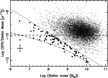
SSFR (SFR/stellar mass) as a function of the stellar mass for the Main sample (star-forming galaxies with 0.002 < z < 0.13). The dashed line indicates the b∼ 1 line for a constant SFH over a Hubble time. The dot–dashed line indicates the Hα flux limit of our data. The dotted line indicates the upper Hα-luminosity limit of our sample. The lowest-Hα-luminosity sample is indicated by the diamonds. The median 1σ error on the stellar masses and SSFRs is given in the bottom left-hand corner.
3.2 Environment
Studies examining the distribution of Hα luminosity [or EW(Hα)] with environment find that the relative proportions of galaxies with high Hα luminosities depend on their environment, with more galaxies having higher Hα luminosities in less-dense environments than in more-dense environments (Lewis et al. 2002; Gómez et al. 2003; Doyle & Drinkwater 2006; Bamford et al. 2008). The depth and area of the GAMA survey mean that we can estimate whether the environment of the lowest-Hα-luminosity galaxies is responsible for the range of SFHs we observe.
We restrict the magnitude-limited Whole sample to the redshift range 0.02 < z < 0.13, guaranteeing that all galaxies in the magnitude range Mr < −19.5 are volume limited. We then calculate the distance for all galaxies in our sample to the nth nearest member of the volume-limited ‘Density Defining Population’ (Croton et al. 2005), such that we do not over- or underestimate the density for each galaxy as the redshift increases. If the distance to the nearest neighbour is greater than that to the survey edge, then the area used to calculate the density is that within a chord crossing the circle (Baldry et al. 2006).
In order to get a measurement of the density for as many of the low-Hα-luminosity sample as possible, we examine the distance to the first nearest neighbour brighter than Mr=−19.5 mag within a velocity cylinder of ±1000 km s−1 and obtain density measurements for 59 of our 90 low-Hα-luminosity galaxies. By reducing the nearest-neighbour requirement from more usual numbers of 3–10, we get estimates of densities for a larger proportion of our sample. While these measurements are less robust, they support the results we obtain for third-nearest-neighbour measurements, which can only be made for 32 galaxies of our sample. The 31 galaxies for which we cannot obtain density measurements are at redshifts z < 0.02 and do not have neighbours within the volume-limited sample, suggesting that they inhabit even lower density regions. We note that the conclusions we come to are not sensitive to the velocity cylinder length, the number of nearest neighbours or limiting magnitude used.
In order to qualitatively compare the environments of the low-Hα-luminosity galaxies to those of other galaxies, we compare to all galaxies with the same stellar mass range. Our results are unchanged if we only compare to passive galaxies in the same mass range. The lowest-Hα-luminosity galaxies are found in the lowest-density environments we can probe with a maximum density of only 1.5 galaxy Mpc−2 (median density = 0.016 galaxy Mpc−2). In contrast, the Whole sample of galaxies are generally found in regions of much higher density, extending to ∼1000 galaxy Mpc−2 (median density = 0.061 galaxy Mpc−2). We show the fraction of the low-Hα-luminosity galaxies with respect to all galaxies as a function of their environmental density in Fig. 9(a). The fraction of the low-Hα-luminosity galaxies is significantly higher in the lowest-density environment. The population of galaxies that do not make it into our low-Hα-luminosity sample, but which also exist at these low densities, are mainly star-forming galaxies with higher Hα luminosities than this sample.
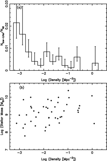
(a) Histogram of the fraction of low-LHα galaxies as a function of all galaxies with the same range of stellar masses in the Whole sample (all galaxies with 0.002 < z < 0.13) at each density. The low-LHα sample is found at the lowest densities and is a higher fraction at the lowest densities. The error bars indicate the 1σ confidence intervals on the binomial population proportions (Cameron 2010). (b) Distribution of the stellar mass with surface density for the lowest-Hα-luminosity galaxies, emphasizing that the lowest-mass systems lie in the least-dense environments.
Fig. 9(b) indicates that the environmental density of the low-Hα-luminosity galaxies is related to their stellar mass. For a given density, the stellar mass is higher in higher density environments. There is only one low-mass galaxy in moderate-density environments [0.1 > densities(galaxy Mpc −2) > 10]. However, there are two higher mass (M∼ 1010 M⊙), low star formation galaxies in the lowest-density environments. The fact that there are no low-mass, low star formation galaxies in high-density environments (density > 10 galaxy Mpc−2) suggests that the only way such low-mass, star-forming galaxies can survive over a Hubble time without being accreted, tidally disrupted or being starved of their gas supply is through residing in the lowest-density environments.
These observations are consistent with measurements of galaxy clustering: the correlation length of the two-point correlation function is observed to increase from less-clustered, low-luminosity blue galaxies (Mr > −19) to more-clustered, high-luminosity blue galaxies (Mr < −21) and even more-clustered red galaxies in the 2dF Galaxy Redshift Survey (Norberg et al. 2002) and SDSS (using photometric redshifts trained on GAMA observations; Christadoulou et al., in preparation).
4 DISCUSSION AND CONCLUSIONS
We have investigated the properties of a sample of 90 of the faintest-Hα-luminosity galaxies from the r-band-selected GAMA survey. We find these galaxies to generally be of low stellar mass, blue and in low-density environments with a range of SFHs. This is the most-distant sample of such low-mass, low star formation systems currently known and with the area of the GAMA survey, the best yet available for probing their environmental dependence.
We have shown that the low-Hα-luminosity galaxies have similar properties to dwarf irregular galaxies in the Local Volume. Local Group galaxies are sufficiently near that their SFHs have been studied in detail through resolved stellar population analysis. In this environment, dwarf galaxies are the most numerous. The Local Group dwarf galaxies appear to have complex, past SFHs, such that whatever star formation is currently occurring, there is always evidence for large intermediate-age populations and for long episodes of low-to-moderate star formation intensity separated by short passive phases (e.g. Smecker-Hane et al. 1996; Skillman et al. 2003; Tolstoy, Hill & Tosi 2009).
We find low-SFR, low-mass systems at higher redshifts than the Local Group/Volume samples yet with similar Hα luminosities and wide ranges of SFHs to the local samples. The continuous distribution of SSFRs we observe suggests that the galaxies cover a range of phases of star formation, some passive, some steady and some bursting. This is consistent with their being higher redshift analogues of local dwarf star-forming systems. As introduced in Section 1, understanding the causes of this range in SFHs is ongoing. Stinson et al. (2007) simulate the collapse of isolated dwarf galaxies and find that star formation in low-mass galaxies can undergo a ‘breathing’ mode where episodes of star formation trigger gas heating leading to galaxies with episodic star formation and significant intermediate-age populations. Quillen & Bland-Hawthorn (2008) show that this ‘breathing’ requires strong, delayed feedback in order to reproduce the observationally estimated episode times. Alternatively, we could have a steeper IMF as recently suggested for galaxies with lower SFRs (e.g. Weidner & Kroupa 2005; Hoversten & Glazebrook 2008; Lee et al. 2009; Meurer et al. 2009; Gunawardhana et al., in preparation).
We find these galaxies to be in low-density environments. That isolation has led to their remaining low mass and star forming, with the lowest-mass galaxies generally found in the lowest-density environments and those in denser environments tending to have higher stellar masses. These observations led to the prediction that at high redshift, when there has been less time for interactions, we would expect to see a higher proportion of low-mass, star-forming systems in dense environments, since they will not have had time to be accreted, tidally stripped or their gas reservoirs rendered ineffective through external processes.
We thank the anonymous referee for comments that improved this paper. SB thanks Phil James, Baerbel Koribalski and Kim-Vy Tran for helpful comments. GAMA is a joint European-Australasian project based around a spectroscopic campaign using the Anglo-Australian Telescope. The GAMA input catalogue is based on data taken from the SDSS and the UKIRT Infrared Deep Sky Survey. Complementary imaging of the GAMA regions is being obtained by a number of independent survey programmes including the GALEX MIS, VST KIDS, VISTA VIKING, WISE, Herschel-ATLAS, GMRT and ASKAP providing UV to radio coverage. GAMA is funded by the STFC (UK), the ARC (Australia), the AAO and the participating institutions. The GAMA website is http://www.gama-survey.org/.
REFERENCES
