


Abstract
We present high spatial resolution optical imaging and polarization observations of the PSR B0540−69.3 and its highly dynamical pulsar wind nebula (PWN) performed with Hubble Space Telescope, and compare them with X-ray data obtained with the Chandra X-ray Observatory. In particular, we have studied the bright region south-west of the pulsar where a bright ‘blob’ is seen in 1999. In a recent paper by De Luca et al. it was argued that the ‘blob’ moves away from the pulsar at high speed. We show that it may instead be a result of local energy deposition around 1999, and that the emission from this then faded away rather than moved outward. Polarization data from 2007 show that the polarization properties show dramatic spatial variations at the 1999 blob position arguing for a local process. Several other positions along the pulsar-‘blob’ orientation show similar changes in polarization, indicating previous recent local energy depositions. In X-rays, the spectrum steepens away from the ‘blob’ position, faster orthogonal to the pulsar-‘blob’ direction than along this axis of orientation. This could indicate that the pulsar-‘blob’ orientation is an axis along where energy in the PWN is mainly injected, and that this is then mediated to the filaments in the PWN by shocks. We highlight this by constructing an [S ii]-to-[O iii]-ratio map, and comparing this to optical continuum and X-ray emission maps. We argue, through modelling, that the high [S ii]/[O iii] ratio is not due to time-dependent photoionization caused by possible rapid X-ray emission variations in the ‘blob’ region. We have also created a multiwavelength energy spectrum for the ‘blob’ position showing that one can, to within 2σ, connect the optical and X-ray emission by a single power law. The slope of that power law (defined from  ) would be αν= 0.74 ± 0.03, which is marginally different from the X-ray spectral slope alone with αν= 0.65 ± 0.03. A single power law for most of the PWN is, however, not be possible. We obtain best power-law fits for the X-ray spectrum if we include ‘extra’ oxygen, in addition to the oxygen column density in the interstellar gas of the Large Magellanic Cloud and the Milky Way. This oxygen is most naturally explained by the oxygen-rich ejecta of the supernova remnant. The oxygen needed likely places the progenitor mass in the 20–25 M⊙ range, i.e. in the upper mass range for progenitors of Type IIP supernovae.
1 INTRODUCTION
PSR B0540−69.3 is a 50.2-ms pulsar in the Large Magellanic Cloud (LMC). A detailed review about the discovery and observations of the pulsar, its wind nebula, as well as the whole supernova remnant (SNR) in all wavelength bands is provided by Williams et al. (2008).
PSR B0540−69.3 is often referred to as the ‘Crab twin’ because it is of similar age (∼1000 yr), it has a similar pulse period and that it has a pulsar wind nebula (PWN) surrounding it, similar to that of the Crab. It has also been suggested that the detailed structures of the two PWNe, as revealed for PSR B0540−69.3 in X-rays (Gotthelf & Wang 2000), are similar, and that PSR B0540−69.3 may have a jet and a torus like the Crab. For further comparison between the two pulsars and their PWNe we refer to Serafimovich et al. (2004).
There are, however, important differences between the two pulsars and their surrounding nebulae. The most obvious is that the supernova ejecta of SNR 0540−69.3 are oxygen rich, although with some hydrogen mixed in (Serafimovich et al. 2005), making it likely that SNR 0540−69.3 and PSR B0540−69.3 (together henceforth referred to as ‘0540’) stem from a Type IIP supernova explosion of a massive (∼20 M⊙) star (Chevalier 2006), whereas the Crab progenitor was a much less massive (8–10 M⊙) star (e.g. Hester 2008). In addition, 0540 has a normal supernova shell of fast ejecta, something which has not yet been fully confirmed to exist around the Crab (see e.g. Tziamtzis et al. 2009). This could mean that the Crab ejecta have much less kinetic energy than the ejecta of 0540 which appears to be normal in that respect.
Closer to the centre, 0540 appears much more asymmetric than the Crab Nebula, with much of the emission coming from a region a few arcseconds south-west of the pulsar. Morse et al. (2006) show that this asymmetric appearance, as well as redward asymmetry in integrated profiles of emission lines (see also Kirshner et al. 1989; Serafimovich et al. 2005), does not signal an overall asymmetry of the PWN as the maximum velocity of emission lines toward and away from us are nearly equal.
Even closer to the centre, a detailed comparison between the PWNe of the two pulsars is more difficult due to the large distance to PSR B0540−69.3 (∼51 kpc; Panagia 2005) as opposed to the 2 ± 0.5 kpc to the Crab (Kaplan et al. 2008 and references there in); the semimajor axis of the torus in the Crab would only subtend ∼1.5 arcsec at the distance of PSR B0540−69.3, and details such as the changing structure of the Crab wisps would have been close to impossible to disentangle even with the Hubble Space Telescope (HST) or ground-based adaptive optics. It therefore comes as no surprise that there is yet no counterpart for PSR B0540−69.3 and its PWN to the detailed synchronized optical and X-ray study of the Crab PWN by Hester et al. (2002). These authors revealed the presence of outward moving equatorial wisps with velocities of ∼0.5 the speed of light. Many time-variable subarcsecond structures exist in the Crab PWN in the optical (Hester et al. 2002), near-infrared (IR; Melatos et al. 2005) and X-rays (Weisskopf, Hester & Tennant 2000; Hester et al. 2002). This is discussed in detail by Hester (2008).
The first indication that also 0540 displays changes in its structure over a relatively short time period was shown by De Luca et al. (2007). They found a 10 yr flux variation (between 1995 and 2005) in the south-west direction where the PWN has its strongest emission and suggested that they had detected a hotspot moving at ∼0.04c. De Luca et al. noted that the hotspot could be similar to a time-varying arc-like feature in the outer Crab Nebula, and that a pulsar jet in 0540 could be directed toward the bright south-west region rather than perpendicular to this, as suggested earlier by Gotthelf & Wang (2000).
In this paper we present a study of the PWN of PSR B0540−69.3 using the same data as De Luca et al. (2007), complemented with all other HST data available for 0540 as well. In particular, we have included recent HST polarization data from 2007. We also include all available X-ray data of 0540.
The paper is organized as follows: in Section 2 we describe and discuss the observations, in Section 3 the analysis and results and in Section 4 we conclude with a discussion.
2 OBSERVATIONS
2.1 HST observations and data analysis
The pulsar field was observed with HST/Wide Field Planetary Camera 2 (WFPC2) in 2005 (Program ID 10601) using the two broad-band filters F547M and F555W (see Table 1). As opposed to earlier HST/WFPC2 observations of PSR B0540−69.3 we used a dithering procedure for all images to better avoid cosmic ray (CR) contamination. PSR B0540−69.3 and its PWN were exposed on the PC chip, and the observations were made in a two-gyro mode. The CCD amplification, i.e. gain was 7.12 and readout noise = 5.24. The reason for choosing the continuum filter F547M was that the main goals of the observations were to study the proper motion of the pulsar, as well as the spectrum of the pulsar and the PWN. In earlier observations the pulsar and PWN were mainly studied in filters largely contaminated with line emission from filaments in 0540. Continuum filters like F547M avoid this contamination. The 2005 data have been discussed by De Luca et al. (2007), and an upper limit to the proper motion of the pulsar was estimated, as well as identifying the apparent displacement of a feature in the PWN. We discuss this further here, as well as use the data for spectral studies of the PWN.
HST/WFPC2 optical observations of the PSR B0540−69.3 field used in our study.
| Date | Total | Filter | Proposal | Comments | ||
| exposurea | Name | PHOTPLAMb | PHOTBWc | ID | ||
| 1992 November 17d | 2 × 400 | F547M | 5483.9 | 205.5 | 4244 | Continuum |
| 1995 October 19 | 2 × 300 | F555W | 5442.9 | 522.2 | 6120 | Overlaps with [O iii]λ5007 |
| 1999 October 17 | 2 × 300 | F336W | 3359.5 | 204.5 | 7340 | Continuum |
| 1999 October 17 | 8 × 1300 | F502N | 5013.3 | 48.3 | ⋅⋅⋅ | Centred on [O iii]λ5007 |
| 1999 October 17 | 2 × 400 | F547M | 5483.9 | 205.5 | ⋅⋅⋅ | Continuum |
| 1999 October 17 | 6 × 1300 | F673N | 6732.3 | 30.7 | ⋅⋅⋅ | Centred on [S ii]λλ6716, 6731 |
| 1999 October 17 | 2 × 200 | F791W | 7872.5 | 519.8 | ⋅⋅⋅ | Continuum |
| 2005 November 15e | 4 × 260 | F547M | 5483.9 | 205.5 | 10601 | Continuum |
| 2005 November 15e | 3 × 160 | F555W | 5442.9 | 522.2 | ⋅⋅⋅ | Overlaps with [O iii]λ5007 |
| 2007 June 21 | 3 × 260 | F336W | 3359.5 | 204.5 | 10900 | Continuum |
| 2007 June 21 | 3 × 260 | F450W | 4557.3 | 404.2 | ⋅⋅⋅ | Continuum |
| 2007 June 21 | 3 × 100 | F555W | 5442.9 | 522.2 | ⋅⋅⋅ | Overlaps with [O iii]λ5007 |
| 2007 June 21 | 3 × 140 | F675W | 6717.7 | 368.3 | ⋅⋅⋅ | Overlaps with [S ii]λλ6716, 6731 |
| 2007 June 21 | 3 × 200 | F814W | 7995.9 | 646.1 | ⋅⋅⋅ | Continuum |
a Total exposure is given in number of images times the exposure time of individual images in seconds.
b Pivot wavelength of the filter band measured in Å.
c Width of the filter band measured in Å.
d The 1992 observations were obtained with HST/WFPC instead of HST/WFPC2.
e Our observations.
To study time variability of the PWN we also used available archival HST/WFPC and WFPC2 data obtained from 1992 to 2007 (Table 1). There are three different storage sites of HST observations, namely the MAST,1 CADC2 and ST-ECF.3 All three archives use slightly different calibration plans, or pipeline reductions of raw data. We found that the pipeline reduced data of the same WFPC2 observations from these archives give different results for the photometry of PSR B0540−69.3 and its neighbourhood. In previous work (Serafimovich et al. 2004) we did not resort to pipeline reductions, but made careful manual reductions of the raw data. Using photometric results from that work we found that only the data from the MAST archive with their recent pipeline calibration plan can reproduce our previous photometry. To avoid systematic differences due to pipeline effects in our analysis we therefore used the data only from the MAST archive with the most recent calibration plan for all epochs of HST/WFPC2 observations listed in Table 1.
All data were reduced using iraf in combination with stsdas and dither4 packages. Pre-calibrated data include references to the latest distortion correction files available at the STScI.5 Using STScI recommendations6 we used these files together with the multidrizzle package for each individual image independently. CR cleaning and combining of the images were excluded at this step. This exclusion was essential for the 1995 and 1999 epochs. These observations were performed without dithering in between exposures, and after cleaning and combining, multidrizzle introduced extra noise in the pixel distribution which led to an overestimate of faint source fluxes. The overestimate for F547M in the 1999 epoch was found to be a factor of around 2. After multidrizzle, the individual images were converted from the unit of electrons per second to counts using the iraf/imgtools/imcalc utility, e.g. (image × exposure)/gain. Final image combining was performed using the standard iraf imcombine utility with CR rejection by setting reject = crreject.
The data obtained in 2005, and later, clearly show that the charge transfer efficiency (CTE) effect (Riess 2000) on HST/WFPC2 images was getting worse with time (see Fig. 1). The CTE effect is very complicated to compensate for as it is time, position and flux dependent, i.e. it is unique for every particular point source and almost unknown for extended objects. In order to more reliably study the structure of the PWN, we used the multiscale filtering method described in Sections 2.5 and 3.1.
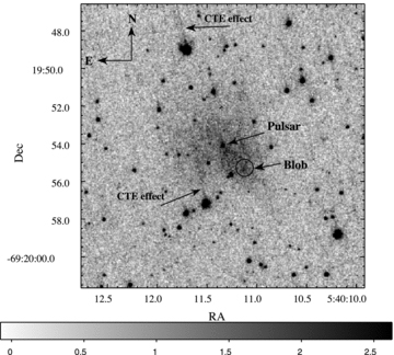
A 15 × 15 arcsec2 image of the field around PSR B0540−69.3 obtained in the F547M band with HST/WFPC2 in 2005 (Table 1). The pulsar was exposed on the PC chip and its position is marked by an arrow. The diffuse emission surrounding the pulsar is the PWN. A highly variable area or ‘blob’ is marked by a circle and an arrow. Two typical traces of the CTE effect are marked by arrows (see text for more details).
2.2 Chandra X-ray observations
To compare the structure of the PWN in the optical and X-rays, we utilized the Chandra archival data listed in Table 2. The High-Resolution Camera (HRC-I) observations of 0540 were obtained as part of the instrument calibration plan in 1999 and 2000, only a few months before and after the HST 1999 observations described in Table 1. They contain very limited spectral information, but provide the best spatial resolution (pixel size 0.132 arcsec) in X-rays, and are therefore the most useful for the study of the PWN morphology. The Advanced CCD Imaging Spectrometer (ACIS-S) observations (PI S. Park) have lower spatial resolution (pixel size 0.492 arcsec), but provide better spectral information. The ACIS-S observations started only 3 months after our HST observations in 2005, and are useful for an optical/X-ray comparison, assuming the PWN structure did not change substantially in 3 months. Another advantage of these observations is that the 1/4 ACIS-S subarray mode was used7 and the data are much less contaminated by the CCD pileup effects from the high count rate of the pulsar in the centre of the PWN, as opposed to previous ACIS observations, e.g. the data obtained in 1999 November 23 (Petre et al. 2007; Obs ID 119, exposure 28.16 ks). For the latter, significant pileup precludes a reliable spatial and spectral analysis of the central PWN regions. The HRC-I data are not affected by the pileup.
Chandra X-ray observations of the PSR B0540−69.3 field used in our study.
| Date | Exposure (ks) | Instrument | ObsID |
| 1999 August 31 | 17.79 | HRC-I | 132 |
| 2000 June 21 | 10.04 | HRC-I | 1735 |
| 2000 June 21 | 10.04 | HRC-I | 1736 |
| 2000 June 22 | 10.07 | HRC-I | 1741 |
| 2006 February 15 | 40.36 | ACIS-S | 5549 |
| 2006 February 16 | 39.98 | ACIS-S | 7270 |
| 2006 February 18 | 38.56 | ACIS-S | 7271 |
2.3 HST/WFPC2 polarization observations
To better understand the highly variable structure in the south-western part of the 0540 PWN we utilized HST/WFPC2 archival polarization data.
PSR B0540−69.3 and its wind nebula were observed in polarized light with HST/WFPC2 in 2007 (Program ID 10900) using the broad-band filter F606W in combination with the POLQ polarizer (see Table 3). The field was exposed only on the PC chip during all sets of observations using different rotations of the HST to reproduce the required polarization angle (see column 4 in Table 3). This gives the presently highest spatial resolution available for polarization observations, i.e. 0.0455 arcsec pixel−1. Unfortunately, the pulsar and its nebula were placed mainly in the vignetted area of the PC chip. Since the part of the nebula was never more than 4 arcsec into the bad area, the loss of light was not so big. However, this made calibrations slightly more cumbersome.
HST/WFPC2 polarization observations of the PSR B0540−69.3 field used in our study.
| Date | Total exposurea | Mode of obs. | Pol. angle (°) | Proposal ID |
| 2007 November 5 | 600 × 3 | F606W+POLQ | 0 | 10900 |
| 2007 September 25 | 600 × 3 | F606W+POLQ | 45 | 10900 |
| 2007 July 26 | 600 × 3 | F606W+POLQ | 90 | 10900 |
| 2007 June 21 | 600 × 3 | F606W+POLQ | 135 | 10900 |
| Date | Total exposurea | Mode of obs. | Pol. angle (°) | Proposal ID |
| 2007 November 5 | 600 × 3 | F606W+POLQ | 0 | 10900 |
| 2007 September 25 | 600 × 3 | F606W+POLQ | 45 | 10900 |
| 2007 July 26 | 600 × 3 | F606W+POLQ | 90 | 10900 |
| 2007 June 21 | 600 × 3 | F606W+POLQ | 135 | 10900 |
a The total exposure is given in number of images times the exposure time of individual images in seconds.
Because of the long exposures (600 s) each frame exhibits thousands of CR hits. Most of these we removed by temporal median filtering of the three images, and the remaining hits are removed by la-cosmic which is included in the idl software. The images were taken at the roll angles 0°, 45°, 90° and 135°, and to align the images three of them must be rotated and shifted. The de-rotation of 45° and 135° requires interpolation, and so do the shifts. We used a cubic spline interpolation scheme and even though we succeed in overlapping the images to an accuracy of 10 mas, it is clear that the resulting point spread function (PSF) for point sources may be affected. This means that we must be careful in our interpretation of polarization close to point sources. On the other hand, the extended emission, which is the focus of the present investigation, is not affected by the interpolations.
2.4 Astrometric referencing
Astrometric referencing of the HST/WFPC2 images was performed based on the positions of the astrometric standards selected from the USNO-B1 astrometric catalogue.8 A dozen of the USNO-B1 reference objects can be identified within the PC2 chip field-of-view (FOV). Their 1σ coordinate uncertainties vary between 50 and 900 mas with an rms value of about 330 mas. Pixel coordinates of the standards were derived using of the iraf task imcenter with an accuracy of 0.05–0.1 PC2 pixel size (0.042 arcsec). The iraf tasks ccmap/cctran were applied for the astrometric transformation of the images. We consequently discarded standards which are either oversaturated or have relatively large catalogue and image positional uncertainties. As a result, only seven stars were selected for the final astrometric fit. Formal rms uncertainties of the fit were best for the F814W filter ΔRA ≲ 0.32 arcsec and ΔDec. ≲ 0.43 arcsec, and the fit residuals are ≲0.6 arcsec, which is compatible with the maximum catalogue position uncertainty of the finally selected standards (0.33 arcsec). The rest PC2 images were referenced to the F814W image with the accuracy better than 0.1 (0.004 arcsec) of the PC2 pixel size using several unsaturated stars from the PWN neighbourhood. Finally, the first F547M images obtained in 1992 with the WFPC at a worse spatial resolution (pixel size 0.1 arcsec) were aligned to the WFPC2 images with the accuracy of about 0.02 arcsec.
Inspection of the Chandra/HRC and ACIS images obtained in 2000 and 2006 showed that within a nominal Chandra pointing accuracy of ≲0.5 arcsec they are in a perfect agreement with the referenced optical images both by the pulsar coordinates and the orientation of the PWN. For the HRC observations of 1999 we found a large formal systematic shift of the pulsar coordinates form their correct values by 22.1 and −84.02 pixels of the CCD x and y coordinates, respectively. After the correction by this shift the object position and the PWN orientation are in agreement with those at the other X-ray and optical images obtained at different epochs.
All this allows us to compare the optical and X-ray structures of the PWN at a subarcsecond accuracy level. To get deeper X-ray images of 2000 and 2006 the respective multiple data sets were combined making use of the merge-all v3.6 script of the ciao tool.
2.5 Wavelet filtering of the HST/WFPC2 images
2.5.1 Wavelet filtering
 and the smooth version of the image Cp.
2.5.2 Wavelet filtering to study the optical variability of the PWN
To study the optical variability of the PWN, we have to focus on the diffuse emission surrounding the pulsar. For this purpose, we have used a detection method to extract off the pulsar and other stars contained in the field. The detection method requires a multiscale vision model (MVM) defined in Bijaoui & Rué (1995) and Starck & Murtagh (2006), based on the ‘à trous’ wavelet transform described previously. The MVM describes an object as a set of structures at different scales and a structure is a set of significant connected wavelet coefficients at the same scale j. Assuming a Gaussian noise, the definition of a significant wavelet coefficient is given by expression (3). A prior can be introduced to change slightly this definition. For instance, in order to extract off the pulsar and other stars, we can consider there is no interesting object larger than a given size. Then, we can force to 0, the wavelet coefficients larger than this size. Having detected all the interesting objects in the field (e.g. pulsar and stars), they can be extracted by subtraction (see Starck & Murtagh 2006 for more details). The remaining signal is the diffuse emission coming from the PWN. This is the emission we aim to study.
3 RESULTS
3.1 CTE effect and proper motion of PSR B0540−69.3
Modern techniques like wavelet filtering of images helps to bring out faint features and filters off traces of CTE. In order to investigate the importance of CTE effect on coordinate measurements or flux measurements we performed the following test on filtered and non-filtered images. We selected several background stars close to PSR B0540−69.3, including stars projected on the PWN. We used filtered and non-filtered F555W images for the 1995 and 2005 epochs. We measured coordinates on both sets of images using iraf imcentroid. Filtered and non-filtered images show no significant difference in accuracy within the image. A representative result obtained on filtered images is shown in Fig. 2, where we plot the distance between the pulsar and 13 stars with similar brightness as the filaments in the PWN, i.e. between magnitude 21 and 23, versus the positional uncertainty of the stars. In general, fainter stars produce higher residuals, but the numbers are low, and there is no clear trend that the 2005 image gives higher residuals due to the CTE effect. We can therefore conclude that the CTE effect is unimportant for measurements of point sources, since the core of a star defines the position, which is unaffected by the CTE tail.
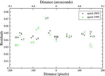
Coordinate measurements of 13 stars in wavelet filtered F555W images for the 1995 and 2005 epochs (see text for further details).
Main uncertainties arise when one aligns images from different epochs and sets of observations. The mean accuracy for this is about 0.1 of a WFPC2/PC chip pixel (or 0.005 arcsec) (see Section 2.4). At this accuracy level we do not find any significant displacement of the pulsar position for the considered time base of 1999–2007. This is in agreement with the constraints on the pulsar proper motion recently reported by De Luca et al. (2007) using HST data between 1995 and 2005.
The situation becomes very different when we try to measure fluxes of point sources, since part of the flux is in the CTE tail. We have tested different aperture sizes and find that the most optimal size is 10 WFPC2/PC chip pixels, or ∼0.5 arcsec. This aperture encapsulates a star of magnitude 21–23 and its CTE tail. This aperture was chosen for most of our photometric measurements.
3.2 Optical photometry
To study spectral properties of the PWN we performed detailed photometry of selected areas in all optical continuum filters for 1999 and 2007.
We selected several areas in the PWN to perform photometry using the optical broad-band filters. The aperture radius was 10 HST pixels, and the aperture was centred on the maximum of flux of the ‘blob’. Following De Luca et al. (2007), we therefore centred on different areas for the 1999 and 2005 images. However, for the 2007 epoch, there is no obvious dominant feature, and the aperture centre corresponds to the assumed position of the ‘blob’, had it continued to move with 0.04 times the speed of light as suggested by De Luca et al. (2007). An aperture of the same size was also placed on the apposite side of the pulsar position along the major symmetry axis of the PWN and at the same distance away from the pulsar as the ‘blob’. We call this the ‘antiblob’ aperture (see Fig. 3).
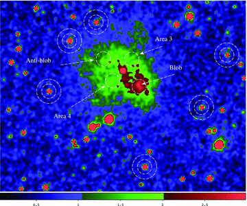
PSR B0540−69.3 and its PWN as observed with HST/F547M in 1999. The white circular apertures show the ‘blob’ position in 1999, the ‘antiblob’, ‘Area 3’ and ‘Area 4’, as well as six references stars (see text for more details). Some stars projected on the PWN were subtracted off.
We also selected two 10 HST pixels apertures along the minor symmetry axis of the PWN, symmetrically on both sides of the pulsar position, and name these ‘Area 3’ and ‘Area 4’. Thanks to the high spatial resolution of the HST/WFPC2/PC chip (0.0455 arcsec pixel−1), we were able to measure the optical fluxes in these areas. For the optical background estimate for these areas we used annulus apertures of 6 HST pixels around six selected stars (see Fig. 3).
Photometry for all selected apertures was performed using iraf/digiphot/phot. The results are presented in Table 4 and Fig. 4. ‘Area 3’ and ‘Area 4’ show slight brightening from epoch 1999 to 2007, but with similar spectral index, α, defined as Fν∝ν−α. The area ‘antiblob’ does not show any change within errors in flux and spectral index between the two epochs.
Results of optical spectral fits for several regions of the 0540 pulsar+PWN system. Columns 6 and 7 are the measured and dereddened fluxes with E(B−V) = 0.20 (AV = 0.62), respectively.
| Epoch | Source | Band | Log (flux) | Power law | ||||
| Region | Area | Name | Log(ν) | Observed | Dereddened | ανa | Norm. const.b | |
| (arcsec2) | (Hz) | (μJy) | (μJy) | (μJy) | ||||
| 1999 | Blob | 14.3 | F791W | 14.581(15) | 1.343(18) | 1.496(18) | 1.35(+27−22) | |
| ⋅⋅⋅ | ⋅⋅⋅ | ⋅⋅⋅ | F547M | 14.738(8) | 1.026(20) | 1.275(20) | ⋅⋅⋅ | 1.28(+3−3)c |
| ⋅⋅⋅ | ⋅⋅⋅ | ⋅⋅⋅ | F336W | 14.950(13) | 0.584(82) | 0.989(82) | ⋅⋅⋅ | |
| 2007 | Blob | 14.3 | F814W | 14.574(18) | 1.255(20) | 1.403(20) | 1.06(+18−16)c | |
| ⋅⋅⋅ | ⋅⋅⋅ | ⋅⋅⋅ | F675W | 14.649(12) | 1.160(22) | 1.357(22) | ⋅⋅⋅ | |
| ⋅⋅⋅ | ⋅⋅⋅ | ⋅⋅⋅ | F555W | 14.741(21) | 0.974(26) | 1.224(26) | ⋅⋅⋅ | 1.24(+2−2) |
| ⋅⋅⋅ | ⋅⋅⋅ | ⋅⋅⋅ | F450W | 14.818(20) | 0.837(26) | 1.152(26) | ⋅⋅⋅ | |
| ⋅⋅⋅ | ⋅⋅⋅ | ⋅⋅⋅ | F336W | 14.950(13) | −0.006 | 0.398d | ||
| ⋅⋅⋅ | ⋅⋅⋅ | ⋅⋅⋅ | F336W | 14.950(13) | 0.188(72) | 0.593(72)e | ||
| ⋅⋅⋅ | ⋅⋅⋅ | ⋅⋅⋅ | F336W | 14.950(13) | 0.510(50) | 0.915(50)f | ||
| 1999 | Antiblob | 14.3 | F791W | 14.581(15) | 1.012(28) | 1.164(28) | 0.90(+35−27) | |
| ⋅⋅⋅ | ⋅⋅⋅ | ⋅⋅⋅ | F547M | 14.738(8) | 0.707(32) | 0.955(32) | ⋅⋅⋅ | 1.00(+3−4)c |
| ⋅⋅⋅ | ⋅⋅⋅ | ⋅⋅⋅ | F336W | 14.950(13) | 0.408(108) | 0.813(108) | ⋅⋅⋅ | |
| 2007 | Antiblob | 14.3 | F814W | 14.574(18) | 1.036(26) | 1.184(26) | 1.00(+33−25) | |
| ⋅⋅⋅ | ⋅⋅⋅ | ⋅⋅⋅ | F675W | 14.649(12) | 0.976(26) | 1.173(26) | ||
| ⋅⋅⋅ | ⋅⋅⋅ | ⋅⋅⋅ | F555W | 14.741(21) | 0.742(38) | 0.992(38) | ||
| ⋅⋅⋅ | ⋅⋅⋅ | ⋅⋅⋅ | F450W | 14.818(20) | 0.641(36) | 0.956(36) | ⋅⋅⋅ | 0.94(+5−6) |
| ⋅⋅⋅ | ⋅⋅⋅ | ⋅⋅⋅ | F336W | 14.950(13) | 0.382(118) | 0.787(118) | ⋅⋅⋅ | |
| 1999 | Area 3 | 14.3 | F791W | 14.581(15) | 1.071(32) | 1.224(32) | 1.30(+44−33) | |
| ⋅⋅⋅ | ⋅⋅⋅ | ⋅⋅⋅ | F547M | 14.738(8) | 0.763(34) | 1.012(34) | ⋅⋅⋅ | 1.02(+4−5)c |
| ⋅⋅⋅ | ⋅⋅⋅ | ⋅⋅⋅ | F336W | 14.950(13) | 0.318(132) | 0.723(132) | ⋅⋅⋅ | |
| 2007 | Area 3 | 14.3 | F814W | 14.574(18) | 1.086(28) | 1.234(28) | 1.32(+42−31) | |
| ⋅⋅⋅ | ⋅⋅⋅ | ⋅⋅⋅ | F675W | 14.649(12) | 1.035(28) | 1.232(28) | ||
| ⋅⋅⋅ | ⋅⋅⋅ | ⋅⋅⋅ | F555W | 14.741(21) | 0.799(36) | 1.049(36) | ||
| ⋅⋅⋅ | ⋅⋅⋅ | ⋅⋅⋅ | F450W | 14.818(20) | 0.753(30) | 1.067(30) | ⋅⋅⋅ | 0.95(+5−8) |
| ⋅⋅⋅ | ⋅⋅⋅ | ⋅⋅⋅ | F336W | 14.950(13) | 0.276(146) | 0.681(146) | ⋅⋅⋅ | |
| 1999 | Area 4 | 14.3 | F791W | 14.581(15) | 1.074(26) | 1.226(26) | 1.00(+35−28) | |
| ⋅⋅⋅ | ⋅⋅⋅ | ⋅⋅⋅ | F547M | 14.738(8) | 0.796(28) | 1.045(28) | ⋅⋅⋅ | 1.06(+3−3) |
| ⋅⋅⋅ | ⋅⋅⋅ | ⋅⋅⋅ | F336W | 14.950(13) | 0.436(108) | 0.841(108) | ⋅⋅⋅ | |
| 2007 | Area 4 | 14.3 | F814W | 14.574(18) | 1.098(24) | 1.246(24) | 0.86(+26−21) | |
| ⋅⋅⋅ | ⋅⋅⋅ | ⋅⋅⋅ | F675W | 14.649(12) | 0.951(30) | 1.146(30) | ||
| ⋅⋅⋅ | ⋅⋅⋅ | ⋅⋅⋅ | F555W | 14.741(21) | 0.746(40) | 0.996(40) | ||
| ⋅⋅⋅ | ⋅⋅⋅ | ⋅⋅⋅ | F450W | 14.818(20) | 0.696(34) | 1.010(34) | ⋅⋅⋅ | 1.03(+4−5) |
| ⋅⋅⋅ | ⋅⋅⋅ | ⋅⋅⋅ | F336W | 14.950(13) | 0.515(94) | 0.920(94) | ⋅⋅⋅ | |
a Dots in the column show which filters were used for power-law fitting.
b The row shows which pivot frequency was used for the normalization.
c The power law was fitted without the F336W data.
d An upper limit. The aperture was placed on the estimated blob position in 2007.
e The aperture was placed on the estimated blob position in 2005.
f The aperture was placed on the estimated blob position in 1999.
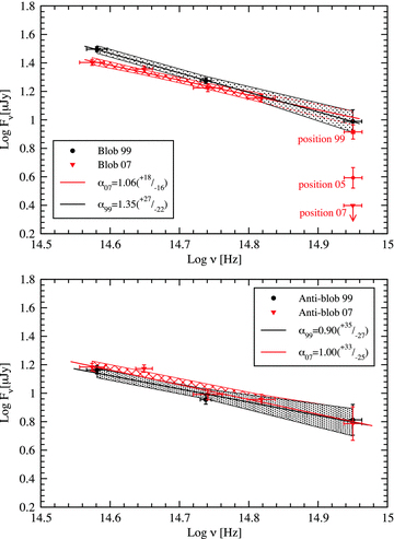
Broad-band optical spectra for the selected areas shown in Fig. 3. In the top panel we show the ‘blob’ spectrum in red for 2007 and black for 1999. For the 2007 ‘blob’ spectrum we have applied a 0.4-arcsec shift for the aperture, corresponding to a 0.04c motion of the ‘blob’, as suggested by De Luca et al. (2007). For the spectral fit of this spectrum, we have omitted the F336W data (see text). The sensitivity of the F336W to where the aperture is placed is shown in the plot. Data in other bands are less sensitive (see Section 3.6). For the ‘antiblob’ we did not apply any shift in aperture position between 1999 and 2007.
The most interesting behaviour is displayed by the ‘blob’. First of all, the flux of the ‘blob’ became significantly lower in 2007 compare to 1999. On other hand, the spectral index became shallower in 2007 (see Table 4), corresponding to a harder electron spectrum. There are two possible hypotheses: either the ‘blob’ moves with ∼0.04c times the speed of light, as suggested by De Luca et al. (2007) when they compared 1995, 1999 and 2005 images, or it fades away. We studied both these hypotheses.
The ‘blob’ was in its brightest phase in 1999. The aperture was centred on the maximum of the flux within the area. In later epochs we placed the aperture on expected positions taking into account an assumed speed of 0.04c. For the F336W image in 2007 the expected position of the ‘blob’ is outside the visible PWN. Since the PWN has quite steep power law, and since the extinction is higher in the blue, we only have an upper limit on the flux of the ‘blob’ in the F336W band (see Table 4 and Fig. 4). This spectral point was not included in calculations of the power law for the ‘blob’ in 2007. All power law calculations were done using the algorithm described in Serafimovich et al. (2004). Fluxes in F555W and F675W are contaminated by emission lines of [O iii]λλ4959, 5007 (Morse et al. (2006)) and [S ii]λλ6716, 6731, respectively, which could add some systematic error to the continuum flux for those data entries in Table 4 and Fig. 4.
3.3 Polarization of the PWN of PSR B0540−69.3
First optical polarization measurements for 0540 were performed by Chanan & Helfand (1990) using the Cerro Tololo Inter-American Observatory (CTIO) 4-m telescope. Chanan & Helfand found a linear optical (V band) polarization, integrated over the PWN, which was P = 5.6 ± 1.0 per cent, oriented at a position angle (eastward from north) 79°± 5°. The time integrated observations with a spatial resolution of 0.6 arcsec pixel−1 did not allow them to detect any fine details. The first polarimetric phase-resolved observations of the PSR B0540−69.3 reported by Middleditch, Pennypacker & Burns (1987) gave only an upper limit to the polarization.
A few years later, time integrated optical polarization observations were performed by Wagner & Seifert (2000) using the 8-m Very Large Telescope (VLT). Wagner & Seifert found up to 20 per cent of linear polarization at the rim of the diffuse nebulosity, and 5 per cent for the pulsar. In this case, the spatial resolution was 0.2 arcsec, but the seeing conditions (from 0.4 to 1 arcsec) could not bring out any detailed structures.
Polarization of the 0540 PWN has also been studied at 3.5, 6 and 20 cm in the radio, taking into account the Faraday rotation effect (Dickel et al. 2002). Dickel et al. obtained a total fractional polarization of 20 per cent at 3.5 cm, 8 per cent at 6 cm and 4.5 per cent at 20 cm. They conclude that this large change in polarization with wavelength might be a result of high depolarization. The orientation is consistent with the optical value as reported by Chanan & Helfand (1990). Dickel et al. (2002) noted that there is a gradient in rotation measure, which depends on magnetic field strength and electron number density, from north-east to south-west.
The latest optical polarization observations of 0540 (see description in Section 2.3) are compatible with earlier results, but bring out many new interesting details due to the very high spatial resolution of HST/WFPC2. Fig. 5 shows a continuum intensity image of the PWN with overlaid linear polarization vectors. Polarization vectors represent the electric field vector, E, which is perpendicular to the magnetic field. The length of the vectors shows the degree of polarization. The overall picture is quite complicated. As can be seen in Fig. 5, the outer parts of the PWN have high polarization, on the order of 30–40 per cent. A similar behaviour has been seen for the Crab PWN (see Hester 2008 and references therein).
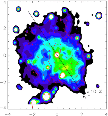
Continuum intensity (Stokes I) image at 602 nm of the PWN centred on PSR B0540−69.3 with overlaid linear polarization vectors. The size of the vector is degree of polarization in per cents, while orientation of a vector is the position angle of linear polarization. A horizontal tick mark to the lower right shows 10 per cent degree of polarization. The major axis of the nebula, used for Fig. 7, is marked by a solid line going from north-east to south-west, cutting across the pulsar and the ‘blob’ seen here in yellow. The x and y axes show distances north and west of the pulsar in arcseconds.
The pulsar itself has low polarization, i.e. 5 ± 2 per cent. This is consistent with earlier observations, but is in stark contrast to recently reported results of 16 ± 4 per cent by Mignani et al. (2010), using the same data set as we have used. The difference might originate from the difficulties of separating the pulsar from the nebula, which has high polarization. Another source of the different results might be different data reduction procedures (see Section 2.3), in particular the correction for the instrumental polarization.
The brightest parts of the 0540 PWN in optical continuum are also in general the brightest in polarized light. It is highlighted by the correlation in Fig. 6. This is perhaps not so surprising since the nebula emits synchrotron radiation, which can be highly polarized for ordered magnetic fields. As can be seen in Fig. 5, the vector E is perpendicular to, or at least not aligned with the major symmetry axis in the bright green area. Such flow of charged particles, which could be a jet, may excite ejecta filaments and perhaps cause shock activity in the ‘blob’ area (see Section 4.1). The possibility of a jet along the major axis was briefly mentioned by De Luca et al. (2007). However, what is most surprising in Fig. 6 is how weak the correlation is between optical continuum flux and polarized flux. The figure suggests that there is a general smooth polarized flux in the nebula, on top of which there is more spatial variation in the non-polarized flux. The ‘blob’ area stands out as the region with the highest intensity and smallest error bar in polarized flux. Its polarized flux is slightly lower than other bright areas in the PWN, which may suggest less ordered magnetic field in the ‘blob region’.
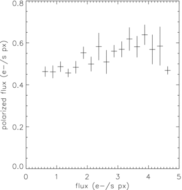
Polarized flux (Stokes  ) as a function of optical brightness (Stokes I) over the whole PWN in 2007. Note the weak correlation between polarized flux and intensity. The ‘blob’ area is the region with the highest intensity and smallest error bar in polarized flux.
To explore the polarization properties more in detail along the major symmetry axis, we have studied a 1-arcsec-wide slice, centred on and along the major axis. We will later also use a similar slice for X-ray projections and the non-polarized optical data (see below). Fig. 7 shows flux (black), polarized flux (red) and polarization angle (blue). We also show the position angle of the major axis (blue horizontal line). The largest maximum (around 1.2 arcsec) to the right of pulsar is close to the ‘blob’ position in 1999. We can see that the polarized flux jumps by a factor of ∼3 at this position, with a small shift by ∼0.1 arcsec further away from the pulsar for the polarized flux compared to the continuum intensity. At the same time, the polarization angle swings ∼60° going from the inside of the blob to where the polarized flux peaks. The alignment of the E field and the major axis is ∼20° at the position of peak intensity. This is close to what is observed for presumed shocks in extragalactic jets, where the E vector abruptly swings from perpendicular to the jet, to parallel, at jet knots. We see a similar behaviour on the opposite side of the pulsar at about 1.0 arcsec, although the structure is less clear. That the position angle of the polarization vector changes just before the polarized flux reaches a maximum at the ‘blob’ position, and perhaps close to the ‘antiblob’ position, could point to shock activity (present or past) in those regions.
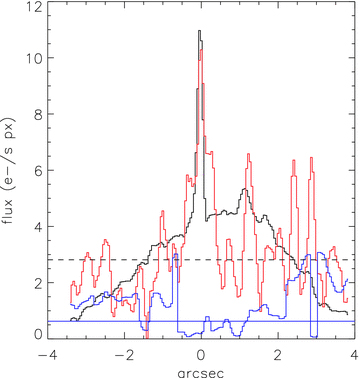
Flux (Stokes I), polarized flux (Stokes  ) and polarization angle along the major symmetry axis in 2007 (shown in Fig. 5). The black curve is the flux, the red curve is the polarized flux multiplied by 10 and the dashed line is the 3σ confidence level for the polarized flux. The blue horizontal straight line is the position angle of the major axis in Fig. 5, and the blue curve indicates the polarization angle, θ, in radians relative to north (i.e. the position angle of the E vector). Note how θ spans its full 0–π range. The pulsar stands out as a peak in the flux and polarized flux at 0 arcsec, and the peaks in flux and polarized flux at ∼1.2 arcsec correspond roughly to the ‘blob’ position in the 1999 and 2000 optical continuum and X-ray images, respectively (see Figs 8 and 9).
We can also see two maxima in polarized flux well above 3σ on the same side as the ‘blob’, but at ∼2.3 and ∼2.8 arcsec away from the pulsar. For the one at ∼2.3 arcsec, the position angle swings away from being parallel to the symmetry axis to being perpendicular, and at ∼2.8 arcsec the electric vector is parallel to that between the pulsar and the ‘blob’. Note that the polarized flux is almost as bright in those regions as it is at the ‘blob’ position. We see a weak, but similar trend, also on the opposite side of the pulsar, outside the ‘antiblob’ position.
3.4 X-ray counterpart of the ‘blob’
To investigate how the X-ray emission correlates with the optical and polarization data, we carefully aligned the optical and X-ray images as described in Section 2.4, and extracted intensity profiles along major and minor PWN symmetry axes. We chose 0.8 × 10 arcsec2 slit size to cover the ‘blob’ in the best way, taking into account the resolution of different instruments.
Figs 8 and 9 show an optical image in F547M taken in 1999 October and an X-ray image in HRC-I taken in 2000 June, with their respective profiles. The position of the ‘blob’ is marked by vertical dotted line at the bottom panel in Fig. 8 (see also the left-hand panel of Fig. 11 for the 2006 Chandra/ACIS data). The spatial profile clearly shows a maximum of flux from that area. As can be seen in the bottom panel in Fig. 9 the same optical coordinates correspond to a maximum of flux from the ‘blob’ area also in X-rays. This clearly shows that the enhanced X-ray and optical radiation come from the same area.
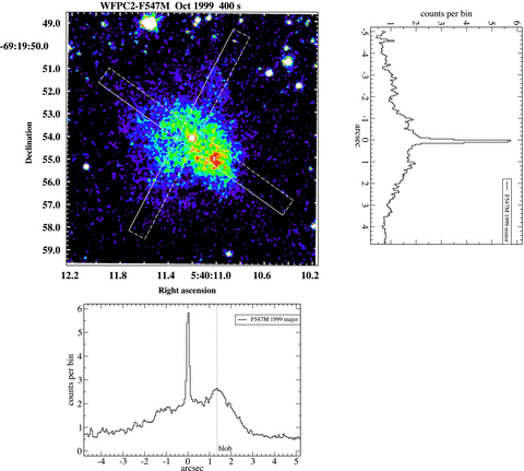
Top left: 11 × 11 arcsec2 optical image of the 0540 pulsar+PWN system taken in 1999 October with the HST/WFPC2 in the F547M band. Positions of two slices with the sizes of 0.8 × 10 arcsec2 are marked by white lines. They were used for the extraction of the one-dimensional spatial profiles along the minor (north-west–south-east) and major (north-east–south-west) axes of the system shown in the top-right and bottom panels, respectively. Coordinate origins of the spatial axis in the profile plots coincide with the position of the pulsar visible as a bright point source near the PWN centre. The position of the bright PWN ‘blob’ seen south-west of the pulsar is marked by a vertical dotted line at the bottom panel.
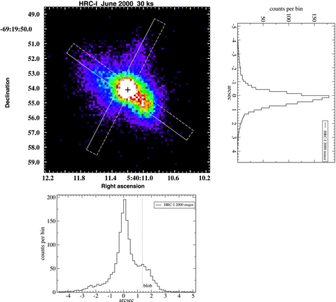
Same as in Fig. 8. but for the X-ray data taken in 2000 June with Chandra/HRC-I in the 0.2–10 keV band. The slice positions and sizes are the same as in the optical image. The cross in the top-left panel marks the optical position of the pulsar, while the vertical line at the bottom panel shows the position of the PWN ‘blob’ in the optical in 1999 October (see also the left-hand panel of Fig. 11 for the 2006 Chandra/ACIS data). As seen, despite the half-year difference between the optical and X-ray observations, a likely X-ray counterpart of the optical ‘blob’ can be seen at the same place as in the optical range.
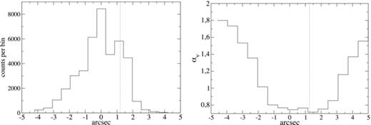
Left: ACIS-S X-ray intensity along the same major axis slice as in Fig 9. Right: index spatial profile along the same slice. Coordinate origins of the spatial axes coincide with the pulsar position, and the vertical dotted line marks the position of the blob. South-west is to the right of the plots. The intensity and index maps were smoothed with a one ACIS pixel Gaussian kernel before the sampling along the slice was made.
We have performed the same investigation for the second epoch for which we have near-coincident optical and X-ray data, i.e. for 2005/2006. The optical emission shows a change in morphology of the ‘blob’ as discussed later in the paper, while the X-ray emission does not show any change in morphology to within the spatial resolution. Note that the worse spatial resolution of Chandra/ACIS compared to Chandra/HRC.
3.5 ACIS-S X-ray spectroscopy
Kaaret et al. (2001) were the first to attempt a study of the X-ray spectral structure of the 0540 PWN. They used the observation carried out on 1999 August 26 with the ACIS-I in a continuous-clocking (CC) mode. A one-dimensional image oriented approximately along the major axis of the nebula including the pulsar was analysed. Spectra extracted from the western and eastern sides of the pulsar, excluding a 0.7-arcsec region around the pulsar, showed similar photon spectral indices of α = 0.96 ± 0.11 and 1.12 ± 0.14, respectively, for a fixed NH column density of 4.6 × 1021 cm−2, assuming Milky Way (MW) composition of the absorbing gas. The observed flux was twice as bright from the western region than from the eastern. Later, utilizing the ACIS-S observation obtained on 1999 November 22–23, Petre et al. (2007) measured the dependence of the PWN photon index on the radial distance from the pulsar. They extracted spectra from concentric elliptical annuli centred on the pulsar and aligned with the PWN major axis. A systematical softening of the non-thermal PWN emission with radius was found, as is also observed in the case of the Crab PWN. However, the azimuthal averaging made in the Petre et al. study does not allow to reveal any possible asymmetry in the photon index spatial distribution, as suggested by the PWN morphology. A strong pileup effect in the ACIS-S 1999 data set precludes a reliable spectral analysis, owing to the conversion of two photons into a single event that has apparent energy equal to the sum of the photon energies, leading to significant spectral distortions and a loss of photons.
The new ACIS-S data listed in Table 2 allow us to perform a more detailed and reliable study of the spectral structure of the PWN owing to a significantly smaller pileup and much longer exposures. However, the spectra from the bright PWN regions, including the pulsar and the blob, are still distorted by a moderate pileup. This leads to artificial excesses of high-energy events reducing the derived photon indices. For instance, a single absorbed power-law fit is unacceptable for the pulsar and leads to an implausible photon spectral index of only half that in previous works.
To correct for that, the ACIS pileup model was included. To check its applicability we first examined the spectrum of the pulsar, since it is a point-like object and the pileup model was developed for point-like sources. We extracted data from a 3 × 3 pixel bin centred on the pulsar. Trailing events are seen in the ACIS images as a faint east-north–south-west streak, emanating from the pulsar along the CCD readout direction, and is caused by photons detected from the pulsar during frame readouts. These were placed back to the pulsar position using the ciao acisreadcorr tool. The total number of the trailing events was estimated to be less than 1.5 per cent of the total count number from the pulsar region (with a count rate of ∼0.5 counts s−1). Backgrounds were taken from a 6-arcsec-radius aperture with the coordinates RA = 05:40:36.876 and Dec. =−69:22:17.38 far away of the remnant.
The spectrum was fitted in the 0.3–10 keV range with an absorbed power law convolved with the pileup model using standard xspec v12.3 tools. In this test for the absorbing column density, we assumed MW abundances as had been done in most previous studies of the object. We approximated the MW abundances by the solar abundances of Anders & Grevesse (1989). In general, the solar metallicity according to Anders & Grevesse is 0.1–0.3 dex higher than the MW abundances adopted by Wilms, Allen & McCray (2000). However, the Anders & Grevesse abundances are widely used, which makes it easy to compare with previous results. As discussed below, our conclusions do not depend on using Anders & Grevesse (1989) for the MW abundances.
The resulting spectral index for the pulsar, α = 0.9 ± 0.06, is in excellent agreement with α = 0.92 ± 0.11 for the rotation-phase-averaged ‘pulsar all’ spectrum of Kaaret et al. (2001) obtained using ACIS CC observations, and with the Petre et al. (2007) value of 0.92 ± 0.25 obtained by extracting only pulsar trailing events from the 1999 ACIS-S observation. In both these latter cases, the pileup is negligible. The fit also provides a reasonable PSF fraction psfrac ∼1 treated for the pileup, and a plausible probablility ∼0.52 that adding a photon to an event yields a valid X-ray event. The column density, NMWH = (5.0 ± 0.01) × 1021 cm−2, was compatible with that of Kaaret et al. (2001) and Petre et al. (2007). This ensures us that the moderate pileup in the 2006 data set can be reliably corrected for. The derived absorbed flux from the pulsar region in the 0.6–10 keV range is ∼1.45 × 10⁻¹¹ erg cm−2 s−1, which is ∼20 per cent lower than that of Kaaret et al. (2001). This may be explained by some flux contamination from the relatively bright neighbouring nebular regions across the readout direction which are collapsed together with the pulsar emission in the one-dimensional image in the CC mode. It could also be caused by a difference in assumed abundances for the MW, i.e. if Kaaret et al. (2001) used abundances with somewhat lower metal content than in Anders & Grevesse (1989).
To continue our check, we also included a pileup model for the emission, integrated from large extended regions of the PWN, e.g. from the semi-elliptic apertures encapsulating the total emission from the left (eastern) and right parts of the nebula along its major axis. For the fainter left part, where pileup is negligible, the model only marginally improves the fit, while for the brighter right part the improvements are more significant. After the pileup correction, the latter shows a harder spectrum than the former one, with the differences in α of ∼0.2 and in the observed fluxes by a factor of ∼2. That is again fully consistent with what was published by Kaaret et al. (2001, table 2) based on the CC observations. This demonstrates that the new ACIS-S data in combination with a pileup model can be used also for the spectral analysis of the extended PWN, at least at a qualitative significance level.
As was discussed in Serafimovich et al. (2004), MW abundances are not the best to use for 0540. To investigate that, we analysed the pulsar spectrum using different absorbing element abundances in the MW and LMC, splitting the total column density as NH=NMWH+NLMCH. The difference in absorption between MW and LMC gas was shown in Serafimovich et al. (2004) for the pulsar/PWN system, and was then used by Park et al. (2009) in their study of outer regions of the SNR with the same data set. We fixed NMWH at the value of 0.6 × 1021 cm−2, while NLMCH was found from the fit. We obtained NLMCH = (0.8 ± 0.02) × 1022 cm−2, assuming the LMC abundances of Russel & Dopita (1992). The resulting spectral index was α = 0.7 ± 0.02, which is significantly harder than in previous works. The derived LMC column density is about 30–50 per cent higher than the upper limit discussed by Serafimovich et al. (2004), and the value 0.6 × 1022 cm−2 obtained by Park et al. (2009). Fixing NLMCH at the latter level produces an unacceptable fit for a single power-law spectrum to be typical for all young pulsars detected in X-rays.
As discussed at length in Serafimovich et al. (2004), the LMC column density is unlikely to be much higher than 0.6 × 1022 cm−2. To resolve this problem, we included the idea of Serafimovich et al. (2004) that there could be a third absorbing component, namely that from the ejecta of 0540. So, we fixed NMWH and NLMCH at their reasonable values of 0.6 × 10²¹ and 0.6 × 1022 cm−2, respectively, and included the third component, NSNRH, assuming that it is produced by the SN ejecta. It has to be dominated by heavy elements, like He, C, O, Si and Fe, which are found in optical spectra of the remnant (e.g. Serafimovich et al. 2005). Since 0540 is an oxygen-rich SNR we started with only including hydrogen+oxygen, whereby we obtained a better fit (χ2 near 1.1 per dof) with NSNRH a few times 1019 cm−2 and O/H ∼ 100 times the solar value of Anders & Grevesse (1989), which is 8.5 × 10⁻⁴, by number. The spectral index remained at 0.7.
The estimated amount of ‘extra’ oxygen is close to that derived for SN 1987A, which can be considered as a good model for an oxygen-rich event in the LMC. The model of Blinnikov et al. (2000) for SN 1987A was used and expanded to the size of 0540 in Serafimovich et al. (2004). The Blinnikov et al. model rests on the progenitor model calculated by Nomoto & Hashimoto (1988) and Saio, Nomoto & Kato (1988), which assumes that 14.7 M⊙ are ejected at the supernova explosion. The total mass on the main sequence is 23 M⊙, but several solar masses are lost in stellar winds. The progenitor model, which is one-dimensional, is normally referred to as the 14E1 model (Shigeyama & Nomoto 1990). This model consists of well-defined shells of different elements, with the heavier elements toward the centre. Blinnikov et al. (2000) used this model to calculate the broad-band filter emission from SN 1987A, but found that substantial mixing of the ejecta was needed to obtain good fits to the filter light curves. Figs 2 and 3 in Blinnikov et al. (2000) show the preferred structure after mixing and the unmixed model, respectively. Including the same elements (H, He, C, O, Si and Fe) as in Serafimovich et al. (2004), the abundances relative to Anders & Grevesse (1989) for NSNRH were assumed to be He = 5.75, C = 32.5, O = 151.58, Si = 65.95 and Fe = 50.47. Other elements were neglected since they probably do not contribute significantly to the absorption. As a result, we obtained NSNRH = (2.42 ± 0.09) × 1019 cm−2, α = 0.745 ± 0.014 and a normalization constant of (2.30 ± 0.25) × 10−3 photon cm−2 s−1 keV−1 at the reduced χ2 = 1.02 for 851 dof. The harder spectrum of the pulsar, as compared to previous works, is likely explained by effectively lower absorption than in case of pure MW element abundances of the absorbing matter. We note that based on the current data quality and the fits statistics, we cannot justify with great confidence that the obtained splitting of the absorption in three parts is real, since for the pure MW and/or MW+LMC column densities the fits are also acceptable. However, the latter leads to an NLMCH value which we believe is too high (see also the discussion in Serafimovich et al. 2004). The main problem with the X-ray data is the pileup effect. Different pileup corrections for different element abundances cannot be excluded, although formally we got similar values of psfrac ≈1, and probablility ≈0.5, i.e. adding a photon to an event yields a valid X-ray event, for all three cases of the abundances models considered. Nevertheless, including absorption from the supernova ejecta is physically reasonable.
Thus, based on the results from the spectral analysis of the pulsar emission, we fix the MW, LMC and SNR column densities at the above values in the following spectral analysis of the PWN. To study in detail the spatial spectral variation within the PWN, we divided its image into rectangular spatial bins. We used 2 × 2 pixel bins for the bright central parts and 2 × 4 and/or 3 × 4 bins for the faint outer regions to provide enough count statistics there. Background fluxes were taken from the same region as for the pulsar. The spectral data for all ACIS-S data sets were grouped to provide a minimum of 15 counts per spectral bin for faint regions and of 25 for brighter ones. The total number of source counts varied from about 1000 for faint regions to about several tenths of thousands for the blob (with a total source count rate of ∼0.125 counts s−1 in the 0.5–10 keV range). The background fluxes were about 2.3 × 10⁻⁵ counts arcsec−2 s−1, which is insignificant compared to the source count rates. The spectra were fitted in 0.3–10 keV range with the absorbed power law. The pileup corrections were significant only in some relatively bright regions in the right part of the PWN, including the ‘blob’. For the compact ‘blob’, the pileup model parameters were compatible with those of a point source (see above), while for other bright region, where the pileup is still significant, they are less constrained. The results of the fit for the blob/antiblob regions are presented in the Table 5, and in Fig. 10 we show the spectral index map of the PWN, compiled from the spatially resolved X-ray spectral analysis described above.
Results of X-ray spectral fits for three regions of the 0540 pulsar+PWN system. Photoelectric absorption along the line of sight towards 0540 was accounted for using NMWH = 0.06 × 10²² (cm−2), NLMCH = 0.5 × 10²² (cm−2) and NSNRH = 2.42 × 10¹⁹ (cm−2). Note that the spectra for the ‘blob’ and ‘antiblob’ were extracted using the same apertures as their optical counterparts. See text for more details.
| Region | Absorbed power-law model | ||
| αν | Normalization 10−4 photon cm−2 s−1 keV−1 | χ2 per dof | |
| Pulsar | 0.74 ± 0.01 | 22.97 ± 2.53 | 1.01 |
| ‘Blob’ | 0.65 ± 0.03 | 2.94 ± 0.05 | 1.01 |
| ‘Antiblob’ | 0.73 ± 0.04 | 1.84 ± 0.04 | 0.93 |
| Region | Absorbed power-law model | ||
| αν | Normalization 10−4 photon cm−2 s−1 keV−1 | χ2 per dof | |
| Pulsar | 0.74 ± 0.01 | 22.97 ± 2.53 | 1.01 |
| ‘Blob’ | 0.65 ± 0.03 | 2.94 ± 0.05 | 1.01 |
| ‘Antiblob’ | 0.73 ± 0.04 | 1.84 ± 0.04 | 0.93 |
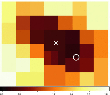
X-ray spectral index variation map of PWN 0540. The colour coding represents values of the spectral index αν, which varies from 0.65 to 1.8. North is up and east to the left. The white cross is the pulsar optical position, and the white circle is the optical aperture centred on the ‘blob’ position in 1999. Note that this region overlaps with the area which has the smallest spectral index, αν = 0.65 ± 0.03 (see Table 5), in X-rays. The distance between the pulsar and the blob is 1.4 arcsec.
As seen in Fig. 11, the blob demonstrates the hardest emission within the PWN. Its hardness even exceeds that of the pulsar, underlining the peculiarity of this structure. In general, the brighter the region, the harder its spectrum. This leads to the left–right asymmetry of the hardness of the PWN along the major axis clearly seen in Fig. 11, where the orientation of the north-east–south-west major axis slice is the same way as in Figs 7–9. The hardness profile along the minor PWN axis is, on the other hand, almost symmetrical, and demonstrates a gradual softening of the emission with distance from the pulsar, from α∼ 0.9 to ≳1.6. The hardness image (Fig. 10) does not reveal any hardening to extreme values for the assumed torus region, as seen in the Crab PWN (Weisskopf, Hester & Tennant 2000; Mori, Burrows & Hester 2004).
3.6 Multiwavelength spectrum of the ‘blob’ region
In Serafimovich et al. (2004) we studied the optical spectra for the 1999 HST/WFPC2 epoch of several positions in what we then defined the torus and jet of the PWN. One of these positions, called ‘Area 2’ in Serafimovich et al. (2004), turns out to partly overlap with the ‘blob’ discussed by De Luca et al. (2007). The results of Serafimovich et al. (2004) hint that the optical spectrum of their ‘Area 2’ in 1999 was different from other regions of the PWN since it could have had a somewhat steeper spectrum in the optical with αν = 1.58+0.33−0.30. In Table 4, the spectral slope of the ‘blob’ has αν = 1.35+0.27−0.22 for the same epoch. The overlap between ‘Area 2’ in Serafimovich et al. (2004) and the ‘blob’ in Table 4 is only ∼60 per cent. The results are, however, clearly compatible even within 1σ. How the optical emission of the ‘blob’ varies with time, if moving, as well as other regions how they vary with time, is discussed in Section 3.2, and listed in Table 4.
Perhaps of more general interest is to see how the optical emission connects to the emission at other wavelengths. In Serafimovich et al. (2004, their fig. 15), a comparison between the multiwavelength spectrum (radio to X-rays) from the entire PWNe of the Crab and 0540 was made. For both objects, an extension of the X-ray spectrum overshoots the optical spectrum in a log(ν) versus log(Fν) diagram. A further roll-off towards the radio is seen in both PWNe. A cubic spline fit for the entire logarithmic spectrum for the Crab PWN, overshoots both in the optical and radio for 0540, if fit to its X-ray part. We have done the same multiwavelength study here, but concentrating on the 0540 ‘blob’. The optical data are again from 1999, but for the X-ray data, we used our reductions of the 2006 Chandra data. These have better signal-to-noise ratio than earlier data. We could have chosen optical data closer in time to the 2006 Chandra data, but a look at Table 4 for all areas, except the ‘blob’, shows that the optical flux is stable between 1999 and 2007. For the ‘blob’ in Table 4 we applied 0.4 arcsec shift between 1999 and 2007, so the overlap between the 0.455 arcsec apertures for each epoch is fractional. Nevertheless, the flux in the red HST bands for the ‘blob’ in Table 4 is similar between 1999 and 2007 to within 5–10 per cent. We emphasize that the X-ray spectrum of the blob has been extracted from the same aperture position and extent as has been used for the 1999 optical flux measurements. For the absorbing gas column density NH we used the results of Section 3.5.
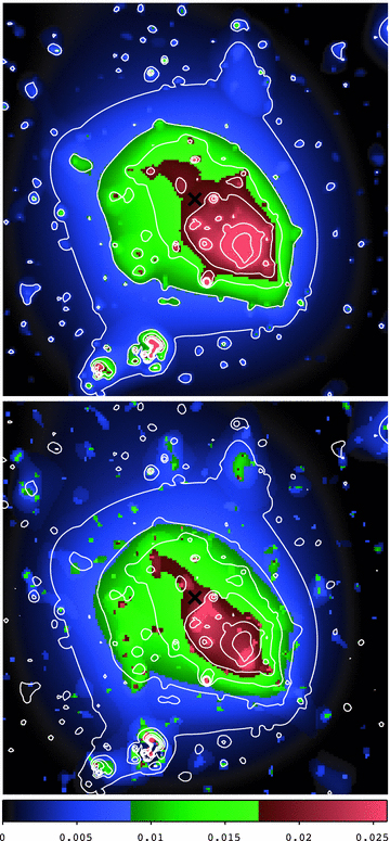
Upper: wavelet filtered continuum image of PWN 0540 obtained with HST/F547M in 1999 with overlaid contours. Lower: wavelet filtered continuum F547M in 2005 image with overlaid contours from the 1999 epoch. Note how the ‘blob’ structure and the structure just south-west of the pulsar change in morphology between these two epochs. For the structure close to the pulsar the strongest emission in the 2005 image is much wider than in the upper panel. The increased emission close to the pulsar could be new blob emerging.
The multiwavelength result is shown in Fig. 12. It is clear that an extension of the X-ray data, considering the rather well-determined X-ray slope, undershoots rather than overshoots the optical data. What stands out here, like in Serafimovich et al. (2004) for the whole PWN, is the intrinsically steep optical spectrum compared to the X-ray spectrum. We caution that the errors calculated, and shown in Fig. 12 for the optical data points, are the statistical errors only. If we would allow for a modest (12–15 per cent) systematic error of the F791W flux, one can connect all optical and X-ray data with a single power law to within 2σ. The slope of that power law would be αν = 0.74 ± 0.03, which is marginally different from the X-ray spectral slope with αν = 0.65 ± 0.03. As we noted above, at least part of the systematic error (5–10 per cent) may come from using the spatially slightly shifted 1999 optical data, rather than data closer to the epoch of the X-ray data, i.e. 2006.
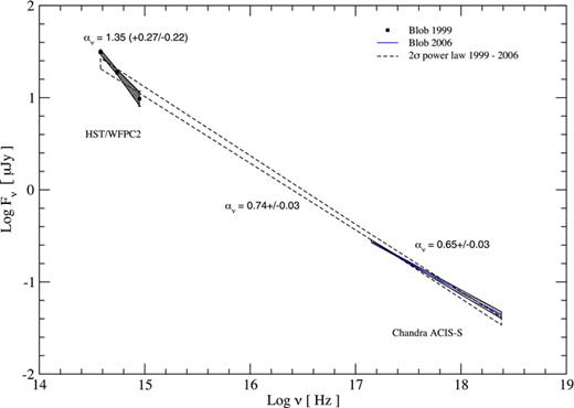
Multiwavelength spectrum for the ‘blob’ region. See text for details.
We emphasize that our finding that a single power law may fit the optical/X-ray part of the spectrum for 0540 was derived only for the ‘blob’, and therefore does not necessarily contradict our findings in Serafimovich et al. (2004) that spectral breaks are needed for the whole PWN. While we leave a discussion for the entire nebula for a future paper, we can make use of Figs 8–10 to check whether our reductions of Chandra data make a difference compared to the X-ray spectra used in Serafimovich et al. (2004). From Fig. 10 we note that the X-ray spectral index is in the range 1.4–1.8 in the north-west and south-east part of the PWN, and from Figs 8 and 9 that the optical and X-ray fluxes are ∼2 and ∼3–5 times weaker there, respectively, than at the ‘blob’ position. In Fig. 12 we show that a single power law with spectral index αν = 0.74 ± 0.03 could be enough for the ‘blob’. Using a difference of 3 dex between the optical and X-ray frequencies, an X-ray spectral index of αν = 1.6 would make an extension of the X-ray spectrum overshoot the optical by more than 2 dex in flux in the north-west or south-east parts of the PWN. A single power law for those regions is thus not possible, or actually in any part of the remnant where the X-ray spectral index is αν≳ 0.9. As αν≳ 0.9 is true for most of the PWN, a single power law for the whole PWN will not be possible, and our results will in this sense not contradict the findings of Serafimovich et al. (2004). From Fig. 10 we note that αν≲ 0.9 applies only along the major axis within ∼2 arcsec from the pulsar. The simplest explanation to this is that energy injections occur in this region, and that cooling of electrons takes place, thus steepening the X-ray spectrum, when electrons move away from this region.
4 DISCUSSION
4.1 Morphology of the PWN
The PWN of PSR B0540−69.3 and SNR 0540−69.3 have been imaged on several occasions. In Serafimovich et al. (2004) we concentrated on the continuum-emitting PWN, and images showing the line-emitting gas of the inner ∼4 arcsec of the SNR are nicely compiled in Morse et al. (2006). While there are some general features in common between continuum-emitting and line-emitting gas (like overall shape and concentration toward the south-west), there are also several important differences.
The line-emitting gas is concentrated to the south-west, but with distinctions between the spatial distribution of e.g. [O iii] and [S ii]. This can be seen in the wavelet filtered images from 1999 shown in Fig. 13. The [O iii] structure appears overall rounder in shape, whereas [S ii] is more focused to the south-western conglomerate, and shows only little emission to the north-east. A protrusion extending ∼2 arcsec outside the main body of the emission in the south-western direction is seen in both [O iii] and [S ii]. The structure of this is reminiscent of the Crab chimney. What is striking is that the protrusion connects to the area of strongest [S ii] emission in the remnant body, whereas the [O iii] emission in the remnant is in general weaker in the pulsar-protrusion direction, than in the areas east and west of it, i.e. the areas flanking the ‘blob’.
![Upper left: wavelet filtered [O iii] image of PWN 0540 obtained with HST/F502N in 1999 with overlaid contours from the continuum image in the upper right-hand panel. Upper right: wavelet filtered continuum image of PWN 0540 obtained with HST/F547M in 1999 with overlaid contours. The black cross shows the pulsar position. Lower left: wavelet filtered [S ii] image obtained with HST/F673N in 1999 with overlaid contours from the continuum image. Lower right: ratio map of [S ii]/[O iii], with [S ii] and [O iii] from the lower left- and upper left-hand panels, respectively. Overlaid contours are from the optical continuum in the upper right-hand panel. The scale at the bottom of the figure represents colour coding for that ratio image.](https://oup.silverchair-cdn.com/oup/backfile/Content_public/Journal/mnras/413/1/10.1111_j.1365-2966.2010.18159.x/1/m_mnras0413-0611-f13.jpeg?Expires=1749908616&Signature=dSrvbc09VwkfG8LTsU2LJ8WC~YTHqX2NSOfWlvXl1Sd4cQhwqIbfYitQfIDTzJmdZEkLPeKZ56huUKffWIB6lgaYQ2FvA5SFIEXIGsMGfjT5yYmBUnA46ChvXtCrA6G8SIn48P7TnWVD1YxrpNeNd23qGQWbkuFKmR3Ww4ghc3WyKGOOCR-4j28eJAfoBc32-aLlhRt9bMD-Lcpj0Ckhfn80Vta83iODbouuC5kPeHHTi2gq6Lj0KwT-p2fR8bC7AuSSM-zMWi25F-pc-J7hdlWK5~rF2h~xrCSfd6pJDtuiH~hQxzedP~Nn5f-B9~neWLE5WwibH2MtoBPU-u4ZmA__&Key-Pair-Id=APKAIE5G5CRDK6RD3PGA)
Upper left: wavelet filtered [O iii] image of PWN 0540 obtained with HST/F502N in 1999 with overlaid contours from the continuum image in the upper right-hand panel. Upper right: wavelet filtered continuum image of PWN 0540 obtained with HST/F547M in 1999 with overlaid contours. The black cross shows the pulsar position. Lower left: wavelet filtered [S ii] image obtained with HST/F673N in 1999 with overlaid contours from the continuum image. Lower right: ratio map of [S ii]/[O iii], with [S ii] and [O iii] from the lower left- and upper left-hand panels, respectively. Overlaid contours are from the optical continuum in the upper right-hand panel. The scale at the bottom of the figure represents colour coding for that ratio image.
The optical continuum emission from the same epoch, as exemplified by the uppermost right-hand panel in Fig. 13 and contours overlaid on the line-emission maps, is even more concentrated to the south-west than the [S ii] emission, but the overlap between [S ii] and the continuum is obvious. No clear indication of a protrusion is seen in the wavelet filtered continuum image, which could be due to lower signal-to-noise ratio. The overlap between optical continuum and regions of enhanced [S ii] emission is evidenced by the lower right-hand panel of Fig. 13, where we have made a ratio map of [S ii] and [O iii]. The highest optical continuum flux occurs in a conglomerate with a large [S ii]/[O iii] ratio. The correlation between optical continuum and the [S ii]/[O iii] ratio is indeed even more pronounced than with the [S ii] emission alone. This could either be a physical coincidence of continuum emission and regions of high sulphur abundance and/or lower state of ionization, or it could signal that shock excitation is more important in those regions compared to regions with smaller [S ii]/[O iii] ratios. Shocked gas generally emits more [S ii] than [O iii] compared to photoionized gas, and the temperature of the gas is higher (see Williams et al. 2008). A temperature higher than the equilibrium temperature in photoionization-dominated plasma can also be obtained in a time-dependent situation. An example is the flash photoionization of the inner ring around SN 1987A where the [O iii] temperature was ∼5 × 10⁴ K shortly after the outburst (see fig. 1 in Lundqvist & Fransson 1996). We explore this possibility further below.
The spatial distribution of the continuum emission in the PWN of 0540 shows high variability in the optical. This was noticed by De Luca et al. (2007), and they argued that the ‘blob’ shown in Fig. 14 had moved between 1999 and 2005. The change in the spatial distribution of the optical continuum is clearly seen in our wavelet filtered images in Fig. 15. Fig. 15 also shows how a new structure appears just south-west of the pulsar, as if a new ‘blob’ would be generated, whereas the overall structure does not differ between the two epochs. In addition, Fig. 15 shows how the structure extending from the pulsar (marked by a black cross) toward the ‘blob’ continues in the north-eastern direction, although with lower intensity and less extent.
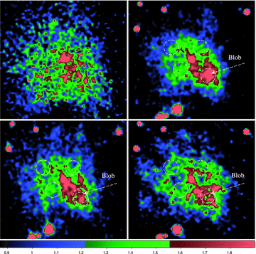
The PSR B0540−69.3 and its PWN obtained with HST/F547M in 1992 (upper left), in 1999 (upper right), in 2005 (lower left) and HST/F450W in 2007 (lower right). Note that the cut levels for the F540W image were compensated for the slope of the nebula’s spectral energy distribution (SED). The white circular apertures show the ‘blob’ position in 1999 and respective epoch, as well as three other areas selected for comparison. In the 2005 and 2007 images we have also made circular apertures for the 2005 position of the ‘blob’, and the expected 2007 position if the ‘blob’ displacement would be linear in time. Some stars projected on the PWN were subtracted off.
The soft X-ray emission has an even more remarkable concentration of emission to the ‘blob’ position than in the optical, with a soft X-ray flux as bright as ∼10 per cent of the pulsar emission. The X-ray position does not seem to vary appreciably with time between 2000 and 2006, and the X-ray spectrum is a power law which is hardest at the ‘blob’ position, and becomes increasingly softer away from it (see Fig. 10). In general, the spectrum is harder along the north-east–south-west direction than off this orientation. The optical continuum emission shares the general brightness distribution of the X-ray emission along the north-east–south-west direction, but it does also show strong variability of the spatial distribution. That we are able to see this in the optical, but not in X-rays, may be an effect of better spatial resolution.
4.2 Excitation of the line-emitting filaments close to the ‘blob’
The variability of the spatial distribution of the optical line emission is less known since observations through HST line filters have only been performed once, namely in 1999 (Morse et al. 2006). However, we also have some slit spectra taken in 1996, which partly sample the ‘blob’ region (Lundqvist et al., in preparation), and which do not indicate strong [S ii] emission at the position of the 1999 ‘blob’. This, together with the fact that the optical continuum emission does vary, suggests that the line emission may also vary with time.
The excitation of the line-emitting filaments is most naturally explained through shock activity (Williams et al. 2008), but in Section 4.1 we also highlighted the possibility of time-dependent photoionization. The idea is that the optical continuum activity could also indicate higher X-ray activity, and that the X-rays could photoionize unshocked filaments that are quasi-stationary. As we have seen, the X-ray emission from the ‘blob’ in 2006 is about a factor of 10 weaker than the emission from the pulsar, but we only wish to study the photoionization close to the ‘blob’ where X-rays from the ‘blob’ dominate, so to study whether time-dependent photoionization is important, we have ignored the pulsar X-rays.
To test the effect of time dependence we have made models where we have artificially switched on the X-ray emission from the ‘blob’ to study how it would photoionize nearby gas. The model is similar to that used in Lundqvist & Fransson (1996) for SN 1987A, but with several updates (see e.g. Mattila et al. 2010). We have assumed that the ‘blob’ is spherical with radius 0.2 arcsec, and that the gas being photoionized surrounds the ‘blob’ also in a spherical fashion. For the density of this gas we adopted the results of Serafimovich et al. (2005) who derived an electron density in the range 1–5 × 103 cm−3 from the [S ii]λλ6716, 6731 lines. For the abundances of the filaments we have assumed a composition with the relative abundances (by number) suggested by Williams et al. (2008), i.e. C:O:Ne:Mg:Si:S:Ar:Ca:Fe = 0.1:1:0.2:0.1:0.1:0.1:0.1:0.1:0.1. We have also blended in H and He at various amounts as Serafimovich et al. (2005, see also Morse et al. 2006) clearly revealed the presence of hydrogen. The ionizing luminosity from the ‘blob’, when switched on, is assumed to be 4.66 × 1031(E/1 keV)−0.65 erg s−1 eV−1. With H and He mixed in so that H:He:O = 1:1:1, and with a total density of atoms and ions nat = 1.5 × 103 cm−3, the ionization parameter (number density of ionizing photons divided by nat) is ∼10−3, i.e. only a thin rim of gas is photoionized around the ‘blob’. Steady state is reached in ∼10 yr, which is longer than the time-scale for changes in the ‘blob’ structure, justifying time dependence. Peak temperature of the ionized gas reaches ∼8.5 × 10³ K, and occurs already after 3 months. Maximum ionization occurs when steady state is being approached. Although sulphur is mainly in S ii, i.e. which we know from Fig. 13 is just what is observed in the ‘blob’ region, most of the oxygen is still in O i. This contrasts the observations of Kirshner et al. (1989) which show very weak [O i] emission. One must caution that the observations of Kirshner et al. were made more than one decade before the ‘blob’ in 1999, and that the slit of Kirshner et al. was not ideally placed to probe the ‘blob’ region. The very small ionization parameter and the low temperature of the ionized gas are, however, enough to make us rule out photoionization by X-rays from the ‘blob’ structure as a viable source for the excitation of the [S ii] emitting gas in the south-western part of the PWN. If we disregard the possibility that this region is truly more abundant in sulphur than other parts of the nebula, the remaining explanation is what is discussed by Williams et al. (2008), i.e. [S ii] being boosted by shock activity.
4.3 Is the ‘blob’ a moving entity?
In Fig. 14 we also include the epochs 1992 and 2007. The signal-to-noise ratio is too low in the 1992 data, which we have included for completeness, to draw any conclusions more than that the continuum emission is enhanced in the south-western direction. The 2007 image shows a much weaker ‘blob’, and it is in fact not obvious that the ‘blob’ structure is longer present in 2007. In general, the U-shaped structure in the 1999 image, with the pulsar at the upper left part of the U structure, and the ‘blob’ at the bottom, remains roughly intact between 1999 and 2005, but breaks up in 2007. A ‘blob’ structure so clearly seen in 2005 divides up into three fragments with the lower one roughly at the expected position of the ‘blob’, but with the strongest emission seen north-east of the 1999 ‘blob’ position. In 2005 that position is actually devoid of strong emission. One could imagine that this new structure in 2007 could signal propagation of the 2005 ‘blob’ just south-west of the pulsar, but we also note that the structure just north-east of the ‘blob’ in 2007 is clearly seen in 1999, but less brighter. A possibility is that the whole structure responsible for the continuum emission exists at all epochs, but that it contributes with different amounts at different epochs. With this interpretation, the northern part of the ‘blob’ is just an enhancement in emission in 1999, which then fades away, leaving only the southern part of the ‘blob’ seen in 2005, and even more so in 2007.
Our findings can therefore suggest that the ‘blob’ structure may not be a moving entity, but rather a part of the filamentary structure that was excited in 1999, and then fades in optical intensity. Particularly evident is how well the continuum emission traces the emission structure in [S ii] and how low the correlation is between continuum and [O iii] (see Section 4.1). The high [S ii]/[O iii] ratio suggests shocks (cf. Section 4.2), this possibility being strengthened by the fact that the ‘blob’ coincides with a position in the PWN where the polarization angle changes abruptly and where there is strong X-ray emission. A possibility is an outflow in the PWN from the pulsar which excites the filaments at the ‘blob’ position in a time-varying fashion. Another possibility is a local release of energy at the ‘blob’ position which then causes a point-like expansion of plasma. In both these cases there will be, after some delay, slow shocks transmitted into filaments embedded in the PWN in a way similar to the shocks transmitted into the blobs of the circumstellar ring around SN 1987A (e.g. Gröningsson et al. 2008).
As discussed in Section 3.3, there are several positions along the major symmetry axis (north-east–south-west) of the PWN where the polarized flux peaks other than at the ‘blob’ position, and where the polarization angle changes at these positions. This could be a sign of past, or weak present, shock activity. A possibility is that energy is released along this symmetry axis at different places at different epochs, which means that the ‘blob’ was just a recent such event. If the ‘blob’-like feature seen in 2005 just south-west of the pulsar is a new feature moving southward, the sporadic energy release scenario may prove wrong. If it breaks up, it could speak in favour of a sporadic energy release. Indeed, we note in 2007 a peak above 3σ at ∼0.6 arcsec in polarized flux, southward along the major symmetry axis (see Fig. 8), as well as a change in polarization angle. Looking at Fig. 14 from 2007, no obvious blob-like counterpart is seen at that position. This could hint that the 2005 ‘blob’-like feature broke up, leaving only an imprint on the polarization map.
We also note that the two strong peaks in polarized flux south-west of the pulsar occur in the protrusion-like feature most clearly seen in lower left-hand panel of Fig. 13 which shows wavelet-filtered [S ii] emission from 1999. The north-east–south-west slice in Fig. 8 catches the northern part of this protrusion. Further polarization studies would shed more light on this and other regions of the PWN. At the moment we only have good data from one epoch, namely the one from 2007 discussed here.
The strong spatial variation of the inferred X-ray power-law slope of the emitted radiation (cf. Fig. 10) shows that multiwavelength spectra should be studied over limited spatial extents. In Serafimovich et al. (2004) we invoked possible spectral breaks between the optical and X-rays when studying the multiwavelength spectrum of the full PWN. From Fig. 12 here, we argue that a single power law may be sufficient for the ‘blob’. A single power law could mean that the 1999 ‘blob’ position is a site of energy injection to relativistic electrons. Further multiwavelength, and preferably contemporaneous, studies at other positions, away from the ‘blob’, would reveal if a break in the power law appears, and if cooling of the electrons occurs. We leave this for a future study.
4.4 The supernova progenitor
The X-ray spectral analysis presented in Section 3.5 gave better results if we included ‘extra’ absorption from oxygen-rich gas in addition to the interstellar gas in the LMC and MW. The column density of extra oxygen we found to be needed was NSNRO≈ 3.1 × 1018 cm−2. Adopting SN 1987A, and particularly the model used in Blinnikov et al. (2000) and Serafimovich et al. (2004) as a model for 0540, NSNRO = 9.5 × 1017 cm−2 for an SN 1987A age of t = 800 yr, where the column density scales with age as t−2. It seems unlikely that 0540 is younger than 800 yr, so if NSNRO is indeed as high as suggested from our X-ray analysis, then more oxygen was produced in 0540 than in SN 1987A, and/or the oxygen-rich ejecta of 0540 expand more slowly or it could be differently mixed than in the model of Blinnikov et al. (2000). As we do not find any evidence for strong variation of the oxygen column density over the PWN, a higher than average column density along the line of sight to us is less likely.
It is interesting to note that the model used in Blinnikov et al. (2000) invokes ∼2 M⊙ of oxygen, whereas Williams (2010) in his PhD thesis argues for an upper limit of ∼3.5 M⊙ of oxygen. If the oxygen mass is this high in 0540, and the velocity structure of oxygen more ‘compact’ than in SN 1987A, NSNRO could be close to the value inferred from our X-ray extractions. A high oxygen mass would then favour a progenitor in the upper mass range for the ones discussed by Chevalier (2006), and we would end up with the same mass range of 20–25 M⊙ as favoured also by Williams (2010). We note that Park et al. (2009) did not need to include elevated levels of oxygen for the X-ray absorption, which does not contradict our indications. Their analysis was made for the outer parts of the SNR not covered by the oxygen-rich ejecta.
4.5 Future observations
To map out the 3D shock structure of the filaments, good resolution both in space and velocity is needed. Previous deep spectroscopic observations of 0540, partly used in Serafimovich et al. (2004, 2005) and discussed in a forthcoming paper (Lundqvist et al., in preparation, see also above), show no clear [S ii] activity close to the ‘blob’ position, but these observations were made prior to the knowledge about the ‘blob’, and the slits were not ideally placed to constrain the ‘blob’ activity. These observations were also carried out at seeing ≳1.1 arcsec. To map out the velocity structure of the ‘blob’ region in order to constrain the propagation of the shocks, observations with good spatial resolution and coverage are needed. Modern integral field units (IFUs) with a spectral resolution of (≲100 km s−1) are particularly useful, especially in good seeing and at low airmass. The good velocity resolution is useful to separate out slow (tens of km s−1) shocks driven into the filaments from the faster (∼250 km s−1) shocks driven into more hydrogen-rich gas (cf. Williams et al. 2008). Observations in the optical should also be sensitive enough to catch weaker lines like [O iii]λ4363 for temperature estimates.
The ‘blob’ in the south-west part of the PWN, first seen in 1999, was truly an extraordinary event. As we have argued for above, similar events may, however, have occurred also in the past. Continuous imaging monitoring of 0540 is therefore important, both in the continuum and in lines like [S ii] and [O iii], to see if new blobs emerge. HST can continue to play an important role here, especially with the upgrade to WFC3 which has no CTE effects. To see how polarization evolves would be particularly useful for a global picture of the PWN. Further down the line, both JWST and ALMA with their good sensitivity and spatial resolution will provide very important links between optical and radio studies of the PWN of 0540. Such studies at good angular resolution will also make it easier to compare 0540 to its much closer twin, the Crab.
Multimission Archive at STScI, http://archive.stsci.edu
Hubble Space Telescope Archive at Canadian Astronomy Data Center, http://www.4.cadc-ccda.hia-iha.nrc-cnrc.gc.ca/hst
Space Telescope European Coordinating Facility, http://archive.eso.org/cms/hubble-space-telescope-data
Space Telescope Science Data Analysis System, http://www.stsci.edu/hst/wfpc2/documents/dither_handbook.html
The frame time of the 1/4 mode is ≲1.1 s, for details see http://asc.harvard.edu/proposer/POG/html/chap6.html
USNO-B1 is currently incorporated into the Naval Observatory Merged Astrometric Data Set (NOMAD) which combines astrometric and photometric information from Hipparcos, Tycho-2, UCAC, Yellow-Blue6, USNO-B and the 2MASS, http://www.nofs.navy.mil/data/fchpix
We would like to thank the referee for important remarks that helped to clarify the text. We also thank Jennifer Mack Research and Instrument Scientist in the ACS/WFPC2 team at the Space Telescope Science Institute for the assistance with calibration of the HST/WFPC2 data, and Jean-Luc Starck for discussions. PL and C-IB acknowledge support from the Swedish Research Council, and GO support from Swedish National Space Board. YAS and DAZ were partly supported by RFBR (grants 08 02 00837 and 09 02 12080) and by the State Programme ‘Leading Scientific Schools of RF’ (grant NSh 3769 2010.2). DAZ was also supported by a St. Petersburg Government grant for young scientists.
REFERENCES
