The kinematic component of the cosmological redshift Free

Abstract

1 INTRODUCTION

A standard interpretation of the cosmological redshift in the framework of the Friedman–Lemaître–Robertson–Walker (FLRW) models is that it is an effect of the expansion of the Universe. This interpretation is obviously correct since 1 +z=a(t_o)/a(t_e), where z is the value of the redshift, a(t) is the scalefactor of the Universe and t_e and t_o are respectively the times of emission and observation of a sent photon. In semipopular literature (e.g. Kaufmann & Freedman 1999; Fraknoi, Morrison & Wolff 2004; Seeds 2007), but also in scientific literature (e.g. Harrison 2000; Abramowicz et al. 2007), one can often find statements that distant galaxies are ‘really’ at rest and the observed redshift is caused by the ‘expansion of space’. According to other authors (e.g. Peacock 1999; Whiting 2004; Chodorowski 2007a,b; Bunn & Hogg 2009, hereafter BH9), such statements are misleading and cause misunderstandings about the cosmological expansion. A presentation of the debate going on in the literature on this issue is beyond the scope of the present work; a (possibly non-exhaustive) list of papers in this debate includes Davis & Lineweaver (2001, 2004), Barnes et al. (2006), Francis et al. (2007), Lewis et al. (2007, 2008), Grøn & Elgarøy (2007), Peacock (2008), Abramowicz et al. (2009), Chodorowski (2008) and Cook & Burns (2009).

On the other hand, there is broad agreement that the cosmological redshift is not a pure Doppler shift; the gravitational field must also generate a gravitational shift. Gravity can be neglected only locally, in the local inertial frame (LIF) of an observer. It turns out that for small redshifts, the cosmological redshift can be decomposed into a Doppler shift and a Newtonian gravitational one (Bondi 1947). The latter is a shift induced by the Newtonian gravitational potential. Can the cosmological redshift be decomposed into a Doppler shift and a gravitational shift (not necessarily Newtonian) for an arbitrary value of the redshift? This is the question which we want to deal with in this paper. Formally, the answer is no. There is no invariant definition of the recession velocity of a distant galaxy in general relativity (GR). This velocity is a relative velocity of the galaxy and the observer, and in curved space–time there is no unique way to compare vectors at widely separated points. A natural way to define the recession velocity is to transport parallelly the velocity four-vector of the distant galaxy to the observer, but the result will depend on the chosen path. (This is just the definition of curvature.) In practice, however, as a ‘preferred’ path one can choose a geodesic connecting the galaxy and the observer. Moreover, in FLRW models there is a natural foliation of space–time, into space-like hypersurfaces of constant cosmic time. For the geodesic in our paper, we will adopt the geodesic lying on such a hypersurface, i.e. connecting the points of intersection of the world-lines of the galaxy and the observer with the hypersurface of constant cosmic time.

In a seminal study of the cosmological redshift, BH9, following Synge (1960) and Narlikar (1994), another geodesic was adopted for the parallel transport: the null geodesic, along which the photon is travelling from the source to the observer. This approach results in one ‘effective’ velocity, while we think it is important to make a distinction between the velocity at the time of emission and the velocity at the time of observation. These two velocities are obtained by transporting parallelly the velocity four-vector of the source respectively on the hypersurface of constants t_e and t_o. Not surprisingly, our results differ from those obtained by BH9. However, unlike theirs, ours correctly reproduces the small-redshift decomposition of the cosmological redshift into a Doppler component and a gravitational component, mentioned above. Specifically, our decomposition coincides with that of Bondi (1947) for isotropic and homogeneous matter distribution.

This paper is organized as follows. In Section 2 we transport parallelly the velocity four-vector of a distant galaxy to the observer. From the transported vector we calculate the recession velocity of the galaxy, which turns out to be dependent on the galaxy’s comoving distance and the assumed background cosmological model. In Section 3 we find specific relations between the cosmological redshift and its Dopplerian component for two particularly simple cosmological models: the empty model and the Einstein–de Sitter model. In Section 4, using only the Principle of Equivalence, we derive the small-redshift decomposition of the cosmological redshift and find it to be identical with that obtained in Section 3 using generally relativistic approach. In Section 5 we calculate the recession velocities in the two models mentioned above, as well as for the currently favoured, flat non-zero Λ model with Ω_m = 0.24. We also find that the velocities are subluminal in all FLRW cosmological models and for all values of the redshift. A comparison of the results obtained in this work with results obtained in some earlier works on the subject is given in Section 6. Summary is presented in Section 7.

2 PARALLEL TRANSPORT

The equation for parallel transport of a vector U along a curve with a parameter λ and a tangent vector U={dx^μ/dλ} is

1

Here, Γ^α_μβ are the Christoffel symbols, related to the underlying metric by the equation

2

The metric considered here is the FLRW metric. In the Robertson–Walker (RW) coordinates, it is

3

Here,

4

and k R⁻²₀ is the present curvature of the universe. For a closed, flat and open universe, respectively, k=+1, 0, −1, and the function S(x) equals sin (x), x, and sinh (x). Time t is the cosmic time, that is the proper time of all fundamental observers partaking in the homogeneous and isotropic expansion of the cosmic substratum (fluid). The scalefactor a(t) relates fixed, or comoving, coordinates, x, to physical, or proper, coordinates, r: r=ax. The RW coordinates are {x^μ}={ct, x, θ, ϕ}.

The curve considered here is a radial geodesic on the hypersurface of constant cosmic time, hence dx^μ=δ^μ₁dx, where δ^μ_ν is the Kronecker delta. This gives

5

The vector U is here the four-velocity of a distant galaxy, parallelly transported to the central observer (i.e. to the origin of the coordinate system). By definition, U^α = dx^α/ds, where x^α(t) denotes the galaxy world-line as a function of the cosmic time. In the RW (comoving) coordinates every galaxy has fixed θ, ϕ and x, so ds=c dt and U^α = dx^α/d(ct). For these reasons, the initial value for U^α is δ^α₀. Specifically, the initial conditions for equation (5) are

6

where x_* is the comoving radial coordinate of the emitting galaxy.

We calculate Γ^α_1β using equations (2) and (3) and obtain the following set of two linear equations for U⁰ and U¹:

7

8

We remind that since t is fixed, so are a and H. The corresponding equations for U² and U³ are simple to solve; with conditions (6), the result is U²(x) =U³(x) = 0. Differentiating equation (7) with respect to r and using (8) to eliminate dU¹/dx yields

9

The solution is

10

where C₁ and C₂ are the integration constants. Imposing initial conditions and noticing that we obtain

11

12

hence

13

14

We see that (g_αβU^αU^β)|_{x = 0} = 1, as it should.

In order to identify the transported velocity four-vector of the distant galaxy with its recession velocity, we now have to transform the vector from the RW coordinates to the coordinates of the local inertial frame (LIF) of the central observer. A general coordinate transformation transforms the (unprimed) components of the metric, g_αβ, to

15

The following transformation of the RW coordinates: t′=t, x′=a(t)x, θ′=θ, ϕ′=ϕ, yields which in the limit x′→ 0 tends to ⁠, i.e. to the Minkowski metric.1 Thus, the primed coordinates are indeed the coordinates of the observer’s LIF. A transformation of vector components, ⁠, yields here and ⁠, hence

16

17

Again, the components are properly normalized: ⁠.

In the LIF of the observer, the radial component of the parallelly transported four-velocity of the distant galaxy is non-zero. We interpret this effect as a non-zero recession velocity of the galaxy, v. Quantitatively, and ⁠, where β≡v/c and γ≡ (1 −β²)^−1/2. This yields immediately

18

19

hence2

20

Finally, since sinh y+ cosh y = exp y, we obtain

21

where z_D is the Dopplerian component of the (total) cosmological redshift of the galaxy, z. In Section 3 we will explain how to use this equation to relate the cosmological redshift of a distant galaxy to its Dopplerian component. Equation (21) is the central formula of the present paper.

3 REDSHIFTS FOR SPECIFIC MODELS

Let us remind that in equation (21), x_* stands for the comoving radial RW coordinate of a galaxy. For simplicity, from now on we will denote this coordinate by x. In fact, x is not only a coordinate but also the comoving radial proper distance to the galaxy and can be expressed in terms of the redshift of the galaxy. For a given cosmological model, the relation between x and z is determined by the Friedman–Lemaître (FL) equations. Using this relation and equation (21) enables one to deduce the relation between z and z_D in this model. In the following, we will find the relation between z and z_D for two specific, particularly simple cosmological models.

Formula (21) is valid for any (fixed) value of cosmic time. Two instants of time are of interest: the time of observation, or ‘today’, t_o, and the time of emission, t_e. The corresponding values of the recession velocity are respectively v_o=v(t_o) and v_e=v(t_e).

3.1 Time of observation

At the time of observation (we use the normalization a_o = 1, so that the comoving radial distance equals the proper distance as it is today), hence

22

Here, z_D is a Doppler shift due to the present value of the recession velocity, v_o.

3.1.1 Empty universe

In the empty model (Ω_m=Ω_Λ = 0), the comoving radial distance is x(z) =c H⁻¹₀ ln(1 +z), hence e^{ln (1 +z)} = 1 +z_D, or

23

In an empty universe the origin of the cosmological redshift is thus entirely Dopplerian. This result is expected, since space–time of an empty universe is the Minkowski space–time, where redshift is simply a Doppler shift.

Some cosmologists still believe that the cosmological redshift is not a Doppler shift even in the case of an empty universe. The origin of this erroneous belief is a wrong interpretation of the FLRW metric for an empty universe in the RW coordinates. In these coordinates, space (3-D hypersurface of constant cosmic time) does have a non-zero curvature, but what matters here is the full 4D curvature, which is zero. Indeed, a simple coordinate transformation transforms the metric to the standard Minkowskian form. What else could space–time of an empty universe be? There is no matter, so there is no gravity, and a complete relativistic description is provided by special relativity. Indeed, Chodorowski (2007a) proved that in an empty universe z=z_D, using only specially relativistic concepts. More specifically, he showed that 1 +z_D=a(t_o)/a(t_e), where a(t) =t/t_o is the scalefactor of the empty model. Another derivation of the redshift in the empty model will be presented in Section 4.

There is some remaining subtlety here that deserves further explanation. In the specially relativistic formula for a Doppler shift, ⁠, the recession velocity v is an inertial velocity of a distant galaxy, which we call v_distant. The velocity that appears in equation (21) and the resulting (23) is a ‘local’ velocity, v_local, transported parallelly from the galaxy to the central observer using the RW coordinates. Are these two velocities equal? Redshift is an observable, so the answer is ‘they must be’, but let us understand, why.

In Minkowski, i.e. flat, space–time, components of a transported four-vector in inertial coordinates are constant (see equation 1), so (i.e. transported) is equal to ⁠. Here, double primes denote the global inertial coordinates of the central observer, in which v_distant is measured. This equality is no longer true for non-inertial coordinates (like RW), but parallel transport does not depend on the coordinate system used, so the transported vector is the same. We have transformed the RW components of the transported four-velocity, U^α_local, to the components in the coordinates of the LIF of the observer, ⁠, and obtained v_local. Since the global inertial frame of the central observer is an extension of its LIF (possible only in an empty universe), and are the components of the same vector in the same coordinate frame, so they must be equal. We thus have ⁠, hence v_distant=v_local.

Summing up, our definition of the recession velocity of a distant cosmological object correctly implies that in the case of an empty universe the origin of the cosmological redshift is purely Dopplerian.

3.1.2 Einstein–de Sitter universe

In the Einstein–de Sitter (EdS) model (Ω_m = 1 and Ω_Λ = 0), the comoving radial distance is x(z) = 2 c H⁻¹₀ [1 − (1 +z)^−1/2], hence

24

The particle horizon for the EdS model is x(z=∞) = 2 c H⁻¹₀. We see that the Dopplerian component of the infinite cosmological redshift of a source located at the horizon sphere is z_D = e² − 1. This finite value corresponds to the recession velocity of the source not at the time of emission of photons (i.e. t_e = 0), but today. In Section 3.2.2 we will see that at t_e = 0, this velocity was c. The difference between the two velocities is due to deceleration of the EdS model.

3.1.3 Small redshifts

A second-order expansion in redshift of the radial distance valid for any cosmology (under the assumption that dark energy is in the form of the cosmological constant) is x(z) ≃c H⁻¹₀ [z− (1 +q₀)z²/2], where q₀≡Ω_m/2 −Ω_Λ. (It is easy to check that second-order expansions of the exact formulae for the empty and EdS models are consistent with this general expansion.) From equation (21), after expansion we obtain z_D≃z−q₀z²/2, or

25

In Section 4 we will see that the above result is identical to that obtained using the Principle of Equivalence (PoE).

3.2 Time of emission

At the time of emission, ⁠, where H_e is the Hubble constant at the time of emission. Using this equality in formula (21) we obtain

26

Writing the above we have used the fact that there is a unique correspondence between t_e and z, so H_e can be expressed in terms of the latter. A general formula for the Hubble constant as a function of redshift is

27

Here, Ω=Ω_m+Ω_Λ. In equation (26), z_D is a Doppler shift due to the recession velocity at the time of emission, v_e.

3.2.1 Empty universe

From equation (27) we obtain H(z) =H₀(1 +z), hence H(z)x(z)/[c(1 +z)] = ln(1 +z). This yields again

28

Equations (28) and (23) involve two different Doppler shifts: respectively at the time of emission, z_{D, e}, and at the time of observation, z_{D, o}. These equations are consistent because in the empty model the expansion of the universe is kinematic and recession velocities are constant in time. This is not true of any other cosmological model.

3.2.2 Einstein–de Sitter universe

In the EdS model H(z) =H₀(1 +z)^3/2, hence

29

The infinite value of z corresponds to the infinite value of z_D, so at the time of the big bang (corresponding to z=∞), the horizon was receding from the observer with the velocity of light. Let us decompose the cosmological redshift into a Doppler shift and the ‘rest’, z=z_D+‘rest’. From equation (29) we see that for high redshifts, the Dopplerian component of the cosmological redshift is (much) bigger than the total value of the latter. Therefore, in the EdS model the ‘rest’ must in fact be negative, i.e. it is a blueshift. We will show later that for small redshifts, the ‘rest’ can be identified with a gravitational shift. It will be demonstrated that a gravitational shift is indeed a blueshift for all matter-only models. A homogeneous and isotropic distribution of ordinary matter creates a gravitational potential well with the observer at the centre and the work performed by photons climbing down this well is negative.

3.2.3 Small redshifts

From equation (27) we have ⁠, hence H(z) x(z)/[c(1 +z)]≃z+ (q₀− 1)z²/2. Inserted in equation (26), this yields

30

Again, in Section 4 we will see that the above result is identical to that obtained using the PoE.

4 PRINCIPLE OF EQUIVALENCE

In Section 3 we studied the cosmological redshift using generally relativistic concepts. In this section we will restrict our analysis to small values of the cosmological redshift; this will allow us to use the PoE. It is well known that the PoE enables one to study local effects of light propagation in a weak gravitational field. Specifically, one can replace a static reference frame in this field by a freely falling frame in empty space. From the PoE it follows that the latter is locally inertial, with the laws of light propagation being given by special relativity. The classical examples of phenomena studied in this way are the gravitational redshift and the bending of light rays. In some instances it is possible to calculate correctly non-local effects by summing up infinitesimal contributions from adjacent local inertial frames, freely falling along the light ray trajectory. For example, the (small) gravitational redshift of a photon sent from the surface of a non-relativistic star (like, e.g. the Sun) to infinity can be calculated in this way. In some other instances it is not possible; a classical example is the bending of light rays. The calculation based on the PoE gives only half of the value of bending predicted by GR in the weak-field approximation [but see Will (2006) and references therein].

It is well known that the cosmological redshift can be interpreted as ‘an accumulation of the infinitesimal Doppler shifts caused by photons passing between fundamental observers separated by a small distance’ (Peacock 1999; see also Padmanabhan 1993; Peebles 1993). The derivation is very simple but let us recall it here. Consider two neighbouring comoving observers, located on the trajectory of a light ray, separated by an infinitesimal proper distance δl=a(t)δx, where a(t) is the scalefactor and δx is their comoving separation. The velocity of the second observer relative to the first is ⁠. The equation for the radial light propagation in the RW metric is c δt=aδx, where δt is the light traveltime between the two observers, so δv=c δa/a. This small recession velocity of the second observer causes a non-relativistic Doppler shift of the passing ray, δλ/λ=δv/c=δa/a. [Reference frames of the fundamental observers (FOs) are locally inertial.] Integrating the relation between λ and a we obtain 1 +z≡λ_o/λ_e=a_o/a_e.

The above derivation resembles a derivation using the PoE, which will be presented below. There is, however, an important difference. In the above we have applied the generally relativistic RW metric and the law of light propagation in it. The RW coordinates are local inertial coordinates of (freely falling) FOs and the cosmic time t is their local proper time. This has enabled us to integrate the effect (along the ray’s trajectory) trivially and exactly. Not surprisingly, then, the result is correct for an arbitrary value of the redshift. In an application of the PoE, the gravitational field of the system under consideration is described in terms of non-relativistic Newtonian dynamics, so the field must be weak. In the FLRW cosmological models the gravitational field is weak only at small distances from an observer, more specifically much smaller than the Hubble radius. Therefore, the PoE can give correct predictions only for small values of the cosmological redshift. Still, we think that calculations using the PoE are worth performing. The reasons are as follows.

First, the aim of our paper is to decompose the cosmological redshift into a global Doppler shift (i.e. due to the relative velocity of the emitter and the observer) and the ‘rest’. In the above calculation of the redshift we summed up contributions from infinitesimal relative velocities of neighbouring FOs, but this did not help us to express the answer in terms of the relative velocity of the emitter and the observer. As has already been stated many times, for large cosmological distances the recession velocity a priori is not well defined. In this paper we propose its generally relativistic definition. This definition is, however, quite formal, while for small redshifts, velocity is a well-defined pre-relativistic concept. Therefore, the identification of a global Doppler component of the small cosmological redshift will be simple and unambiguous. Second, in previous sections, using GR, we have shown that the cosmological redshift, of any value, can indeed be decomposed into a Doppler shift and the ‘rest’. In this section, using the PoE, we will similarly decompose the redshift into a global Doppler shift and the rest and will show that the ‘rest’ is the gravitational redshift in the Newtonian sense. In other words, we will prove that for small redshifts the rest is a classical Newtonian gravitational shift.

Among all the FLRW models there is a toy model which can be described using special relativity only. This is the empty, or Milne model (Milne 1993). At first sight, the relation of this model to the PoE is problematic, since in an empty universe there is no gravity. However, the relevance of the model will be seen later. Space–time of an empty universe is the Minkowski space–time. Let us denote the global inertial coordinates of an observer by T, X, Y and Z. In the standard spherical coordinates, R, Θ, Φ, the metric is

31

Like above, we will calculate the cosmological redshift summing up the infinitesimal Doppler shifts caused by photons passing between neighbouring FOs, located along the photons’ path. We have seen that such a summation can easily be done in the RW coordinates, for any FLRW model. However, it turns out that in the empty model, it is possible to perform this summation also using the Minkowskian coordinates T and R.

In the Milne model the recession velocities of FOs are constant; for example, in the rest-frame O of the central observer v(T, R) =R/T=H(T)R = const. Let us consider an FO located at a distance R from the central observer at time T. In his rest-frame O′, he observes a small Doppler shift of a photon sent (in fact, transmitted) by a nearby observer located at R+δR. Due to the Hubble expansion, the latter observer has a small recession velocity δv′=δR′/T′=H(T′)δR′ relative to the former. Like in the RW coordinates (locally coinciding with the coordinates T′ and R′), the relative wavelength shift is δλ/λ=δv′/c. However, in the empty model we can use the special-relativistic law of composition of velocities to relate the velocity δv′ to the velocity δv, measured in the observer’s frame O. This law can be applied, because the relative velocity of the frames O and O′, v(T, R), is constant. We have

32

hence we obtain

33

Let us denote the distance of the source at the time of emission by D_e. Our present task is to integrate this equation along the photon’s trajectory, c(T−T_e) =D_e−R. (The photon travels towards the central observer.) However, it can easily be checked that since the velocity of any FO is constant, δv(T, R) =H(T)δR equals to δv_e=H(T_e)δR_e. Therefore, the integration simplifies to an integration over R_e at fixed T=T_e,

34

(The minus sign accounts for the fact that for a photon travelling from the source to the observer R decreases, so δR is negative.) Defining β≡H_eR_e/c and β_e≡H_eD_e/c, we obtain

35

The left-hand-side integral is equal to ln(1 +z). The integration of the right-hand side (RHS) is elementary and yields ln[(1 +β_e)/(1 −β_e)]/2. Hence

36

In sum, we have accumulated infinitesimal Doppler shifts using the inertial coordinates of the central observer and expressed the total redshift in terms of the recession velocity of the source. The relation between the cosmological redshift and the recession velocity turned out to be given by the relativistic Doppler formula, in agreement with generally relativistic equation (28). Thus, as already stated earlier, in an empty universe the cosmological redshift is entirely a global Doppler shift. A similar derivation of the redshift in the empty model using Minkowskian coordinates with an explicit integration along the photon’s trajectory was presented in appendix A and section 2 of Chodorowski (2007a).

Now we proceed to derive, using the PoE, the relation between the recession velocity of a nearby source and its redshift, for non-empty universes. Why was the exercise with the Milne model useful for this purpose? High redshifts correspond to relativistic velocities and in the empty model their effects manifest as the 1 −β² factor in the integrand on the RHS of equation (35). Expansion of this integrand for small velocities and subsequent integration yields ⁠. Therefore, in our non-relativistic calculations we will be allowed to retain terms up to second order in β_e. (We will see later that the leading-order contribution to the velocity–redshift relation coming from Newtonian gravity is already of the second order in β_e.) Like previously, we denote Newtonian coordinates of the central observer by T and R. They are now inertial only locally, because there is a gravitational field. We ‘transform this field away’ using local inertial frames of FOs. Contrary to the empty model, FOs do not move now with constant speeds. According to the Newtonian interpretation of the FL equations (Milne & McCrea 1934), the change of speed of any FO located on a sphere centred on another observer is induced by the gravitational force exerted on the FO by the mass encompassed within this sphere. (This is Newton’s theorem for an isotropic and homogeneous universe. The speed of the FO is, of course, measured relative to the central observer). The effects of the cosmological constant Λ can be incorporated easily because Λ results in a force proportional to distance, similarly to the classical gravitational force for a homogeneous mass distribution. The FO located at time T at a distance R from the central observer has velocity related to his velocity at the time of emission of a photon, v_e, in the following way:

37

Here, T_e is the time of emission, R_e=R(T_e), ΔT=T−T_e and g(T_e, R_e) is the initial gravitational acceleration of the FO. Writing the above formula, we have approximated the changing acceleration of the FO by its initial value. [The result of this approximation for v(T, R) is already of second order in ΔT.] It is straightforward to calculate g(T, R) from Newton’s theorem and to express it in terms of the cosmological parameters. However, there is a faster way of doing this: by differentiating the Hubble law in Newtonian coordinates, v=H(T)R, with respect to time. The result is

38

where q is the deceleration parameter.

From equation (38), g(T_e, R_e) =−q_eH²_eR_e≃−q₀H²_eR_e. Inserting these expressions for v_e and g in equation (37), up to terms linear in ΔT we obtain:

39

(R≃R_e+H_eR_eΔT). The velocity of an FO is described here in terms of T and his initial position, R_e. A small relative velocity of two neighbouring FOs at time T, δv_|T, can be expressed as (∂v/∂R_e)_|TδR_e=H_e(1 −q₀H_eΔT)δR_e. This relative velocity causes a non-relativistic Doppler shift of the frequency of a passing photon. To obtain the total redshift we need to integrate these infinitesimal Doppler shifts along the photon’s path (i.e. null geodesic). Unlike in the empty model, here T and R are only locally inertial coordinates. However, their extent is quite limited, D_e≪c H⁻¹_e, so H_eΔT equals H_e(D_e−R)/c≃H_e(D_e−R_e)/c plus terms already of higher order in (D_e−R_e)/c. Therefore, equals

40

where, as before, β_e=H_eD_e/c. Hence we obtain finally

41

Expansion of the Doppler formula (36) to second order in β_e gives z_D=β_e+β²_e/2. Therefore, the first two terms on the RHS of equation (41) can be identified with a (global) Doppler shift due to the recession velocity of the source at the time of emission. Since the third term is of second order in β_e, we can write ⁠. In such a way we find out that equation (41) is identical to equation (30), the latter derived using a generally relativistic approach. In equation (25), the kinematic component of the redshift is related by the Doppler formula to the recession velocity of the source at the time of observation. We recover this equation by noting (with some small labour) that equation (39) yields β_e=β_o+q₀β²_o, and using this equality in equation (41).

The term −q₀β²_e/2 is a gravitational shift: the work, per unit-mass rest energy, performed by a photon travelling from the source to the observer. From equation (38) we have g≃−q₀H²_eR, so the gravitational potential Ψ(R) ≃q₀H²_eR²/2 + const. We thus indeed obtain (Ψ_o−Ψ_e)/c²=−q₀β²_e/2. Whether the observer is located at the centre of a potential well or on the top of a potential hill depends on the value of q₀. For all matter-only cosmological models q₀ is positive, so the observer is at the centre of a potential well. Then a gravitational shift is negative, so it is in fact a blueshift. This reflects the fact that the photon climbs down a potential well so the performed work is negative. For an accelerating universe (like, as we currently believe, ours) q₀ < 0 and a gravitational shift is a redshift.

Peacock (1999) derived equation (41) in a much simpler way. He stressed that in the definition of the redshift, the wavelength at the time of emission is the wavelength measured in the source’s rest-frame O′, λ_e′. In the observer’s rest-frame O this wavelength is Doppler-shifted, λ_e/λ_e′ = 1 +z_D. Next, on the path to the observer the photon undergoes a gravitational shift, λ_o/λ_e = 1 +z_G. Hence, 1 +z≡λ_o/λ_e′ = (1 +z_D)(1 +z_G). This equality gives formula (41) because, as we have verified above, z_G=−q₀β²_e/2, and because z_Dz_G is already of third order in β_e. However, freely falling observers employed in his calculation of z were not, strictly speaking, the freely falling observers of the studied problem. In the RW models freely falling observers are (by definition) FOs, partaking in the Hubble expansion. Peacock employed the standard ‘Einstein-lift’ observers, starting to fall only when the photon passes the top of their cabin. Accounting for non-zero initial velocities of freely falling observers complicated our calculations, but enabled us to apply the PoE ‘from first principles’. We performed our calculations consistently in the same way as we did using global inertial coordinates in the empty model, and the RW coordinates in all FLRW models.

Peacock’s aim was to derive a formula for the angular diameter distance up to the terms quadratic in redshift. In order to obtain the correct result, he had to expand the relativistic Doppler formula up to the term quadratic in β_e. Strictly speaking, this term is a relativistic correction and in principle one is not allowed to account for it in the calculations using the PoE, where velocities are assumed to be non-relativistic. However, the justification for including this term can be found analysing our calculations in the Milne model. We obtained ⁠, or ⁠, where was the lowest-order relativistic correction. Therefore, solving for z_D we were allowed to expand the exponential function up to a term quadratic in β_e, still remaining in the non-relativistic regime. Since the exponential function has the same second-order expansion as the Doppler formula, we correctly obtained the second-order Doppler relation, also in our non-relativistic calculations for non-empty models (see equation 41).

We stress that we did not assume that z=z_D+z_G. In our calculations both terms appeared naturally as a result of an application of the PoE. The first person to note that the cosmological redshift, if small, can be decomposed into a Doppler shift and a gravitational shift was Bondi (1947). He performed such a decomposition in a spherically symmetric generalization of the RW models, the Lemaître–Tolman–Bondi model. Our formula (41) is a special case of his formula (52), in a sense that z_G=−q₀β²_e/2 only for a homogeneous distribution of cosmic matter and small distances.

In the approach presented in this section, the cosmological redshift of any value is generated by relative motions of FOs. For small values of the redshift the application of the PoE allowed us to decompose the redshift into a Doppler component and a gravitational component.3 We have found that a Doppler component of the redshift is obviously generated by a kinematic component of the motions, while a gravitational component of the redshift is generated by their varying-in-time component. Of course, this interpretation of a gravitational component is fully consistent with the standard interpretation of a gravitational shift, because this is a gravitational field that causes FOs to accelerate.

5 RECESSION VELOCITIES

Calculations in Section 2, based on our definition of recession velocity, led us to equation (20). This equation is a general formula for the recession speed of a galaxy, valid for an arbitrary comoving position of the galaxy and an arbitrary instant of time. The hyperbolic tangent on the RHS of this equation ensures that the recession velocity of a source with an arbitrarily high redshift is subluminal (v < c). However, it is widely believed that recession velocities of sufficiently distant galaxies can be, and indeed are, superluminal (e.g. Davis & Lineweaver 2001, 2004; Grøn & Elgarøy 2007; Lewis et al. 2007). In Section 5.1 we will find a relation between our recession velocity and a commonly used estimator of the velocity: the proper recession velocity. Basing this relation we will show that the conception of the superluminal expansion of the Universe is wrong. In Section 5.2 we will intercompare our recession velocities of galaxies for some specific cosmological models.

5.1 No superluminal velocities

Let us remind that in the comoving coordinates {x^μ}={ct, x, θ, ϕ}, the FLRW metric takes on the form given by equation (3). For a particle (or a galaxy) participating in the homogeneous and isotropic expansion of the cosmic fluid, θ = const, ϕ = const and x = const. Hence, ds=cdt and

42

Let us change coordinates to ⁠, where r=a(t)x. Space–time interval ds is an invariant, so also in the primed coordinates ds=c dt. The four-velocity of the galaxy in these coordinates is

43

where is the Hubble constant.

It is a standard practice in the literature to use as an estimator of the recession velocity of a galaxy its so-called proper recession velocity,

44

that is the derivative of the proper distance between the galaxy and the observer with respect to the proper cosmic time. Comparing equation (43) with (44) we see that

45

or that v_prop/c is nothing more than the radial component of the galaxy’s four-velocity in the proper coordinates {ct, r, θ, ϕ}. Therefore, the proper velocity can indeed attain superluminal values,4 but should not be regarded as a recession velocity. As described earlier, to calculate the latter, one should

• transport parallelly the galaxy’s velocity four-vector to the observer’s position;

• transform the components of the transported vector to the components in the locally inertial coordinates of the observer;

• read off the value of relative velocity using the fact that in these coordinates, ⁠.

We stress that U^α and given in equations (42) and (43) are just different components of the same four-vectorU(t, r) in respectively comoving and proper coordinates. It has been noted earlier that in the vicinity of the observer, the proper coordinates reduce to her/his local inertial coordinates. Therefore, in this case the operation B should not be necessary. Indeed, a straightforward (though somewhat more complicated) calculation of the parallel transport gives directly ⁠, in agreement with equation (17).

Note that for sufficiently distant objects, the transported (in proper coordinates) radial component of the four-velocity is even more superluminal than the initial one [sinh (Hr/c) compared to Hr/c].5 However, using the equation given in point C of the above list, we get

46

where v_prop=Hr. Equation (46), which coincides with equation (20), relates the proper recession velocity of a galaxy to the velocity which follows from our definition. Whatever the value of r (whence v_prop), v_our remains smaller than c.

The aim of this paper is to derive a decomposition of the cosmological redshift, so we have assumed that the distant galaxy lies on the past light cone of the observer. However, both equations (7) and (8) of the parallel transport and their initial conditions (6) are completely independent of this assumption. Consequently, in the solutions of these equations and in the resulting equation (46), the proper coordinate of a distant galaxy can be arbitrarily large; in particular, not limited by the radius of the particle horizon. As a corollary, not only the part of the cosmic substratum contained within the particle horizon, but the entire cosmic substratum expands subluminally. Needless to say, the issue whether the Universe is open or closed does not change anything: even in an open universe, at any instant of time every particle has – though allowably arbitrarily large – a finite proper coordinate.

The only exception for subluminality of the expansion of the Universe is the moment of initial singularity. As then r→ 0, it is better to write ⁠. The early Universe is dominated by ultrarelativistic particles and radiation, so its scalefactor evolves as a(t) ∝t^1/2. Therefore, ⁠, so it diverges at t = 0. The only point in space which in spite of this divergence is stationary at the big bang is x = 0. This is obvious because x = 0 is the origin of the coordinate system and all velocities are measured relative to it. However, if the velocity of the central observer is measured by another observer, non-zero separation of the two observers and the fact that velocities are relative imply that the velocity of the central observer relative to all other observers is non-zero. (In order to prove it more formally, use the FLRW metric centred on any other point.) Thus, relative velocities of all FOs are non-zero and at the initial singularity all velocities attain the velocity of light.

Summing up, the expansion of the Universe is never superluminal. A common misconception that the expansion is superluminal is based on the wrong identification of recession velocity with the ‘proper’ recession velocity.

This subject is interesting in its own right and worthy of further study. Here we have presented it only briefly, to convince the reader that a decomposition of the cosmological redshift into a gravitational shift and a kinematic one for an arbitrary redshift is indeed possible. This is so because for arbitrary redshifts, recession velocities of galaxies are subluminal. We plan to study in more detail the issue of (the lack of) superluminal expansion of the Universe on superhorizon scales in a follow-up work.

5.2 Recession velocities for specific models

Fig. 1 shows parallel transport of the velocity four-vector of a distant galaxy, U, from the galaxy to the observer along the geodesic on the hypersurface of constant cosmic time. The transport is plotted for two values of time: the observation time, t_o (dashed horizontal line), and the emission time, t_e (solid horizontal line), both in units of t_o. The adopted cosmological model is a matter-only, open universe with Ω_m = 0.24. The observer is at the origin of the coordinate system, x = 0, and the comoving coordinate of the emitting galaxy is x_* (vertical line) in units of c H⁻¹₀. The adopted redshift of the source at t_e (determining the value of x_*) is equal to 3. The transport is performed in the comoving coordinates; in these coordinates all spatial components of the galaxy’s velocity four-vector are initially zero. During the transport towards the observer, the radial component of the four-velocity gradually increases. In the plot this component is multiplied by a(t), to enable a physical interpretation of the transported vector, U(0), in the framework of special relativity. Namely, at x = 0 the scaled comoving components, (U⁰, aU¹), are equal to the (non-scaled) components of U in the local inertial coordinates of the observer, (U⁰_in, U¹_in). Slanted long-dashed lines show the direction of null vectors at the events (t_o, 0) and (t_e, 0) in the latter coordinates. We see in Fig. 1 that U¹_in(0)[=aU¹(0)] is greater for t_e than for t_o. Thus, the recession velocity of the source at the time of emission was greater than it is at present. This conclusion is confirmed by the directions of the vectors: both vectors are time-like (as required), but the direction of the vector at (t_e, 0) is closer to the null direction than the direction of the corresponding vector at (t_o, 0). This is is expected, since a matter-only model constantly decelerates, so its expansion must have been faster in the past.

Figure 1

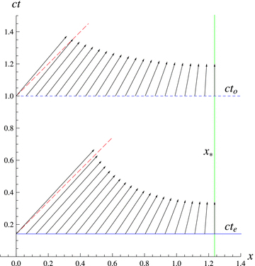
Parallel transport of the velocity four-vector of a distant galaxy, U, from the galaxy to the observer along the geodesic on the hypersurface of constant cosmic time. The transport is plotted for two values of time: the observation time, t_o (dashed horizontal line), and the emission time, t_e (solid horizontal line), both in units of t_o. The observer is in the origin of the coordinate system, x = 0, and the comoving coordinate of the emitting galaxy is x_* (vertical line) in units of c H⁻¹₀. The transportation is performed in comoving coordinates; in these coordinates all spatial components of the galaxy’s velocity four-vector are initially zero. During the transport towards the observer, the radial component of the four-velocity gradually increases. For better visibility and reasons explained in Section 5.2, in the plot this component is multiplied by a(t). Slanted long-dashed lines show the direction of null vectors at the events (t_o, 0) and (t_e, 0) in local inertial coordinates of the observer.

Open in new tabDownload slide

In practice, it is more interesting to know the recession velocity of a source at the time it emitted the photons which are reaching the observer today. In other words, the velocities at the time of emission are more interesting than the velocities at the time of observation. (There is even no guarantee that the emitting galaxy exists today.)

Combining equation (20) with (21) and (26), we obtain

47

Again, equation (47) assures that the recession velocity (at the time of emission) of a source with an arbitrarily high redshift is subluminal (v_e < c). In the empty (Milne) model, from (47) we obtain β_e = tanh [ln(1 +z)], or

48

in agreement with the Doppler formula. In the EdS model we obtain

49

In the currently favoured, flat model with non-zero Λ, equation (27) yields ⁠. The comoving distance is ⁠.

Let us now consider a source located at a redshift, e.g. 6. For the Milne model, the corresponding recession velocity at the time of emission, v^(M)_e, is 0.96c. For the EdS model, this velocity, v^(E)_e, is about 0.997c. For the flat model with Λ, adopting Ω_m = 0.24, the velocity, v^(Λ)_e equals approximately 0.991c. We interpret these values in the following way. A Milne universe is coasting, so v^(M)_e=v^(M)_o. An EdS universe decelerates, so it was expanding faster in the past. Therefore, it is logical that v^(E)_e > v^(M)_e.6 Similarly, one can also expect that v^(E)_e > v^(Λ)_e: in the flat Λ model, the assumed value of Ω_m is smaller than unity; moreover, there is a late-time phase of acceleration due to the cosmological constant. Interestingly, however, the value of v^(Λ)_e is greater than v^(M)_e and much closer to v^(E)_e. Apparently, for such a high redshift (and the adopted value Ω_m = 0.24), the effect of initial deceleration of the Universe on recession velocities strongly prevails over the opposing effect of its later acceleration. In fact this is not so surprising, since for Ω_m = 0.24 the flat model starts to accelerate only for a redshift as small as about 0.5.

On the other hand, for an arbitrarily high redshift there is always a range of sufficiently small values of Ω_m, for which v^(Λ)_e < v^(M)_e. We have checked that for Ω_m = 0.24, the critical redshift for which v^(Λ)_e=v^(M)_e is about 1.6.

6 DISCUSSION

Chodorowski (2007a) noted that in conformally flat coordinates in open, zero-Λ models, coordinate velocities of all galaxies are constant and subluminal. Lewis et al. (2007) pointed out that even in these coordinates, the proper velocities7 of sufficiently distant galaxies are superluminal. Lewis et al.’s (2007) criticism was fully justified, because coordinate velocities are meaningless. However, in this paper we have shown that the proper velocity is not a real velocity of a galaxy, so the fact that the former can be superluminal does not imply the same for the latter. Indeed, basing the definition of relative velocity given in this paper we have demonstrated that velocities of all particles of the cosmic substratum are in fact not superluminal.

In a recent paper, Faraoni (2010) studied the generation of the cosmological redshift by an instantaneous expansion of otherwise Minkowski space–time. A source and an observer were assumed to be at rest relative to each other both at the time of emission and observation of photons. It was also assumed that the universe expands only at a single instant of time t_X and t_e < t_X < t_o. Faraoni (2010) showed that the induced redshift is given by the canonical formula for all FLRW universes, 1 +z=a(t_o)/a(t_e). On the basis of this finding and the fact that the source and the observer were initially and finally at rest, he deduced that in the studied case the cosmological redshift is entirely gravitational. This is in agreement with our results, as will be explained below. Equations (20) and (21) are valid for any function a(t), not necessarily determined by the FL equations. The assumptions made by Faraoni imply that and from equation (21) one can see that, both at the time of emission and observation, the Dopplerian component of the cosmological redshift is zero. [Alternatively, from equation (20) it follows that the recession velocity vanishes.] However, Faraoni’s (2010) conclusion that the cosmological redshift is in general gravitational is incorrect. The quantity vanishes only for closed FLRW models and only for a single instant of time. More importantly, our Universe is certainly expanding now, and whatever the exact values of cosmological parameters, its expansion has been continuous in the past. Therefore, the cosmological redshift must be partly Dopplerian.

BH9 transported the four-velocity of a distant galaxy along the null geodesic connecting the source and the observer. [The original idea dates back to Synge (1960) and Narlikar (1994).] Instead, as the path of parallel transport we have chosen the geodesic connecting the source and the observer on the hypersurface of constant cosmic time. Both definitions are equally justified mathematically: both are intrinsic (i.e. they do not depend on any coordinate system) and reduce to the SR definition of relative velocity if the two observers are at the same point. The reason that as a path of transport we have chosen a geodesic on the hypersurface of constant cosmic time was to separate the effects of the curvature of the Universe from the effects of its evolution. We wanted to define the recession velocity at a well-specified instant of time. Transporting along a null geodesic provides v_BH, which is a sort of time-average (over the time interval between the times of emission and observation) of our, instantaneous recession velocity. Indeed, it can be easily verified that for small redshifts, hence also small time intervals, v_BH = (v_e+v_o)/2. As a consequence of their definition of relative velocity, BH9 found that in any FLRW cosmology and for any value of the redshift the cosmological redshift is related to the transported velocity v_BH by the relativistic Doppler formula.8 From this fact they deduced that the cosmological redshift is entirely Dopplerian. Our interpretation of the redshift is different: in a non-empty Universe there is gravitational field, inducing a gravitational shift. Therefore, with an exception of the empty model, the origin of the cosmological redshift must be partly gravitational. Using our definition of relative velocity, we have thoroughly proven this conjecture in the present paper. Thus, the difference between the findings of BH9 and ours is yet another hint that v_BH is not the recession velocity of a galaxy at a given instant of cosmic time. Using equations (37) and (41) it can be shown that for small redshifts, z = (β_e+β_o)/2 +[(β_e+β_o)/2]²/2. Comparing this equation with equation (41) we see that the relation between z and the effective velocity (β_e+β_o)/2 is indeed Dopplerian. But this effective velocity is just v_BH.

Different definitions of relative velocity lead to different interpretations of the cosmological redshift. However, the definition of BH9 and ours imply the same very important conclusion: recession velocities of all galaxies inside our particle horizon are subluminal. This fact is perhaps more fundamental than the specific value of recession velocity for a given redshift.

7 SUMMARY

In this paper we have decomposed the cosmological redshift into a Doppler shift and a ‘rest’, which we have interpreted as a gravitational shift. In order to extract the kinematic component from the cosmological redshift, we had to define properly the recession velocity of a distant galaxy. This velocity is a relative velocity of the galaxy and the observer, and in GR one cannot directly compare vectors at widely separated points. First, one has to transport parallelly the four-velocity of the distant galaxy to the observer. Next, the transported four-velocity is transformed to the local inertial coordinates of the observer and then the recession speed is typically extracted from the (transformed) radial component of the four-velocity. In general, parallel transport depends on the chosen path, but geodesics are special curves in GR and they seem to be a very natural choice for the problem under consideration. As the path, Synge (1960), Narlikar (1994) and BH9 adopted the null geodesic of photons emitted towards the observer. For reasons explained in Section 6, we have chosen a different path: the geodesic connecting the source with the observer on the hypersurface of constant cosmic time. BH9 found that in any FLRW cosmology and for any value of the redshift, the cosmological redshift is related to the transported velocity, as defined by them, v_BH, by the relativistic Doppler formula. From this fact they deduced that the cosmological redshift is entirely Dopplerian. However, from the PoE it follows that the cosmological redshift must be partly gravitational. The explanation of this apparent paradox is that v_BH is not a recession velocity at a specific instant of time, but rather a sort of an effective, time-averaged velocity.

In Section 3 we have presented analytical relations between the cosmological redshift and its Doppler component for two particularly simple cosmological models. In an empty universe, the cosmological redshift is entirely kinematic. This is expected, because in the empty model there is no gravitational field. In an Einstein–de Sitter universe, at the time of emission of photons the Doppler shift is greater than the total shift, so a gravitational shift is in fact a blueshift. At the time of observation, the situation is different: for large enough redshifts the gravitational component is dominant; in particular, even the particle horizon is receding with a speed smaller than that of light. This marked difference in the magnitude of kinematic components of the total redshift at the time of emission and at the time of observation is due to the fact that all matter-only models have expanded faster in the past.

Using only the PoE, in Section 4 we have independently decomposed the (non-relativistic) cosmological redshift into a Doppler shift and a ‘rest’, and have shown that in this regime the ‘rest’ is induced by the Newtonian gravitational potential. The obtained result is in agreement with a second-order expansion of the exact formula derived here in the framework of GR (Section 3), as well as with the classical formula of Bondi (1947) and equivalent findings of Peacock (1999) and Grøn & Elgarøy (2007).

Last but not the least, in Section 5 we have critically revised a widespread opinion that the recession velocities of (sufficiently) distant galaxies are superluminal. We have demonstrated that the commonly used proper velocity is not a recession velocity, but merely a radial component of the galaxy’s velocity four-vector (when expressed in proper coordinates). As such, it can indeed attain superluminal values. On the contrary, the definition of the recession velocity, presented in this paper, naturally implies that the velocity is subluminal for any value of the galaxy’s redshift. The definition of BH9 implies exactly the same conclusion. Basing our definition we have also argued that the expansion of the Universe is subluminal even on superhorizon scales. We plan to study this issue more comprehensively in a future work.

This work was partially supported by the Polish Ministry of Science and Higher Education under grant N N203 0253 33, allocated for the period 2007–2010.

REFERENCES