


Abstract
With the launch of the NASA Kepler spacecraft, the number of solar-like stars for which there are high-precision photometric observations available has increased considerably. In order to analyse the data from a large number of stars in a reasonable amount of time, automated pipelines are desirable. Here we present an extension of the OCTAVE (Birmingham–Sheffield Hallam) pipeline, which has been developed as part of the AsteroFLAG collaboration. While the first parts of the pipeline extracted overall oscillation parameters of the stars, here we present a significant extension to that pipeline designed in order to extract individual mode frequencies and amplitudes. The pipeline also attempts to label the detected modes by straightening and then identifying the ridges within the echelle diagrams in an automated manner. Tests have been performed on artificial stars and the pipeline is shown to return estimates of the mode frequencies that are in line with the input parameters. There does appear to be some positive bias in the returned value of the mode amplitudes which must be accounted for when employing the pipeline for real data.
1 INTRODUCTION
The Sun and other solar-like stars undergo acoustic oscillations which are the visible manifestation of trapped acoustic standing waves that propagate within their subsurface convection zones. These modes travel to different depths within the stellar interiors and hence the analysis of the parameters of these oscillations, known as asteroseismology, is a very powerful tool in helping to determine the dynamics and characteristics of the stellar structures as a function of depth.
Unfortunately these types of acoustic oscillations have relatively small amplitudes which make observing them on stars other than the Sun very challenging. Even so, over the past decade or so a number of studies have been successful in detecting acoustic oscillations on other stars. These include both ground-based observations which take mainly Doppler-velocity measurements using spectrographs, e.g. ELODIE (Baranne et al. 1996), CORALIE, HARPS (Queloz et al. 2001), UCLES and UVES (D'Odorico 2000), and space-borne instruments that use photometric techniques such as WIRE (Buzasi et al. 2000), MOST (Matthews et al. 2000) and most recently CoRoT (Baglin et al. 2006). For a recent pre-CoRoT review of some of these programmes see Bedding & Kjeldsen (2008). Some CoRoT results are presented in Michel et al. (2008) and Appourchaux et al. (2008).
The successful launch of the NASA Kepler satellite on 2009 March 7 should considerably increase the number of stars with confirmed detections. For a detailed description of the Kepler mission design and review of the early science results, see Koch et al. (2010), Chaplin et al. (2010) and Gilliland et al. (2010). The main goal of the Kepler mission is to detect Earth-like exoplanets using the transit technique, and in order to accomplish this Kepler continuously monitors around 100 000 stars with magnitude of 16 or brighter. However, the photometric data collected are also very well suited to asteroseismology. It is expected that over the 3.5-yr lifetime of the Kepler mission, time series suitable for asteroseismology will be collected for over 1000 solar-like stars.
Because of this, it is clear that automated pipelines will be needed to analyse the data and return overall oscillation parameters and individual mode parameters. A number of these pipelines have either already been developed or are currently in development (see Hekker et al. 2009; Huber et al. 2009; Basu, Chaplin & Elsworth 2010; Campante et al. 2010; Karoff, Campante & Chaplin 2010; Mathur et al. 2010) as part of the AsteroFLAG collaboration (see Chaplin et al. 2008) and outside of it (see Mosser & Appourchaux 2009; Kallinger et al. 2010). Here we present an extension to the OCTAVE pipeline outlined in Hekker et al. (2009, hereafter referred to as Paper I). The initial part of the pipeline was mainly concerned with returning overall oscillation parameters such as the frequency range of oscillations, the frequency at which the maximum oscillation power occurs and the large and small frequency separations between consecutive radial orders. In this extension to the pipeline, we attempt to ‘peak-bag’ (a term common in the helioseismic and asteroseismic communities), i.e. to determine individual mode parameters such as the mode frequencies, amplitudes and linewidths. We do this by fitting a model to the power spectra. This method also gives better prospects of determining the small separation.
In this paper, we briefly outline the simulated data used to test the peak-bagging pipeline before going on to describe the methodology in Section 3. In Section 4 we compare the results of peak-bagging with those of the input parameters used to create the artificial data. The results are discussed and summarized in Section 5.
2 SIMULATED DATA
The simulated time series used here are the same as in Paper I and are based on stellar parameters from the Kepler Input Catalogue (KIC; see Latham et al. 2005). A range around each KIC value was determined from expected formal and systematic errors and values were chosen at random from this range. These values were used as inputs to the model grid prepared for the Aarhus Kepler pipeline (see Quirion, Christensen-Dalsgaard & Arentoft 2010). Time series were then generated using the mode parameters determined from the model grid. Rotation effects, granulation, activity and white noise appropriate to the brightness of the target have all been included in the data sets. Additionally, the lifetimes of each of the oscillation modes have been varied.
The stellar models were generated using astec (Aarhus stellar evolution code; Christensen-Dalsgaard 2008a). The OPAL equation of state was employed along with the solar mixtures of Grevesse & Noels (1993) using the OPAL and Alexander & Ferguson (1994) opacity tables. The p modes frequencies were calculated using adipls (Aarhus adiabatic pulsation code; Christensen-Dalsgaard 2008b).
Each of the time series were 30-d long and had a 1-min cadence in order to match the observing characteristics of the first Kepler data. In total 353 artificial stars were simulated, but the values of the input data were only released for half of the stars. Hence, we have been able to test the results of the pipeline on 177 data sets.
3 METHODOLOGY
The aim of extending the OCTAVE pipeline was to perform an automated peak-bagging process on the power spectra of stars observed by the Kepler instrument. It was hoped that in fitting the modes via a standard peak-bagging analysis, we could better constrain the estimates of the following parameters:
individual frequencies;
average-mode linewidths (hence mode lifetimes);
average-mode amplitudes;
and also obtain estimates of
individual mode amplitudes,
average small separation between ℓ = 0 and 2 modes.
The peak-finding and peak-fitting methods are described below. We also describe an automated method for mode identification which is needed to determine the small separation of the oscillations. However, the manner in which we perform the fitting is such that we do not first need to identify the angular degree of the modes. Indeed correct identification of the modes is only possible on a minority of the artificial stars (around 30 per cent).
3.1 Peak finding
The initial part of the OCTAVE pipeline returns individual mode frequencies using a Bayesian approach. The method is based on determining whether peaks in the power spectrum are more likely to be the result of a true signal (H1 hypothesis) or just due to noise (H0 hypothesis).
However, here we determine the mode frequencies separately using a frequentist approach. In this case, only the probability that a peak is due to noise is considered. Hence, any peak that has a very low probability of being due purely to noise is taken to be a candidate mode.
Even though the time series being investigated here are only 30 d long and as such the resolution of the power spectra is just 0.39 μHz per bin, the power within individual modes may still not fall within a single frequency bin. This could be due to a large linewidth or in the case of the ℓ = 1 and 2 modes, a large rotational splitting (assuming the inclination is also well above zero). Therefore, in order to account for this, we smooth each spectrum over a range of five bins (∼2 μHz) before carrying out the probability test.
The fact that we are averaging over a number of bins affects the probability calculation. However, it can be shown that the probability of having a power, s, averaged over Mav bins for a χ2 distribution with D degrees of freedom is equivalent to finding the probability of having power, s, in a single bin for a χ2 distribution with DMav degrees of freedom (see Appourchaux 2004).
A value of P close to unity indicates a high probability that the power in that bin is not due solely to noise. We therefore tag all frequency bins with P≥ 0.9 as possible mode detections. In the case where we have a single isolated bin that passes the threshold, we could simply tag that detection with the corresponding frequency. However, it is far more common to obtain a number of bins within a small range of each other, all of which have P≥ 0.9 but which all correspond to a single mode. In order to deal with this, we smooth each spectrum a further three times (we refer to this as the ‘heavily’ smoothed spectrum). This has the effect of averaging most of the stochastic nature of the spectrum without drastically reducing the overall resolution. We can then take the maxima in the heavily smoothed spectrum and check to see if there was a spike in power that passed the probability test within 1 μHz either side of that peak in the unsmoothed spectrum. If there was, we tag it as a mode with a frequency equal to that of the peak in the heavily smoothed spectrum.
3.2 Fitting
It is common practice to attempt to identify the angular degrees of the visible modes before any attempt is made to fit them. This is because modes with different ℓ have different rotational splitting patterns. However, when dealing with short data sets that have poorly resolved spectra, unless the star is rotating relatively rapidly and has a large inclination, it is difficult to detect more than a single peak associated with each mode.
For this reason, we employ a strategy that fits only a single Lorentzian model to each detected peak. Hence we are ignoring any effect of the splitting and inclination. The likely result of this would be to fit a slightly increased linewidth. However, in a very few cases, the rotational splitting may be large enough that more than one peak will be identified by the peak-finding algorithm.
The model was fitted to the power spectrum by maximizing an appropriate log-likelihood function using a Powell multidimensional hill-climbing minimization algorithm (i.e. the POWELL routine in idl). The function used is based on the assumption that the power spectrum is distributed with negative exponential (i.e. χ2, with two degrees of freedom) statistics (see Anderson, Duvall & Jefferies 1990). Note that we actually fit the log of the heights, linewidths and background as opposed to the linear values. This is because the logs of these values more closely follow Gaussian distributions than their corresponding linear values and hence the formal uncertainties can be determined more accurately from the inverse Hessian matrix.
Although this is a very simple fitting model, as suited to the short lengths of the time series that will be initially available from the Kepler mission, it should be noted that the code developed here is highly customizable and can easily be modified to allow for more complicated models when dealing with longer time series.
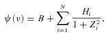
3.3 Mode identification
Once the frequencies have been fitted, an attempt is made to identify the modes in an automated manner (i.e. correctly label the angular degree, ℓ and radial order, n). To visualize the approach taken, it is useful to consider an echelle diagram (see Grec, Fossat & Pomerantz 1983) in which the frequency spectrum is divided into slices of length equal to the large separation. The reduced frequencies (the actual frequencies minus the starting frequency of each slice) are then plotted against the starting frequency of each slice. This process is akin to stacking the frequency slices on top of each other. According to the asymptotic expression for acoustic modes (Tassoul 1980), one would expect the modes of the same ℓ to lie directly above each other in distinct ridges. However, certain physical characteristics of the stellar interiors can lead to echelle diagrams of real stars (and indeed the Sun) having kinks and curves in the ridges. Fig. 1 shows the echelle diagram of one of the artificial stars where three distinct ridges can be seen.
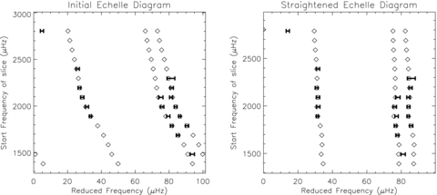
Example of an echelle diagram for the artificial star 10963065. The error bars show 3σ below the frequency of the fitted peak to 3σ above, while the diamonds give the actual frequency inputs. Three distinct ridges can be seen showing the ℓ = 0, 1 and 2 modes. The left-hand panel shows the initial echelle diagram, while the right-hand panel shows a ‘straightened’ echelle diagram (see Section 3.3.1).
3.3.1 Ridge straightening
The curvature of the ridges can make it difficult for an automated procedure to correctly identify the modes. Therefore the first step in our identification process is to ‘straighten’ the ridges. This is done by adjusting three parameters, the large separation, Δν, a curvature factor, c, and the order of the slice at which the curvature factor operates from, n0. A value for Δν is already returned from the initial part of the OCTAVE pipeline, and this provides a useful starting parameter for the above optimization process. However, if the echelle diagram shows that the ridges are slanted as opposed to vertical, then it suggests that the Δν may need to be adjusted slightly. Also, to remove as much of the curvature in the ridges as possible, the quantity c * δn is added to each frequency where δn is the number of slices a particular peak is away from the n0 slice. The straightening is achieved using the following optimization procedure.
The echelle diagram is split in two at the mid-point on the x-axis (i.e. half the large separation).
The mean frequency of all the peaks in the lower reduced frequency half is calculated.
Any peaks whose frequencies lie outside a given tolerance of the mean are removed from the calculation.
The standard deviation of the remaining frequencies is calculated.
The three parameters, Δν, c and n0, are adjusted using a Powell hill-climbing optimization process until the standard deviation is minimized.
The procedure is repeated for the peaks in the other half of the echelle diagram.
The final parameter results from the half which gave the lowest standard deviation are applied to the entire echelle diagram.
An example of one particular echelle diagram before and after applying the straightening procedure is given in Fig. 1.
3.3.2 Ridge location
The second part of the process tries to locate the ridges within the echelle diagram. This is done by grouping together peaks which have similar reduced frequencies once the straightening procedure has been applied. The specific steps to achieve this are the following.
Find the strongest fitted peak and store its frequency.
Move up to the next slice within the echelle diagram and check if the peak whose reduced frequency is closest to the last stored peak is within a given tolerance. If it is, store that frequency. If it is not (or there is no fitted peak at all), then move up to next slice and repeat the process. The best value to set the tolerance at was found to be 4 μHz.
Repeat this procedure until there are three slices in a row where no matching peak is found or until the highest frequency slice is reached.
Repeat steps (ii) and (iii) but move down in frequency from the strongest fitted peak.
Find the strongest peak of those not yet tagged and store its frequency.
Repeat steps (ii) through (v).
Repeat the entire process until all the fitted peaks have been stored in this manner.
Tests on the artificial stars seem to show that this procedure is relatively robust for stars where a reasonable number of modes have been found (e.g. at least eight or more) and which have modes with relatively high frequencies (i.e. greater than ∼800 μHz). Stars with modes below this frequency are more likely to have a high number of ‘mixed’ modes. This results in a number of modes not falling in the expected ridges and hence throws off the ridge location procedure. Other problems that can affect this procedure are the presence of too many false positive mode detections, large rotational splitting and a small value of the small separation.
3.3.3 Ridge identification
The final part of the procedure determines which set of modes should be tagged with which value of ℓ. If three or more ridges have been found (i.e. there are three sets of peaks that have at least two peaks within them), then we identify according to this process:
find the three sets of peaks (ridges) that have the largest combined power;
find the mean reduced frequency of each of these ridges;
label the ridges that have the closest mean reduced frequency as ℓ = 2 and 0 (with the lower value being labelled 2 and the higher 0);
label the remaining ridge as ℓ = 1.
If only two ridges are identified, then there are two possibilities as to why this might be. On the one hand it may be that the small separation is of the order of or less than the mode linewidth, in which case the ℓ = 0 and 2 ridges cannot be distinguished separately. Or it may be that the ℓ = 0 and 2 ridges are well separated but the signal-to-noise ratio is low and hence many of the weaker ℓ = 2 modes have not been clearly detected. In the first case, we would expect that the average power per mode in the ridges to be the same (see Ballot 2010 for a mathematical demonstration). However, in the second case, where we would be comparing an ℓ = 0 ridge with an ℓ = 1 ridge, we would expect the power per mode to be greater in the ℓ = 1 ridge (e.g. see Bedding et al. 1996; Kjeldsen et al. 2008). This can be used as a possible method of identifying the modes, and therefore in cases where only two ridges are detected, we employ the following procedure.
Find the average power per mode for the two ridges.
Label the ridge with the highest power per mode as ℓ = 1.
Label the ridge with the lowest power per mode as ℓ = 0.
This method will obviously not be robust in cases where the ℓ = 0 and 2 ridges cannot be distinguished separately. Therefore, we also check to see how significant the difference in the average power per mode is for the two ridges. We make the assumption that the larger the difference, the more likely it is we are comparing a distinct ℓ = 0 and 1 ridge and thus the more confident we can be in our mode identification.
One advantage of the mode-identification procedure is that it will remove many of the false positive mode detections. There is also the possibility that mixed modes will be removed as they tend to fall outside the expected ridges. However, such modes can be included in the final list of frequencies for the star, without a degree label.
4 RESULTS
Of the 177 artificial stars that we had known input data for, 102 had at least one mode detected. However, we give results only on the 78 (44.4 per cent) artificial stars where five or more modes were found. In the remainder of this section, we go on to discuss how well the mode-finding routine worked in terms of the number of modes found and the number of false detections. We also show how accurate the estimates of the mode frequencies, amplitudes and linewidths returned from the peak-bagging process were.
4.1 Frequencies
The central frequency is the most robust of the mode parameters. As long as the peak is strong enough to be confidently detected above the background noise, it is a relatively straightforward task to estimate that mode's frequency. The main complications occur when fitting the non-radial modes (ℓ≠ 0), as the effect of rotational splitting means that these modes will manifest as a multiplet. However, whether these peaks can be resolved as separate peaks or not will depend on the time series length, the size of the rotational splitting, the linewidth and the star's inclination.
We compare the fitted frequencies with the known input values. If a frequency estimate occurs within 2 μHz of an actual input frequency and that input peak has a signal-to-noise ratio of greater than unity, then we take that as a positive detection. If these conditions are not met, we assume the fitted peak is a false detection. In the case of non-radial modes, things are a little more complicated as we can either define the input frequency as the central (m = 0) value or take the frequencies of the individual m components. We choose to employ both cases and refer to the first as Case A and the second as Case B.
For the 78 stars where at least five modes were found, a total of 960 modes passed the probability test. Of these, 131 (13.6 per cent) were defined to be false detections by Case A and 117 (12.2 per cent) by Case B. For the positive mode detections, we can analyse the distribution of the fitted frequencies about the input values. This is shown in Fig. 2 where we have plotted histograms of the fits about the input values as a function of the formal error. We show the results for ℓ = 0, 1 and 2 modes on separate panels.
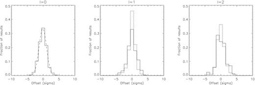
Histrograms showing the distribution of the offset of the fitted frequencies compared with the input frequencies divided by the formal uncertainty. The solid lines give the Case A results, while the dotted line gives the case B results. The dashed curve overlaid in the ℓ = 0 plot shows the fitted Gaussian.
The results may be summarized as shown in Table 1, where we show the percentage of fits falling within 1σ, 2σ, 3σ and 5σ for each ℓ and for each input comparison case. In most cases, we would expect the results for the radial modes to be the most robust because there is no complication due to multiple components. However, if the small separation is small, then the fitted frequencies of the ℓ = 0 modes may be affected by the presence of undetected ℓ = 2 modes. While the percentages falling within the given σ limits are less than we would expect in a purely Gaussian case, they are better constrained than the frequency estimates determined in Paper I which, for ℓ = 0 modes, found only 77 per cent of the estimates falling within 3σ of the input value, compared with 93 per cent shown in Table 1. The percentage of fits falling within each σ limit for the ℓ = 1 and 2 modes in Case A are somewhat lower than for ℓ = 0. In contrast, Case B seems to give very good agreement across all three ℓ values within the 2σ, 3σ and 5σ ranges although ℓ = 1 and 2 seem to give a higher fraction of fits within the 1σ range than we see for ℓ = 0.
Fraction of fitted frequencies within certain ranges of the input values as a function of the formal uncertainty. The ℓ = 1 and 2 values given in columns 3 and 4 give the Case A results and those in columns 5 and 6 give the Case B results.
| σ | ℓ = 0 | ℓ = 1 | ℓ = 2 | ℓ = 1 | ℓ = 2 |
| 1 | 0.53 | 0.50 | 0.50 | 0.68 | 0.64 |
| 2 | 0.84 | 0.75 | 0.73 | 0.84 | 0.89 |
| 3 | 0.93 | 0.86 | 0.86 | 0.93 | 0.95 |
| 5 | 0.99 | 0.96 | 0.97 | 0.97 | 0.99 |
| σ | ℓ = 0 | ℓ = 1 | ℓ = 2 | ℓ = 1 | ℓ = 2 |
| 1 | 0.53 | 0.50 | 0.50 | 0.68 | 0.64 |
| 2 | 0.84 | 0.75 | 0.73 | 0.84 | 0.89 |
| 3 | 0.93 | 0.86 | 0.86 | 0.93 | 0.95 |
| 5 | 0.99 | 0.96 | 0.97 | 0.97 | 0.99 |
These results can be explained by the fact that we may not always fit the entire rotationally split mode, but instead might fit only a single component. This could occur when the splitting and inclination are both high, but one component is damped while the other is stochastically enhanced. In this instance, comparing the fit with the central frequency will give a larger offset than if we compare with the correct m component. Hence, in Case A the fraction of fits falling within a certain range of the input central frequency is lower for ℓ = 1 and 2 than for ℓ = 0. Conversely, it is also possible that when comparing the fitted frequencies with the input frequencies of the components, we actually make a comparison with the wrong peak. This can occur because we have up to three frequencies to test against in the ℓ = 1 case and up to five in the ℓ = 2 case. It is likely that the fitted peak will fall in close proximity to at least one of these values and hence artificially reduce the offset. Hence, in Case B, we see a larger fraction of correct fits within the given σ ranges.
The fact that a lower fraction of fits fall within the expected Gaussian σ ranges suggests that we need to revise upwards the estimates of the formal uncertainties on the frequencies. The fitted Gaussian curve shown in the ℓ = 0 panel of Fig. 2, has a normalized width of 1.3 which indicates our uncertainties underestimate the true values by about 30 per cent. However, if we look at the ℓ = 0 frequency fits as a function of frequency, as shown in Fig. 3, we can see that the offset is greater for those stars which have frequencies below around 2500 μHz. To investigate this further we plot, in Fig. 4, separate histograms of the distributions for those frequency fits below 2500 μHz and those above. Gaussian curves fitted to these distribution have widths of 1.42 in the low-frequency case and 0.96 for high frequencies. This suggests that the formal uncertainties on modes with frequencies below 2500 μHz should be multiplied by a correction factor of around 1.4, while the uncertainties on modes fitted above this frequency should be taken as given.
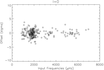
Offset between fitted and input frequencies divided by the formal uncertainty for ℓ = 0 modes as a function of input frequency.
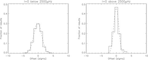
Histograms showing the distribution of the offsets of the fitted frequencies compared with the input frequencies divided by the formal uncertainty for the ℓ = 0 modes. The distribution of modes with frequencies below 2500 μHz are shown in the left-hand panel and those above in the right-hand panel. The dotted line shows fitted Gaussian curves.
The increased spread in the fitted values at low frequencies is likely due to a problem in the mode-finding algorithm. Determining the probability that a peak is due to noise depends on the background. Hence, uncertainties in the background can lead to larger uncertainties in the extraction of individual mode parameters and the uncertainties on the background tend to be higher for stars that have modes at lower frequencies.
4.2 Amplitudes
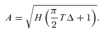
In Fig. 5, we plot the calculated amplitudes against the corresponding input values for each ℓ. We have also plotted the expected one-to-one relationship. The plot shows that the fits follow the general trend of this relationship, but there is clearly a systematic positive bias. This bias is stronger for the ℓ = 1 and 2 modes than it is for ℓ = 0.
Fitted amplitudes plotted against the input amplitudes for individual ℓ. The one-to-one relationship is shown by the bold line.
This bias is not unexpected. It has been shown before that when the time series is short and/or the signal-to-noise ratio of the peaks is low, a traditional fitting method such as this can often return overestimated heights and underestimated linewidths (Fletcher et al. 2006; Fletcher 2007). As mentioned above, this effect will be somewhat compensated for when calculating the amplitudes. However, in this instance we are fitting individual heights to the modes but only a single average linewidth across all the modes. Therefore, the underestimate in the linewidths is likely to be smaller than the average overestimate in the heights.
The larger bias in the ℓ = 1 and 2 modes is a result of both not fitting a rotational splitting and fitting a single average linewidth. Fitting a single peak to a rotationally split mode will result in a larger linewidth being fitted. However, since we also fit the ℓ = 0 modes with the same linewidth, the model cannot account fully for the presence of multiple peaks by fitting a larger linewidth, hence it will attempt to compensate by increasing the heights, which ultimately increases the amplitudes. This effect is even greater for the ℓ = 2 modes, hence we see an even greater bias in the determined amplitudes compared with the inputs. In order to account for the overestimation, the fits to the artificial data show that the determined amplitudes should be decreased by ∼10 per cent for the ℓ = 0 modes, ∼30 per cent for ℓ = 1 and ∼50 per cent for ℓ = 2.
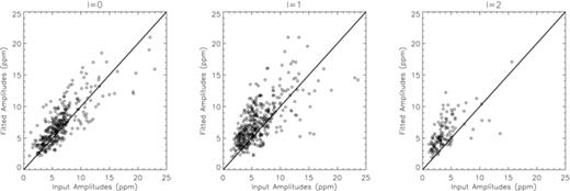
4.3 Linewidths
The initial part of the OCTAVE pipeline (see Paper I) produces estimates for the average linewidth (or equivalently the damping time) of the most prominent modes. This was done by attempting to calculate the average height and power of each mode in order to extract the mode width. Here we simply fit for an average linewidth across all detected modes. The advantage of this method is that we do not need prior estimates of either the mode power or height to obtain the linewidth. However, it should be noted that the fitted heights and widths are strongly correlated as discussed in Section 4.2.
The results of fitting the average widths are shown in Fig. 6. The fits are plotted as a function of temperature and the input values which follow the relationship of Δ∝T4eff are shown by the dotted line. Again, we have only plotted those stars where at least five modes were detected and fitted. It can clearly be seen that the linewidths follow the input relationship quite well given the errors. Comparing this plot with that of fig. 4 in Paper I shows that the fitting method described here returns significantly better constrained estimates of the average linewidth. This can be confirmed by taking the standard deviation of the average linewidths about the input values. For the same set of stars, this was found to be 0.55 μHz using the method in Paper I, compared with a value of 0.43 μHz found here.
Fitted linewidths plotted as a function of effective temperature. The  input relationship is shown by the dotted line.
4.4 Mode identification and small spacings
In this section, we look at the results of the mode-identification procedure outlined in Section 3.3. While not perfect, the process does seem to be robust for stars that have a relatively high number of modes detected and very few mixed modes. Because of this, we only report the results of those stars where at least eight modes were detected and which had modes detected only above 800 μHz. Of the 177 stars we had input data for, 54 matched these criteria. Of those 54, the mode-identification procedure correctly identified the modes in 48 cases. For 35 of the stars ℓ = 2 modes were detected and identified. The presence of an ℓ = 2 ridge makes the mode-identification procedure far more robust and in all but one case, the modes were identified correctly. Without the ℓ = 2 modes, we make the assumption that the average height of the ℓ = 1 modes will be greater than that of the ℓ = 0 modes and use this to make the identification. Of the 19 stars where no ℓ = 2 modes were detected, the modes were labelled correctly on 14 occasions using this method. On two out of the five cases where this method failed, it was due to the small separation being small enough that the ℓ = 0 and 2 modes were detected as a single mode and hence fitted as such. It was found that in the large majority of cases, the reason no ℓ = 2 ridge was detected was due to the weakness of the ℓ = 2 modes.
One big advantage of the mode-identification procedure is that many of the false positive detections are thrown out. For the 54 stars where we attempt to identify modes, a total of 646 modes were identified. Of these, 61 (9.4 per cent) were defined to be false detections by Case A and 41 (6.3 per cent) by Case B. Thus we reduce the number of false detections by about half when we are able to identify the modes (see Section 4.1).
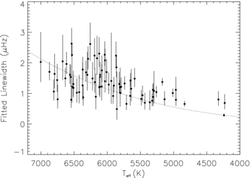
If three separate ridges can be seen in the echelle diagram, it is also possible to determine the average small separation. This determination is made by taking the difference between the mean reduced frequencies of the fitted ℓ = 0 and 2 modes from the straightened echelle plot. The errors are then taken to be the combined error as determined from the scatter of the fitted modes about the mean in the two ridges. We can compare this with the average small separation determined from the input values as shown in Fig. 7. Note that the input small spacings have been calculated from the same modes that were detected from the pipeline so as to provide a meaningful comparison. The fitted values follow the one-to-one relationship of the input values reasonably well given the errors. The few values that seem to be outliers are mainly due to false detections biasing the result.
Average fitted versus input small separations. The one-to-one relationship is shown by the straight line.
5 SUMMARY
We have developed extensions to the OCTAVE (Birmingham–Sheffield Hallam) pipeline which include a peak-bagging routine in order to determine individual mode parameters of the stars such as mode frequencies and amplitudes and a mode-identification routine designed to tag the modes with their correct angular degree. We have tested the peak-bagging procedure on the same set of artificial stars that the initial pipeline (see Paper I) was tested on and find that some level of peak-bagging could be performed on around half of the stars. This compares with the results in Paper I which found that estimates of the large separation could be returned for around three quarters of the stars. By comparing the fitted parameters with the known input parameters, the following conclusions can be made.
The fitted frequencies match the input frequencies well with around 90 per cent of the estimates falling within 3σ of the input values (see Table 1).
The spread in the fitted values about the input values is larger for high-mass stars with low-frequency modes (<2500 μHz). This suggests the formal errors reported on the fitted frequencies for similar high-mass real stars should be increased by around 40 per cent.
The fitted amplitudes overestimate the input amplitudes by a significant amount. The amount of overestimation increases for modes with higher ℓ, around 10 per cent for ℓ = 0, 30 per cent for ℓ = 1 and 50 per cent for ℓ = 2.
The fitted average linewidths match the input values well, and the standard deviation in the fitted linewidths is significantly lower than the linewidths determined in the first part of the OCTAVE pipeline.
The automated mode identification routine is applied after the modes have been fitted. This procedure utilizes newly designed ridge straightening and subsequent ridge identification routines. The procedure seems relatively robust for stars that have at least eight detected modes with frequencies above around 800 μHz. Stars with detected modes which had frequencies below this value often have a number of mixed modes which can cause problems for the automated mode-identification procedure. The procedure is very successful (97 per cent of the cases) when an ℓ = 2 mode ridge can be detected and while less good, is still relatively successful (74 per cent of the cases) when this is not the case.
We thank the Science and Technology Facilities Council (STFC) for their support. We are also grateful for the support of the AsteroFLAG group whose workshop programme is funded by the International Space Science Institute (ISSI).
REFERENCES
