


Abstract
Period–luminosity relations (PLRs) of type II Cepheids (T2Cs) in the Small Magellanic Cloud (SMC) are derived based on OGLE-III, IRSF/SIRIUS and other data, and these are compared with results for the Large Magellanic Cloud (LMC) and Galactic globular clusters. Evidence is found for a change of the PLR slopes from system to system. Treating the longer period T2Cs (W Vir stars) separately gives an SMC–LMC modulus difference of 0.39 ± 0.05 mag without any metallicity corrections being applied. This agrees well with the difference in moduli based on different distance indicators, in particular the PLRs of classical Cepheids. The shorter period T2Cs (BL Her stars) give a smaller SMC–LMC difference suggesting that their absolute magnitudes might be affected either by metallicity or by age effects. It is shown that the frequency distribution of T2C periods also changes from system to system.
1 INTRODUCTION
Cepheids are pulsating stars with periods between 1 d and about 100 d. Although there was originally some confusion, see the review by Fernie (1969), it is now believed that Cepheids can be grouped into two distinct classes: classical Cepheids and type II Cepheids (T2Cs, hereafter). The former are intermediate mass stars (4–10 M⊙), while the latters are lower mass stars (∼1 M⊙) belonging to disc and halo populations (Wallerstein 2002; Sandage & Tammann 2006).
T2Cs are conventionally divided into three period groups, BL Her stars (henceforth BL) at short periods, W Vir stars (WV) at intermediate periods and RV Tau stars (RV) at the longest periods. According to Gingold (1976, 1985), the BLs are stars evolving from the horizontal branch to the Asymptotic Giant Branch (AGB); the WVs are stars that along the AGB cross the Cepheid instability strip due to excursions towards higher effective temperatures; the RVs are stars that after their AGB phase are moving towards the white dwarf cooling sequence. However, some later evolutionary tracks (e.g. Pietrinferni et al. 2006) do not show the excursions, and the precise evolution state of T2Cs remains unclear. We follow the division by Soszyński et al. (2008b) and adopt thresholds of 4 and 20 d to divide the three groups. The RV stars tend to show alternating deep and shallow minima (and this is often taken as a defining characteristic), but the single period of the RVs will be used in this paper. In addition to these three groups, Soszyński et al. (2008b) established a new group of T2Cs, peculiar W Vir (pW) stars. They have distinctive light curves and tend to be brighter than normal T2Cs of the same period. It is suggested that many, perhaps all, of them are binaries, but their nature remains uncertain. The bright Galactic T2C κ Pav appears to be a pW star (Matsunaga, Feast & Menzies 2009, hereafter M09).
Matsunaga et al. (2006, hereafter M06) discovered a tight PLR of T2Cs in globular clusters based on infrared (IR) photometry for 46 T2Cs. Feast et al. (2008) used pulsation parallaxes of nearby T2Cs to calibrate this cluster PLR and to discuss the distances of the Large Magellanic Cloud (LMC) and the Galactic Centre. The Optical Gravitational Lensing Experiment (OGLE-III) have significantly increased samples of T2Cs in the Magellanic Clouds. Soszyński et al. (2008b) found 197 T2Cs in the LMC. M09 investigated their (near-IR) nature and confirmed that BL and WV stars follow a tight PLR like that of T2Cs in globular clusters, whereas RV and pW stars show a large scatter and are systematically brighter than the PLR for the BL and WVs. The calibration by Feast et al. (2008) then leads to a distance modulus of the LMC of 18.46 ± 0.05 mag. These investigations have established the T2Cs as a promising distance indicator.
The aim of the present paper is to compare the T2C PLRs in the Small Magellanic Cloud (SMC), LMC and globular clusters. This is important for a further study of these relations and their possible dependence on metallicity and other factors. The OGLE-III survey discovered 43 T2Cs in the SMC (Soszyński et al. 2010b, S10 hereafter). In the following, we first collect near-IR JHK magnitudes of SMC T2Cs (Section 2) and investigate their PLRs (Section 3). The reddening-free PLR in VI is also discussed. In parallel with our work, Ciechanowska et al. (2010, C10) have obtained independent J and K for a subset of the SMC T2Cs and their data are combined with ours in some of the discussions. We find evidence that the BL and WV stars need to be discussed independently. In Section 4 the apparent differences in distance moduli of the LMC and SMC are derived for these stars and compared with the differences obtained from other objects. The data used for classical Cepheids are discussed in an appendix. In addition, the colours and period distributions of T2Cs in various systems are compared and contrasted in Sections 5. Section 6 summarizes the present work.
2 INFRARED PHOTOMETRY
S10 catalogued 43 T2Cs in the SMC: 17 BLs, 10 WVs, seven pWs and nine RVs. We searched for near-IR counterparts of these stars in the catalogue of Kato et al. (2007). This point-source catalogue is based on simultaneous images in JHKs obtained with the 1.4-m Infrared Survey Facility (IRSF) located at South African Astronomical Observatory (SAAO), Sutherland, South Africa. The catalogue covers 40 deg2 of the LMC, 11 deg2 of the SMC and 4 deg2 of the Magellanic Bridge. The catalogue extends to fainter magnitudes and has higher resolution than the point-source catalogue of the Two-Micron All-Sky Survey (2MASS; Skrutskie et al. 2006) in the regions of the Magellanic Clouds. The 10σ limiting magnitudes of the survey in the SMC are 18.9, 17.9 and 16.9 mag for J, H and Ks. These limits are fainter than those for the LMC since the crowding effect is less (Kato et al. 2007).
Matches between the OGLE-III and IRSF catalogues were found for 39 S10 T2C sources with a tolerance of 0.5 arcsec (Table 1). The differences in coordinates are small between the catalogues with standard deviations of less than 0.1 arcsec in both Right Ascension (RA) and Declination (Dec.). Four OGLE-III sources (IDs in S10: #5, #37, #42 and #43) are located outside the IRSF survey field. In the case of two matched objects, #6 and #22, Ks-band magnitudes are missing because of the faintness of these stars, both of which are BL stars with relatively short periods (P < 1.5 d). Although about half of the BL sample have Ks fainter than the 10σ limiting magnitude, their J and H magnitudes are brighter than the limits.
The catalogue of OGLE-III T2Cs in the SMC with IRSF counterparts. Modified Julian Dates (MJD), pulsation phase of the observations, JHKs magnitudes and their errors are listed for each IRSF measurement as well as the OGLE-IDs, types and periods. Shifts for the phase corrections (δφ) obtained from the I-band light curves are also listed. Two sources, #28 and #35, are listed twice because they are located in overlapping fields of the IRSF survey.
| OGLE-ID | Type | log P | IRSF counterpart | δφ | ||||||||
| IRSF-Field | MJD(obs) | Phase | J | EJ | H | EH | Ks | EKs | ||||
| 1 | pWVir | 1.07441 | SMC0031-7350F | 52847.100 | 0.944 | 14.32 | 0.01 | 14.01 | 0.01 | 14.00 | 0.01 | 0.076 |
| 2 | BLHer | 0.13741 | SMC0037-7250C | 52518.027 | 0.115 | 17.84 | 0.04 | 17.56 | 0.08 | 17.65 | 0.14 | 0.145 |
| 3 | WVir | 0.63947 | SMC0036-7350G | 52849.096 | 0.677 | 17.27 | 0.03 | 16.95 | 0.04 | 17.06 | 0.14 | −0.160 |
| 4 | WVir | 0.81514 | SMC0037-7310A | 52517.858 | 0.911 | 16.16 | 0.04 | 15.80 | 0.04 | 15.69 | 0.05 | 0.025 |
| 6 | BLHer | 0.09188 | SMC0041-7330A | 52494.999 | 0.263 | 18.06 | 0.05 | 17.93 | 0.11 | – | – | 0.094 |
| 7 | RVTau | 1.49081 | SMC0041-7310D | 52496.056 | 0.372 | 13.10 | 0.01 | 12.74 | 0.01 | 12.62 | 0.02 | −0.090 |
| 8 | BLHer | 0.17312 | SMC0046-7330I | 53413.759 | 0.552 | 17.60 | 0.05 | 17.03 | 0.06 | 17.05 | 0.24 | −0.086 |
| 9 | BLHer | 0.47291 | SMC0046-7250C | 52457.193 | 0.867 | 17.17 | 0.03 | 16.81 | 0.03 | 16.73 | 0.07 | 0.118 |
| 10 | pWVir | 1.24256 | SMC0046-7330E | 53301.789 | 0.454 | 13.83 | 0.02 | 13.52 | 0.02 | 13.45 | 0.02 | −0.025 |
| 11 | pWVir | 0.99675 | SMC0046-7330E | 53301.789 | 0.451 | 14.34 | 0.01 | 14.03 | 0.01 | 13.96 | 0.02 | −0.052 |
| 12 | RVTau | 1.46566 | SMC0046-7310B | 53397.808 | 0.477 | 14.70 | 0.01 | 14.28 | 0.01 | 14.26 | 0.02 | −0.044 |
| 13 | WVir | 1.14019 | SMC0046-7250B | 52457.177 | 0.216 | 15.73 | 0.01 | 15.29 | 0.02 | 15.18 | 0.02 | 0.004 |
| 14 | WVir | 1.14234 | SMC0050-7330I | 52517.837 | 0.622 | 15.98 | 0.02 | 15.56 | 0.02 | 15.50 | 0.03 | −0.107 |
| 15 | BLHer | 0.40986 | SMC0050-7310E | 52517.914 | 0.223 | 16.59 | 0.02 | 16.41 | 0.03 | 16.40 | 0.06 | 0.037 |
| 16 | BLHer | 0.32494 | SMC0050-7250H | 52518.878 | 0.222 | 17.51 | 0.03 | 17.16 | 0.06 | 17.06 | 0.12 | 0.084 |
| 17 | BLHer | 0.11371 | SMC0051-7130B | 52534.061 | 0.483 | 17.60 | 0.04 | 17.39 | 0.08 | 17.04 | 0.14 | −0.067 |
| 18 | RVTau | 1.59681 | SMC0050-7350G | 52894.012 | 0.409 | 14.36 | 0.02 | 13.75 | 0.01 | 13.12 | 0.01 | −0.301 |
| 19 | RVTau | 1.61185 | SMC0055-7330C | 52868.173 | 0.867 | 13.93 | 0.02 | 13.71 | 0.01 | 13.62 | 0.02 | 0.043 |
| 20 | RVTau | 1.70435 | SMC0055-7230C | 52518.940 | 0.088 | 14.11 | 0.02 | 13.85 | 0.02 | 13.74 | 0.02 | 0.226 |
| 21 | BLHer | 0.36420 | SMC0055-7250F | 52842.164 | 0.890 | 17.77 | 0.04 | 17.43 | 0.10 | 17.24 | 0.14 | 0.029 |
| 22 | BLHer | 0.16747 | SMC0055-7350E | 52950.854 | 0.627 | 18.64 | 0.10 | 18.19 | 0.20 | – | – | −0.222 |
| 23 | pWVir | 1.24737 | SMC0055-7310E | 52837.125 | 0.356 | 14.68 | 0.01 | 14.38 | 0.01 | 14.23 | 0.02 | −0.034 |
| 24 | RVTau | 1.64307 | SMC0055-7330H | 52835.157 | 0.504 | 14.11 | 0.01 | 13.74 | 0.01 | 13.66 | 0.02 | −0.065 |
| 25 | pWVir | 1.15140 | SMC0055-7310D | 52837.106 | 0.342 | 15.28 | 0.02 | 14.94 | 0.01 | 14.82 | 0.02 | −0.050 |
| 26 | BLHer | 0.23168 | SMC0059-7210F | 53300.954 | 0.988 | 17.38 | 0.03 | 17.19 | 0.06 | 16.93 | 0.14 | 0.055 |
| 27 | BLHer | 0.18801 | SMC0100-7330F | 52844.081 | 0.752 | 18.11 | 0.04 | 17.81 | 0.08 | 17.62 | 0.15 | −0.067 |
| 28 | pWVir | 1.18368 | SMC0055-7330D | 52835.090 | 0.595 | 14.58 | 0.01 | 14.19 | 0.01 | 14.08 | 0.02 | −0.102 |
| 28 | pWVir | 1.18368 | SMC0100-7330F | 52844.081 | 0.184 | 14.32 | 0.01 | 13.94 | 0.01 | 13.81 | 0.01 | 0.034 |
| 29 | RVTau | 1.52733 | SMC0059-7210C | 52530.910 | 0.330 | 13.07 | 0.01 | 12.64 | 0.01 | 12.54 | 0.01 | −0.084 |
| 30 | BLHer | 0.53006 | SMC0100-7310I | 52847.141 | 0.310 | 16.43 | 0.01 | 16.12 | 0.03 | 16.02 | 0.05 | −0.000 |
| 31 | WVir | 0.89737 | SMC0059-7130H | 52530.855 | 0.241 | 16.36 | 0.02 | 15.96 | 0.03 | 15.89 | 0.05 | 0.003 |
| 32 | WVir | 1.15372 | SMC0100-7330B | 52844.177 | 0.161 | 15.50 | 0.02 | 15.21 | 0.01 | 15.07 | 0.02 | 0.093 |
| 33 | BLHer | 0.27362 | SMC0059-7230E | 53300.908 | 0.738 | 17.29 | 0.02 | 16.84 | 0.04 | 16.78 | 0.11 | −0.232 |
| 34 | WVir | 1.30364 | SMC0059-7210B | 52530.895 | 0.047 | 14.84 | 0.02 | 14.49 | 0.01 | 14.38 | 0.02 | 0.302 |
| 35 | WVir | 1.23506 | SMC0100-7350D | 53355.802 | 0.706 | 15.46 | 0.02 | 15.19 | 0.02 | 15.16 | 0.04 | −0.069 |
| 35 | WVir | 1.23506 | SMC0100-7350E | 52956.766 | 0.481 | 15.86 | 0.02 | 15.49 | 0.02 | 15.44 | 0.05 | −0.548 |
| 36 | BLHer | 0.03809 | SMC0104-7310F | 52869.164 | 0.853 | 17.52 | 0.04 | 17.43 | 0.09 | 17.23 | 0.13 | 0.017 |
| 38 | pWVir | 0.64778 | SMC0104-7330B | 52849.160 | 0.297 | 15.82 | 0.02 | 15.48 | 0.02 | 15.37 | 0.03 | 0.020 |
| 39 | BLHer | 0.27590 | SMC0109-7310F | 52956.779 | 0.398 | 17.31 | 0.03 | 16.98 | 0.07 | 17.15 | 0.24 | −0.037 |
| 40 | WVir | 1.20712 | SMC0108-7150D | 53315.777 | 0.985 | 15.04 | 0.01 | 14.71 | 0.01 | 14.60 | 0.04 | 0.367 |
| 41 | RVTau | 1.46417 | SMC0113-7310B | 52960.863 | 0.944 | 14.78 | 0.01 | 14.49 | 0.01 | 14.39 | 0.02 | 0.060 |
We have compared our photometry with that obtained by C10, who used the SOFI infrared camera attached to the ESO New Technology Telescope (NTT) to obtain photometry in J and K for 19 OGLE-III T2Cs in the SMC (14 BLs and 5 WVs). C10 observed three of them twice and the others once. Excluding three objects not included in the IRSF survey, there are 19 measurements for the T2Cs common with ours. Their magnitudes are listed by C10 in the 2MASS system. They were transformed into the IRSF/SIRIUS system (Kato et al. 2007) before compared with our photometry. Additionally, the OGLE-III (S10) periods and epochs of maximum I were used to calculate the phases for both the NTT observations and the IRSF ones and to estimate the difference ΔI between the two phases. Fig. 1 plots the difference between their photometry and ours against the variation predicted from the I-band light curves. The plots show a reasonable correlation which indicates that the NTT photometry is in agreement with our IRSF photometry. It also supports the assumption that the I-band light curves reasonably predict the near-IR variations as suggested in M09, so that we adopt the phase correction used by M09 to estimate mean magnitudes1.
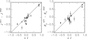
Differences between the IRSF photometry and the NTT photometry (C10) are plotted against the predicted differences from the I-band light curves. BL stars are indicated by open circles and WV stars by filled circles.
3 PERIOD–LUMINOSITY RELATIONS OF TYPE II CEPHEIDS
3.1 PLRs of the SMC T2Cs
Fig. 2 shows the phase-corrected JHKs data plotted against log P for the SMC T2Cs based on our data alone. The BL and WV stars (the filled circles) show well-defined PLRs in all the JHKs bands. In contrast, pWs (squares) and RVs (open circles) show a large scatter and are brighter than the PLRs of the BL and WV stars. These objects are discussed in Section 5.
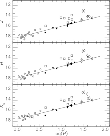
Period–magnitude relations of T2Cs in the SMC. The phase-corrected JHKs magnitudes are plotted against periods. Open circles indicates BL stars and filled circles WV stars. The lines show the PLRs for the combined sample of BLs and WVs. RV and pW stars are indicated by diamond symbols and squares. Error bars are drawn if the photometric errors are larger than 0.05 mag.
PLRs were calculated for BLs and WVs alone and for the combined sample of BL and WV stars. We also derived reddening-free PLRs for the S10 VI data using the indices, Wi (VI) =I−RVIi (V−I), where RVI1 = 1.55 and RVI2 = 1.45 corresponding to two reddening laws as in M09. Table 2 also gives similar relations for the T2Cs in the LMC and those in globular clusters, using the data in M09 and M06. There are not sufficient data to derive PLRs in VI for the globular cluster objects.
Period–luminosity relations of T2Cs. The slope, zero-point near the median period, residual scatter σ and the sample size N are listed for each group. The relations in JHKs bands are derived using only the IRSF data. Those indicated as J† and Ks† are obtained from the combined IRSF and NTT (C10) data sets. The reddening-free indices Wi(VI) are defined in the text. For the LMC/SMC JHKs observations, phase corrections have been applied. Mean magnitudes were obtained from repeated photometry for globular clusters objects. The PLRs for globular clusters are from M06 and those for the LMC from M09.
| Band | Group | Type | Slope | Zero (@log P0) | σ | N |
| J | SMC | BL | −2.545 ± 0.764 | 17.393 ± 0.112 (@0.3) | 0.41 | 15 |
| J | SMC | WV | −2.667 ± 0.246 | 15.483 ± 0.059 (@1.2) | 0.16 | 10 |
| J | SMC | BL+WV | −2.147 ± 0.154 | 15.506 ± 0.116 (@1.2) | 0.34 | 25 |
| H | SMC | BL | −2.765 ± 0.731 | 17.080 ± 0.108 (@0.3) | 0.40 | 15 |
| H | SMC | WV | −2.655 ± 0.236 | 15.129 ± 0.057 (@1.2) | 0.15 | 10 |
| H | SMC | BL+WV | −2.214 ± 0.148 | 15.141 ± 0.112 (@1.2) | 0.32 | 25 |
| Ks | SMC | BL | −2.096 ± 0.732 | 16.933 ± 0.104 (@0.3) | 0.37 | 13 |
| Ks | SMC | WV | −2.844 ± 0.305 | 15.038 ± 0.073 (@1.2) | 0.20 | 10 |
| Ks | SMC | BL+WV | −2.082 ± 0.151 | 15.091 ± 0.109 (@1.2) | 0.32 | 23 |
| J† | SMC | BL | −2.690 ± 0.488 | 17.325 ± 0.069 (@0.3) | 0.36 | 31 |
| J† | SMC | WV | −2.460 ± 0.277 | 15.486 ± 0.073 (@1.2) | 0.24 | 16 |
| J† | SMC | BL+WV | −2.092 ± 0.116 | 15.495 ± 0.092 (@1.2) | 0.33 | 47 |
| Ks† | SMC | BL | −2.553 ± 0.444 | 16.924 ± 0.061 (@0.3) | 0.32 | 29 |
| Ks† | SMC | WV | −2.568 ± 0.247 | 15.041 ± 0.065 (@1.2) | 0.22 | 16 |
| Ks† | SMC | BL+WV | −2.113 ± 0.105 | 15.063 ± 0.082 (@1.2) | 0.29 | 45 |
| W1(VI) | SMC | BL | −2.421 ± 0.479 | 16.832 ± 0.069 (@0.3) | 0.26 | 17 |
| W1(VI) | SMC | WV | −3.003 ± 0.158 | 14.721 ± 0.040 (@1.2) | 0.10 | 10 |
| W1(VI) | SMC | BL+WV | −2.304 ± 0.107 | 14.789 ± 0.083 (@1.2) | 0.23 | 27 |
| W2(VI) | SMC | BL | −2.430 ± 0.488 | 16.894 ± 0.070 (@1.2) | 0.27 | 17 |
| W2(VI) | SMC | WV | −2.985 ± 0.153 | 14.811 ± 0.039 (@0.3) | 0.10 | 10 |
| W2(VI) | SMC | BL+WV | −2.277 ± 0.108 | 14.878 ± 0.085 (@1.2) | 0.24 | 27 |
| J | LMC | BL | −2.164 ± 0.240 | 17.131 ± 0.038 (@0.3) | 0.25 | 55 |
| J | LMC | WV | −2.337 ± 0.114 | 15.165 ± 0.030 (@1.2) | 0.18 | 82 |
| J | LMC | BL+WV | −2.163 ± 0.044 | 15.194 ± 0.029 (@1.2) | 0.21 | 137 |
| H | LMC | BL | −2.259 ± 0.248 | 16.857 ± 0.039 (@0.3) | 0.26 | 54 |
| H | LMC | WV | −2.406 ± 0.100 | 14.756 ± 0.027 (@1.2) | 0.16 | 82 |
| H | LMC | BL+WV | −2.316 ± 0.043 | 14.772 ± 0.028 (@1.2) | 0.20 | 136 |
| Ks | LMC | BL | −1.992 ± 0.278 | 16.733 ± 0.040 (@0.3) | 0.26 | 47 |
| Ks | LMC | WV | −2.503 ± 0.109 | 14.638 ± 0.029 (@1.2) | 0.17 | 82 |
| Ks | LMC | BL+WV | −2.278 ± 0.047 | 14.679 ± 0.029 (@1.2) | 0.21 | 129 |
| W1(VI) | LMC | BL | −2.598 ± 0.094 | 16.597 ± 0.017 (@0.3) | 0.10 | 55 |
| W1(VI) | LMC | WV | −2.564 ± 0.073 | 14.333 ± 0.019 (@1.2) | 0.11 | 76 |
| W1(VI) | LMC | BL+WV | −2.521 ± 0.022 | 14.339 ± 0.015 (@1.2) | 0.11 | 131 |
| W2(VI) | LMC | BL | −2.572 ± 0.093 | 16.665 ± 0.016 (@0.3) | 0.10 | 55 |
| W2(VI) | LMC | WV | −2.551 ± 0.073 | 14.431 ± 0.019 (@1.2) | 0.11 | 76 |
| W2(VI) | LMC | BL+WV | −2.486 ± 0.022 | 14.440 ± 0.015 (@1.2) | 0.11 | 131 |
| J | Globular | BL | −2.959 ± 0.313 | −1.541 ± 0.041 (@0.3) | 0.11 | 7 |
| J | Globular | WV | −2.204 ± 0.090 | −3.543 ± 0.027 (@1.2) | 0.16 | 39 |
| J | Globular | BL+WV | −2.230 ± 0.053 | −3.542 ± 0.024 (@1.2) | 0.16 | 46 |
| H | Globular | BL | −2.335 ± 0.335 | −1.847 ± 0.044 (@0.3) | 0.12 | 7 |
| H | Globular | WV | −2.337 ± 0.086 | −3.942 ± 0.025 (@1.2) | 0.16 | 39 |
| H | Globular | BL+WV | −2.344 ± 0.050 | −3.944 ± 0.023 (@1.2) | 0.15 | 46 |
| Ks | Globular | BL | −2.294 ± 0.294 | −1.864 ± 0.039 (@0.3) | 0.10 | 7 |
| Ks | Globular | WV | −2.442 ± 0.082 | −3.997 ± 0.024 (@1.2) | 0.15 | 39 |
| Ks | Globular | BL+WV | −2.408 ± 0.047 | −4.004 ± 0.021 (@1.2) | 0.14 | 46 |
Dispersions (σ) about the various PLRs are listed in Table 2. For the LMC/SMC samples, these tend to be greater for the BLs than for the WVs. Such differences though suggestive are of only marginal significance. An extreme example is for the log P−W1(VI) in the SMC where σ is 0.26 for the BLs and 0.10 mag for the WVs. However, an F-test shows that this is not significant at the 95 per cent confidence level. In the case of the BL stars in the SMC the C10 data alone show a smaller scatter (0.26 mag) than the IRSF data (0.37 mag) in Ks, which probably indicate a larger observational scatter for the faintest stars in the latter sample. It should be noted that in the case of the LMC we followed Soszyński et al. (2008b) and M09 in omitting a few bright BL stars as possible binaries or blends, while no BL stars were omitted from the SMC sample. Although no evidence of such binarity or blend has been reported for the SMC BL stars, this may well affect the comparison of the σ values.
3.2 Comments on the PLR slopes
Fig. 3 shows PLRs in J and Ks for the SMC based on the combined sample of C10 and the present paper. This consists of 16 measurements of BLs and 31 of WVs (29 at Ks), all of which were corrected for phase variation, for BLs and WVs. C10 derived a distance modulus of 18.85 mag for the SMC by comparing their combined BL+WV sample with the PLRs in J and Ks derived for globular cluster T2Cs by M06. In Fig. 3 these relations are shown as dashed lines for the distance derived by C10. The solid lines are least-squares fit to the data. Apparently the dashed lines with the cluster slopes do not fit the data. This is particularly noticeable in Ks where the best fit with a line of cluster slope is too bright by 0.21 mag at log P = 1.3 and too faint by 0.09 mag at log P = 0.3. This discrepancy, although present, is not as clear from C10 data alone since they had only two long-period WV stars.
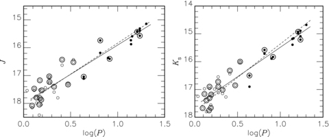
Period–luminosity relations in J and Ks for the combined IRSF and NTT (C10) data set. BL and WV stars are indicated by open and filled circles and those taken from C10 are encircled in addition. The solid lines indicate the least-squares solutions, while the dashed lines show the relations used by C10 to derive an SMC modulus.
The slopes listed in Table 2 show that, in fact, there is a general trend for the PLR slopes to become more negative as one goes from the SMC to the LMC and to the globular clusters. The BL+WV samples have the slopes, in the Ks band, of −2.113 ± 0.125, −2.278 ± 0.047 and −2.408 ± 0.047, and in W1(VI) for the SMC and LMC the slopes are −2.304 ± 0.107 and −2.521 ± 0.022. It should be noted, on the other hand, that the slopes of either the BLs or of the WVs taken by themselves are very uncertain due to the small period range and the relatively small number of stars in each group. The difference in slope between systems may be caused by metallicity and/or age effects although these parameters of the T2Cs are unknown for the Magellanic Clouds. Evidently an SMC distance, and to a lesser extent an LMC distance, based on the cluster data will vary according to the period at which the comparison is made.
4 THE DISTANCE DIFFERENCE BETWEEN THE MAGELLANIC CLOUDS
4.1 Possible effects of Magellanic Cloud structure
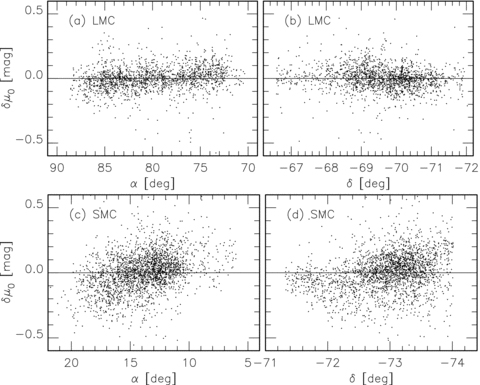
The Magellanic Clouds are close enough to us that their three dimensional structure could affect the relative mean distance of different groups of stars These structures have been studied using several tracers: e.g. classical Cepheids (e.g. Caldwell & Coulson 1986; Groenewegen 2000), red variables Lah, Kiss & Bedding (2005) and red-clump giants (Subramanian & Subramaniam 2009). These authors discussed the internal structures of the Clouds, especially a large line-of-sight depth and substructures of the SMC. Fig. 4 plots the deviations, Δμ0, from the log P–W1(VI) relation against RA and Dec. for both Clouds. We used the PLRs derived for the BLs and WVs separately to estimate their Δμ0 values. These plots are similar to those for classical Cepheids (Fig. A2). In particular the spread is much wider for the SMC than for the LMC due to its large depth. Other major features known from the classical Cepheids are also seen in the T2Cs; e.g. the north-east part of the SMC is closer than the main body. The apparent larger scatter for the BLs compared with the WVs in the SMC may not be significant (see Section 3.1). The zero points of the PLRs correspond to the barycentres of the whole sample, which are indicated by the horizontal lines in Figs 4 and A2. The distances discussed in the following refer to these barycentres.
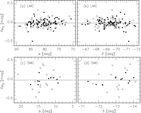
The scatter of the distance moduli of individual T2Cs in the LMC, panels (a) and (b), and in the SMC, (c) and (d) plotted against RA and Dec. BL and WV stars are indicated by open and filled circles. The horizontal lines indicate the barycentres which are determined by the PLRs. A positive δμ0 means that the object is more distant than the centre.
The scatter in the distance moduli of individual classical Cepheids in the LMC, panels (a) and (b), and SMC, (c) and (d). Refer to the caption of Fig. 4.
4.2 The distance difference from the PLRs of Cepheids
In view of the results of Section 3.2 we have derived the difference in moduli of the two Clouds independently for the BLs and WVs. This minimizes any effect on the results of the choice of slopes for PLRs. In this section we also compare these results with those for fundamental mode, classical Cepheids, using the results of Appendix A. For both types of Cepheids, the samples were collected from the same data sets: the OGLE-III variability search in the optical and the IRSF survey in the near-IR.
Table 3 compares the Δμ0 values, in Ks and W(VI), from the classical Cepheids and the T2Cs. The Δμ0 are estimated individually for the groups with different period ranges: three groups with the thresholds of 0.4 and 1.0 in log P for classical Cepheids, and BL (log P < 0.6) and WV (log P > 0.6) for T2Cs. We here consider the Ks-band PLR for the SMC obtained for the combined data sets of C10 and ours, but the results are not affected if only our photometry is used. In the use of the Ks-band PLR, we make corrections for extinctions of EB−V = 0.074 and 0.054 for the LMC and SMC, respectively, (Caldwell & Coulson 1985) according to the extinction law of Cardelli, Clayton & Mathis (1989).
The SMC–LMC modulus difference (Δμ0) derived from the PLRs of T2Cs and classical Cepheids. No corrections for metallicity effects have been applied.
| Type (or log P range) | Δμ0 | ||
| From Ks | From W1(VI) | From W2(VI) | |
| Type II Cepheids | |||
| BL | 0.19 ± 0.07 | 0.24 ± 0.07 | 0.23 ± 0.07 |
| WV | 0.40 ± 0.07 | 0.39 ± 0.05 | 0.38 ± 0.04 |
| BL+WV | 0.38 ± 0.11 | 0.45 ± 0.08 | 0.44 ± 0.08 |
| Classical Cepheids | |||
| 0.0–0.4 | 0.530 ± 0.012 | 0.543 ± 0.009 | 0.537 ± 0.010 |
| 0.4–1.0 | 0.484 ± 0.008 | 0.482 ± 0.008 | 0.476 ± 0.008 |
| 1.0–1.7 | 0.478 ± 0.025 | 0.486 ± 0.025 | 0.479 ± 0.024 |
| 0.4–1.7 | 0.495 ± 0.011 | 0.484 ± 0.010 | 0.480 ± 0.009 |
4.2.1 Δμ0 from classical Cepheids
For the classical Cepheids with log P > 0.4 the results agree well with previous estimates (e.g. Groenewegen 2000). A larger Δμ0 value is indicated at the shorter periods. In the SMC, the PLR slopes at these short periods are different from the longer period ones. This is not the case in the LMC. This suggests that they are less suitable for measuring distance differences at least in the LMC/SMC metallicity range (see also Appendix A).
Metallicity effects on the PLRs of classical Cepheids have been the subject of many publications. On the observational side, two methods are frequently used: (i) comparing Cepheids located in a galaxy at different distances from its centre and thus characterized by different abundances (e.g. Freedman & Madore 1990; Macri et al. 2006; Scowcroft et al. 2009), and (ii) comparing Cepheid-based distances with those obtained with an independent distance indicator, most often the tip of Red Giant Branch (RGB) (e.g. Sakai et al. 2004; Bono et al. 2010). Recently, Bono et al. (2010) investigated the metallicity effects on the PLRs of classical Cepheids from both the observational and theoretical sides and found that these effects were small in W(VI) for a broad range of metallicities. Taking into account estimates in the literature, we consider here a range in the metallicity effect of 0 to −0.3 mag dex−1, for the classical Cepheids with log P > 0.4. The metallicity difference between the Clouds, ∼0.4 dex (Romaniello et al. 2008), leads to the correction of 0–0.1 mag. We adopt a mean value, i.e. 0.05 ± 0.05 mag, which leads to a metallicity corrected value of Δμ0cor = 0.43 ± 0.05 mag. The error is dominated by the uncertainty of the metallicity correction.
4.2.2 Δμ0 from type II Cepheids
No theoretical predications seem to have been made for metallicity effects for T2Cs. However, the results for T2Cs in globular clusters (M06), which are heavily weighted to WV stars, suggest that at Ks any such effects are small. The present results support this conclusion since the Δμ0 values for the WV stars in Table 3 are in satisfactory agreement with the metallicity corrected value for the longer period classical Cepheids.
On the other hand, the Δμ0 value from the BL stars is smaller than for the WVs or classical Cepheids. This is a result at the 2σ level and is present both in Ks and VI. This points to a difference in mean properties of BLs in the LMC and SMC. Mean metallicity or age differences are the most likely candidates.
4.3 Comparison with other methods
Various other estimates of the difference in the distance moduli of the Clouds, Δμ0, are listed in Table 4. This table also shows the results for WV stars, and the longer period classical Cepheids.
The SMC–LMC modulus difference, Δμ0, derived in various ways. The values corrected for metallicity and/or other population effects, Δμ0cor, are also listed. Their errors include the uncertainty of this correction. References are indicated in the last column.
| Method | Δμ0 | Δμ0cor | Notes | Ref. |
| Type II Cepheids (WV) | 0.40 ± 0.07 | – | (1) | This work |
| 0.39 ± 0.05 | – | (2) | This work | |
| Classical Cepheids | 0.48 ± 0.01 | 0.43 ± 0.05 | (1,3,4) | This work |
| 0.48 ± 0.01 | 0.43 ± 0.05 | (2,3,4) | This work | |
| 0.48 ± 0.04 | 0.43 ± 0.06 | (1,3) | Groenewegen (2000) | |
| 0.51 ± 0.02 | 0.46 ± 0.05 | (2,3) | Groenewegen (2000) | |
| 0.41 ± 0.20 | 0.39 ± 0.20 | (1) | Bono et al. (2010) | |
| 0.45 ± 0.12 | 0.44 ± 0.12 | (2) | Bono et al. (2010) | |
| RR Lyrae variables | 0.327 ± 0.002 | 0.363 ± 0.04 | (1,5) | Szewczyk et al. (2009) |
| Red clump giants | 0.47 ± 0.03 | 0.43 | (1,6) | Pietrzyński, Gieren & Udalski (2003) |
| 0.38 ± 0.02 | 0.45 ± 0.10 | (2) | Pietrzyński et al. (2003) | |
| Tip of RGB | – | 0.40 ± 0.12 | (2,7) | Sakai et al. (2004) |
| Pulsating M giants | 0.41 ± 0.02 | – | (1,8) | Tabur et al. (2010) |
| Eclipsing binaries | – | 0.5 ± 0.15 | (9) | – |
Notes. (1) Based on near-IR photometry, Ks or K. (2) Based on optical photometry, I or W(VI). (3) Our adopted metallicity correction, 0–0.1 mag, was used to derive Δμ0cor. (4) Only those with 0.4 < log P < 1.0 were used. (5) Taking the means of the values based on different calibrations discussed in Szewczyk et al. (2009). (6) The population correction suggested by Salaris & Girardi (2002) was used. (7) A metallicity correction was derived using the colour of the RGB. (8) Tabur et al. (2010) concluded that the metallicity effect is negligible. (9) This value is a rough estimate (see text).
Szewczyk et al. (2008, 2009) used near-IR PLRs of RR Lyraes to derive the distance moduli of the Clouds. They adopted mean metallicities for the LMC and SMC RR Lyraes of −1.48 and −1.7 dex. This leads to changes in Δμ0 of 0.02–0.05 mag depending on which metallicity dependent calibration of the PLR is adopted. These corrections bring the difference into better agreement with the WVs and classical Cepheids. Interestingly, the metallicity correction for RR Lyraes has the same sign as that suggested for BLs above.
Hilditch, Howarth & Harries (2005) obtained an SMC distance modulus of 18.91 ± 0.1 mag from eclipsing binaries, while a larger value, 19.11 ± 0.03 mag, was obtained by North et al. (2010). The difference in these values may come partly from the internal structure of the SMC, but other factors seem to be involved. One of these is the use of different surface brightness–colour relations. These tend to be especially uncertain for the early-type binaries which have generally been used. The method is also sensitive to reddening estimates. The available distance estimates for the LMC from early-type binaries show a rather large scatter (see e.g. Nelson et al. 2000). Pietrzyński et al. (2009) derived an LMC distance modulus of 18.50 ± 0.06 based on a binary system composed of two late-type giants. In Table 4, Δμ0=∼0.5 ± 0.15 mag is adopted.
For red clump stars, Pietrzyński et al. (2003) obtained Δμ0 = 0.47 ± 0.03 mag from K magnitudes. A population correction by Salaris & Girardi (2002) leads to 0.43 mag. Tabur et al. (2010) compared the PLR sequences of pulsating M-type giants, i.e. semiregulars and Miras, in the Magellanic Clouds and those in the solar neighbourhood, finding Δμ0 = 0.41 ± 0.02 mag. They concluded that the metallicity effect for their PLRs is negligible.
In summary, the mean uncorrected Δμ0 for the WVs is 0.39 ± 0.05 mag. This agrees well with the other results in Table 4. These, corrected for metallicity and age effects where necessary, range from 0.36 to 0.46 mag (while eclipsing variables giving ∼0.5 mag). Thus any effect due to population differences on the WVs appear to be small. On the other hand, the smaller Δμ0 for the BLs, together with the result shown in Fig. 3, suggests that the population difference between the two Clouds is affecting the mean luminosities of these stars.
5 THE PERIODS AND COLOURS OF TYPE II CEPHEIDS IN DIFFERENT SYSTEMS
5.1 Period distribution of type II Cepheids
Fig. 5 compares the period distributions of the T2Cs in the Magellanic Clouds and in globular clusters. The pW stars are not included in this comparison. The sample for globular clusters has been slightly changed from that in M09 to include the T2Cs in NGC 6388 and 6441 (table 7 in Pritzl et al. 2003).
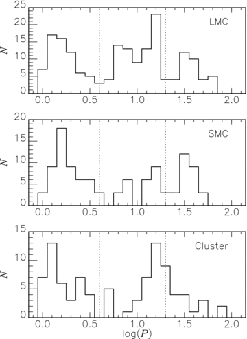
Histograms of periods for the T2Cs in the LMC (top), SMC (middle) and globular clusters (bottom). The pW stars are not included. Vertical lines show the thresholds, 4 and 20 d, used to divide BL, WV and RV variables.
A separation between WV and RV stars is evident for the LMC and SMC samples, while the distribution of the cluster sample suggests that the stars in the RV period range are just the tail of the WV star distribution. This together with the fact that cluster variables in the RV period range lie on an extension of the cluster T2C PLR indicates a fundamental difference from those in the Clouds which lie about PLRs fitted to shorter period T2Cs. There is a suggestion that the relative frequency of variables with log P∼ 0.8 is greater in the LMC than the clusters.
There is a difference in the relative frequencies of WV and BL stars between the LMC and the SMC. The ratio of the two types, NWV/NBL, is 1.25 ± 0.2 for the LMC and 0.6 ± 0.2 for the SMC, where the Poisson noise is considered as the uncertainty. Although the LMC ratio changes if we exclude the conspicuous group of the LMC WV stars with log P∼ 0.8, it would still be larger than the ratio for the SMC. To test for a metallicity effect in this ratio, the globular cluster sample was divided into three groups: 11 objects with [Fe/H] < −1.9, 53 with −1.9 < [Fe/H] < −1.0 and 13 with [Fe/H] > −1 dex. Fig. 6 plots the periods of the globular T2Cs against their metallicities (taken from Harris 1996). We do not include in the discussion the objects in ω Cen, indicated by the cross symbols in Fig. 6, because this cluster has a significant spread in [Fe/H]. Adopting P = 4, 20 d as the dividing lines of the T2C types, NWV/NBL are 0.1 ± 0.1, 1.9 ± 0.6 and 1.0 ± 0.6 for the three groups. The sample in the most metal-rich range is dominated by NGC 6388 and 6441, the two metal-rich clusters with a peculiar population of RR Lyrae stars (Pritzl et al. 2003). Comparing the WV/BL ratios between the other two metallicity ranges suggests that a metal-poor stellar system has a lower WV/BL ratio. This is qualitatively consistent with above results if the SMC T2Cs are lower in metallicity than the LMC ones. Further discussion will be possible when metallicities have been determined for T2Cs in the Magellanic Clouds.
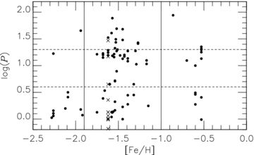
Periods and metallicities of the T2Cs in globular clusters. The cross symbols indicate those in ω Cen plotted at its mean metallicity. The horizontal lines show the divisions between the BL, WV and RV stars, and the vertical lines the adopted divisions by metallicity (see text).
It is interesting that the ratio of long-period to short-period stars is also greater in the LMC than in the SMC for the classical Cepheids (Soszyński et al. 2010a; also see Appendix A). This has generally been attributed to a metallicity effect Becker, Iben & Tuggle (1977). Although not included in Fig. 5, the SMC pW stars have longer periods than their counterparts in the LMC as pointed out in S10 and as can be seen from Fig. A1. The reason for this is not clear. No counterpart to pW stars have been identified in globular clusters.
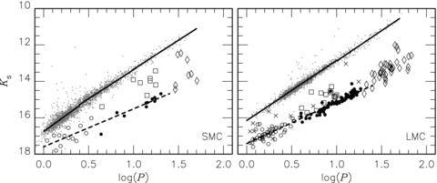
The PLRs at Ks for classical Cepheids in the SMC (left) and LMC (right) (grey dots and filled lines, see Appendix A). Also shown for comparison are the relations for the T2Cs, indicated by dashed lines. Symbols for the T2Cs are the same as in Fig. 2 except the crosses in the LMC sample which indicate stars not used in the least-squares fits (see M09). RVs and pWs are shown as open circles and squares.
5.2 Colours of type II Cepheids
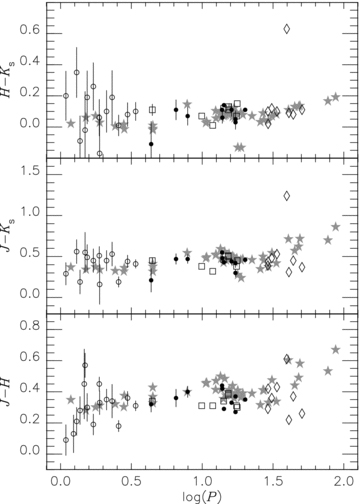
Fig. 7 shows colour–magnitude and colour–colour diagrams for BL, WV, pW and RV variables in the SMC. T2Cs in globular clusters are plotted by grey star symbols in the colour–colour diagrams for comparison. In panel (d), the triangles indicate Galactic RV stars from Lloyd Evans (1985). Their magnitudes were converted from the SAAO system into that of the IRSF using transformations in Carpenter (2001) and Kato et al. (2007). For the cluster variables, the dereddened colours have been adjusted for the mean SMC reddening (EB−V = 0.054 mag, Caldwell & Coulson 1985). The colours of the Galactic RV stars have not been corrected for their reddenings. The curves in the two-colour plots indicate the location of normal giants (G0III–K5III) taken from Bessell & Brett (1988) whose colours are also transformed into the IRSF system after adding the SMC reddening. The distribution of the SMC objects in these plots is similar to that of the LMC objects (fig. 3 in M09).

A colour–magnitude diagram and colour–colour diagrams for T2Cs. Panel (a) includes all types SMC T2Cs, while panels (b), (c) and (d) are for BL, WV/pW and RV stars. Symbols for the SMC T2Cs are the same as in Fig. 2. Grey star symbols indicate the T2Cs in globular clusters (M06). In panel (d), the triangles are for Galactic RV stars from Lloyd Evans (1985). Error bars are drawn for the SMC T2Cs only if an uncertainty exceeds the size of the symbol. The thick curve in the colour–colour diagrams is the locus of local giants from Bessell & Brett (1988).
IR colour/log P relations are plotted in Fig. 8. No correction for interstellar reddening was applied to the SMC objects. The dereddened magnitudes of the globular cluster objects have been reddened by an amount corresponding to the SMC reddening as in Fig. 7, so that the two samples are directly comparable. The WV stars in globular clusters, 1.0 ≤ log P≤ 1.3, have a trend for (J−H) and (J−Ks) to become bluer with increasing period, which is not clear for the SMC WVs. Two pW stars in the SMC, #1 and #11, are separated from the trend of globular WV stars. The lower photometric accuracies for BL stars prevent us from any comparison with the clusters.
Period–colour relations for T2Cs. Symbols are the same as in Fig. 7. Error bars are indicated for the SMC T2Cs only if the uncertainties exceed 0.03 mag.
RV stars show a wider colour distribution and appear to be heterogeneous in nature (see section 5.2 in M09). An SMC RV star, #18, is distinctly red in J−Ks and H−Ks but not in J−H. A few RV stars are similar to the globular objects in H−Ks but bluer in J−H at a given period. These features of the SMC T2Cs are similar to those in the LMC (M09). On the other hand, the two brightest stars, RV stars #7 and #29, are not exceptionally red in any near-IR colour. This is different from the situation in the LMC where the three brightest RV stars have an excess in Ks (M09) as does the SMC RV star #18. In the log P–Ks plot (Fig. A1) #7 and #29 are almost as bright as classical Cepheids with similar periods (see Fig. A1). S10 notes that these two stars are in binary, eclipsing or ellipsoidal, systems.
6 CONCLUSIONS
In this paper PLRs are derived for T2Cs in the SMC. Evidence is presented that T2C PLR slopes differ in three different systems (globular clusters, LMC, SMC) when BL and WV stars are used in combined solutions. Treating the BL and WV stars separately, it was found that the difference in distance moduli between the SMC and LMC derived from WVs alone agrees closely with that obtained from other distance indicators. This implies that the absolute magnitudes of the WVs are, within the uncertainties, free of metallicity effects, which is in agreement with the results derived from globular clusters. On the other hand the SMC–LMC difference is smaller for the BLs and suggests that their absolute magnitudes are not immune from population effects. The relative frequencies of WV to BL stars also varies from system to system.
Phase-corrected data are used throughout this paper although C10 found that this did not reduce the scatter for their sample of stars. None of the conclusions of the paper are significantly affected if uncorrected data are used.
This work is based on the result of the OGLE project. The OGLE has received funding from the European Research Council under the European Community’s Seventh Framework Programme (FP7/2007-2013)/ERC grant agreement no. 246678. We thank the referee (G. Bono) for his useful comments. NM acknowledges the support by the Grant-in-Aid for Research Activity Start-up (No. 22840008) from the Japan Society for the Promotion of Science (JSPS). The work of MWF is supported by South African National Research Foundation.
REFERENCES
Appendix
APPENDIX A: THE PLRS OF CLASSICAL CEPHEIDS
For comparison with the T2Cs, PLRs have been derived for the classical Cepheids in both Clouds found in the OGLE III survey (Soszyński et al. 2008a; Soszyński et al. 2010a). Choosing fundamental mode pulsators only there are 1849 stars in the LMC and 2626 in the SMC. Of these, there are matches within 0.5arcsec, for 1797 and 2436 stars in the IRSF catalogue (Table A1). Among these, 140 and 187 stars were detected in the IRSF survey twice because they are located in overlapping fields of the IRSF survey. These duplicates show that the phase-correction procedure which gives satisfactory results for the T2Cs does not work well for the classical Cepheids. This is probably because of systematically different light curves in I and in JHKs for the latter. We thus use the single-epoch IRSF magnitudes to discuss the near-IR PLRs. This has a negligible effect on the final results because of the large number of stars involved.
The catalogue of OGLE-III classical Cepheids, pulsating in the fundamental mode, with IRSF counterparts. The periods and corresponding IRSF measurements are listed as in Table 1. Shifts for the phase corrections (δφ) obtained from the I-band light curves are also listed, but not used in our plots and fits. This is the first 10 lines of the full catalogue which will be available in the online version of the article (see supporting information). Note that both the LMC and SMC objects are included in a single catalogue, but each OGLE-ID indicates one of the Clouds.
| OGLE-ID | log P | IRSF counterpart | δφ | ||||||||||
| IRSF-Field | MJD(obs) | Phase | J | EJ | H | EH | Ks | EKs | |||||
| OGLE-LMC-CEP-0028 | 0.10139 | LMC0443-6940F | 53036.771 | 0.844 | 16.34 | 0.03 | 16.07 | 0.03 | 15.95 | 0.08 | −0.169 | ||
| OGLE-LMC-CEP-0033 | 0.85617 | LMC0444-6920C | 53036.877 | 0.068 | 13.72 | 0.02 | 13.45 | 0.01 | 13.38 | 0.02 | 0.177 | ||
| OGLE-LMC-CEP-0034 | 1.05133 | LMC0442-7040E | 52693.855 | 0.645 | 13.23 | 0.02 | 12.84 | 0.01 | 12.71 | 0.02 | −0.165 | ||
| OGLE-LMC-CEP-0040 | 0.71308 | LMC0443-6940C | 53034.803 | 0.132 | 13.99 | 0.01 | 13.74 | 0.01 | 13.70 | 0.02 | 0.191 | ||
| OGLE-LMC-CEP-0042 | 0.41112 | LMC0442-7020H | 52692.889 | 0.978 | 14.99 | 0.01 | 14.87 | 0.02 | 14.80 | 0.02 | 0.262 | ||
| OGLE-LMC-CEP-0042 | 0.41112 | LMC0443-7000B | 53039.905 | 0.635 | 15.26 | 0.01 | 14.96 | 0.02 | 14.90 | 0.03 | −0.174 | ||
| OGLE-LMC-CEP-0046 | 0.94663 | LMC0444-6920H | 53498.715 | 0.522 | 13.47 | 0.02 | 13.08 | 0.02 | 12.99 | 0.01 | −0.117 | ||
| OGLE-LMC-CEP-0048 | 0.74418 | LMC0443-6940E | 53034.855 | 0.166 | 13.85 | 0.01 | 13.57 | 0.01 | 13.52 | 0.02 | 0.145 | ||
| OGLE-LMC-CEP-0049 | 0.58536 | LMC0442-7040D | 52692.971 | 0.257 | 14.67 | 0.02 | 14.33 | 0.01 | 14.24 | 0.03 | 0.028 | ||
| OGLE-LMC-CEP-0050 | 0.89463 | LMC0443-6940H | 53037.841 | 0.805 | 13.81 | 0.02 | 13.42 | 0.02 | 13.34 | 0.03 | −0.164 | ||
Fig. A1 shows the Ks-band PLRs of the classical Cepheids in the both Clouds. Those for the T2Cs are also plotted. Classical Cepheids are brighter than T2Cs by 1.0–2.5 mag depending on the periods. The pW/RV stars are located between the PLRs of two types of Cepheids.
The classical Cepheids in each galaxy were divided into three groups according to their periods using divisions at 0.4 and 1.0 in log P. For each group and period range, a least-square fit was obtained with a 3σ clipping applied. (Table A2). Note that no correction of interstellar extinction has been applied [they are of course unnecessary in W(VI)].
Period–luminosity relations for classical Cepheids. Refer to the caption of Table 2.
| Band | Group | Period range | Slope | Zero (@log P0) | σ | N |
| J | LMC | 0.0 < log P < 0.4 | −3.139 ± 0.124 | 15.522 ± 0.012 (@0.3) | 0.16 | 164 |
| J | LMC | 0.4 < log P < 1.0 | −3.138 ± 0.028 | 14.254 ± 0.005 (@0.7) | 0.16 | 1585 |
| J | LMC | 1.0 < log P < 1.7 | −3.053 ± 0.165 | 12.719 ± 0.020 (@1.2) | 0.21 | 119 |
| H | LMC | 0.0 < log P < 0.4 | −3.235 ± 0.099 | 15.231 ± 0.010 (@0.3) | 0.13 | 164 |
| H | LMC | 0.4 < log P < 1.0 | −3.248 ± 0.022 | 13.926 ± 0.004 (@0.7) | 0.12 | 1579 |
| H | LMC | 1.0 < log P < 1.7 | −3.143 ± 0.139 | 12.336 ± 0.017 (@1.2) | 0.18 | 120 |
| Ks | LMC | 0.0 < log P < 0.4 | −3.289 ± 0.099 | 15.160 ± 0.010 (@0.3) | 0.13 | 164 |
| Ks | LMC | 0.4 < log P < 1.0 | −3.284 ± 0.020 | 13.838 ± 0.004 (@0.7) | 0.11 | 1584 |
| Ks | LMC | 1.0 < log P < 1.7 | −3.197 ± 0.135 | 12.231 ± 0.017 (@1.2) | 0.17 | 118 |
| W1(VI) | LMC | 0.0 < log P < 0.4 | −3.325 ± 0.078 | 14.906 ± 0.008 (@0.3) | 0.10 | 160 |
| W1(VI) | LMC | 0.4 < log P < 1.0 | −3.316 ± 0.015 | 13.573 ± 0.003 (@0.7) | 0.08 | 1578 |
| W1(VI) | LMC | 1.0 < log P < 1.7 | −3.189 ± 0.163 | 11.916 ± 0.020 (@1.2) | 0.20 | 121 |
| W2(VI) | LMC | 0.0 < log P < 0.4 | −3.300 ± 0.080 | 14.978 ± 0.008 (@0.3) | 0.10 | 160 |
| W2(VI) | LMC | 0.4 < log P < 1.0 | −3.294 ± 0.015 | 13.654 ± 0.003 (@0.7) | 0.09 | 1579 |
| W2(VI) | LMC | 1.0 < log P < 1.7 | −3.159 ± 0.160 | 12.010 ± 0.019 (@1.2) | 0.20 | 121 |
| J | SMC | 0.0 < log P < 0.4 | −3.381 ± 0.061 | 16.035 ± 0.008 (@0.3) | 0.23 | 1590 |
| J | SMC | 0.4 < log P < 1.0 | −2.992 ± 0.049 | 14.720 ± 0.009 (@0.7) | 0.22 | 862 |
| J | SMC | 1.0 < log P < 1.7 | −3.020 ± 0.128 | 13.171 ± 0.021 (@1.2) | 0.22 | 107 |
| H | SMC | 0.0 < log P < 0.4 | −3.519 ± 0.054 | 15.744 ± 0.007 (@0.3) | 0.20 | 1584 |
| H | SMC | 0.4 < log P < 1.0 | −3.134 ± 0.042 | 14.392 ± 0.007 (@0.7) | 0.19 | 854 |
| H | SMC | 1.0 < log P < 1.7 | −3.110 ± 0.114 | 12.792 ± 0.019 (@1.2) | 0.19 | 107 |
| Ks | SMC | 0.0 < log P < 0.4 | −3.546 ± 0.055 | 15.683 ± 0.007 (@0.3) | 0.20 | 1582 |
| Ks | SMC | 0.4 < log P < 1.0 | −3.176 ± 0.041 | 14.315 ± 0.007 (@0.7) | 0.18 | 854 |
| Ks | SMC | 1.0 < log P < 1.7 | −3.197 ± 0.111 | 12.702 ± 0.018 (@1.2) | 0.19 | 108 |
| W1(VI) | SMC | 0.0 < log P < 0.4 | −3.543 ± 0.043 | 15.449 ± 0.005 (@0.3) | 0.16 | 1596 |
| W1(VI) | SMC | 0.4 < log P < 1.0 | −3.318 ± 0.035 | 14.055 ± 0.006 (@0.7) | 0.15 | 859 |
| W1(VI) | SMC | 1.0 < log P < 1.7 | −3.283 ± 0.093 | 12.402 ± 0.015 (@1.2) | 0.16 | 108 |
| W2(VI) | SMC | 0.0 < log P < 0.4 | −3.521 ± 0.043 | 15.515 ± 0.006 (@0.3) | 0.16 | 1596 |
| W2(VI) | SMC | 0.4 < log P < 1.0 | −3.286 ± 0.035 | 14.130 ± 0.006 (@0.7) | 0.16 | 859 |
| W2(VI) | SMC | 1.0 < log P < 1.7 | −3.250 ± 0.093 | 12.489 ± 0.015 (@1.2) | 0.16 | 108 |
A break in the slope of the PLR at log P∼ 0.4, was first found by Bauer et al. (1999) and confirmed by later work (Soszyński et al. 2010a; and references therein). A break at around log P = 1 has been also claimed especially at optical wavelengths (see e.g. Sandage, Tammann & Reindl 2009). The latter break is less certain than the former and is expected to be less significant, and possibly absent, in the near-IR (see Table 2 in Bono et al. 2010). It is also not present in W(VI) (Bono & Marconi 1999).
The PLRs in the shortest period range, 0.0 < log P < 0.4, are steeper than those at longer periods in the SMC, but not in the LMC. The slope change seems to be a characteristic of Cepheids in a low-metal environment like the SMC and dwarf galaxies (Dolphin et al. 2003). This break has been also confirmed in the Spitzer photometry at the 3.6 and 4.5 μm bands (Ngeow & Kanbur 2010). On the other hand, the slopes for the PLRs at 0.4 < log P < 1.0 and log P > 1.0 are nearly the same and the break at log P∼ 1 is not evident in these data. This is also consistent with previous studies involving the IR PLRs (Ngeow et al. 2009; Marengo et al. 2010; Ngeow & Kanbur 2010).
The residuals of individual classical Cepheids from the PLRs in W1(VI) for each group are plotted in Fig. A2. As in Fig. 4, the distribution for the SMC objects show a larger scatter than that in the LMC and a clear spatial structure. One can also notice a small tilt of the distribution in the LMC, which is barely seen for the T2Cs (Fig. 4). The eastern part of the LMC disc is slightly closer to us than the western part in agreement with previous work (Caldwell & Coulson 1986; Groenewegen 2000).
SUPPORTING INFORMATION
Additional supporting information may be found in the online version of this article:
Table A1. The catalogue of OGLE-III classical Cepheids, pulsating in the fundamental mode, with IRSF counterparts.
Please note: Wiley-Blackwell are not responsible for the content or functionality of any supporting materials supplied by the authors. Any queries (other than missing material) should be directed to the corresponding author for the article.
