Potential–density pairs for bent bars Free

Abstract

1 INTRODUCTION

Bars are a common self-gravitating structure present in disc galaxies. About 50 per cent of such galaxies are strongly or weakly barred, including our Milky Way (Sellwood & Wilkinson 1993; Binney & Merrifield 1998); see also the classification of galaxies by de Vaucouleurs (1963) and the fraction of barred galaxies discussed by Knapen (1999), Eskridge et al. (2000) and Knapen, Shlosman & Peletier (2000). Galactic bars are triaxial systems, and constructing analytical triaxial potential–density pairs is a difficult task. The only exact, self-consistent models of bars were constructed by Freeman (1966), but they have some unrealistic features for barred systems. As alternatives, galactic bars have been approximately modelled as homogeneous ellipsoids (Danby 1965; Michalodimitrakis 1975) or inhomogeneous prolate spheroids (de Vaucouleurs & Freeman 1972; Athanassoula et al. 1983; Papayannopoulos & Petrou 1983; Pfenniger 1984). In these works, the inhomogeneous bar has been represented by a Ferrers (1877) ellipsoid, which has a finite length and represents many features of galactic bars rather well. Long & Murali (1992) found simple analytical potential density–pairs for prolate and triaxial bars that can all be expressed in terms of elementary functions. One of their model of bar was used in hydrodynamic simulations (Lee et al. 1999; Ann & Lee 2000, 2004; Ann & Thakur 2005; Thakur, Ann & Jiang 2009) to understand the response of a gaseous disc to the imposition of non-axisymmetric bar potentials.

Until recently, an unclear issue was the connection between bars and grand-design spirals. Many barred galaxies have spiral arms that appear to emerge from the tips of the bar (see e.g. NGC 1300; Binney & Tremaine 2008, p. 525). However, Sellwood & Sparke (1988) present evidences that the pattern speed of the spirals is much lower than the pattern speed of the bar, so the spiral cannot be driven directly by the bar. On the other hand, there are other observational evidences that bars and spiral arms are correlated (Elmegreen & Elmegreen 1989; Block et al. 2001, 2004; Buta et al. 2009). Salo et al. (2010) recently investigated the relation between bar forcing and spiral density amplitudes for over 100 barred galaxies, and found that there exists a significant statistical correlation. Furthermore, hydrodynamics simulations of the response of a gaseous disc to the imposition of a non-axisymmetric bar (Athanassoula 1992; Wada 1994; Englmaier & Gerhard 1997; Fukuda, Wada & Habe 1998; Ann & Lee 2000; Englmaier & Shlosman 2000; Patsis & Athanassoula 2000; Maciejewski et al. 2002; Maciejewski 2003; Ann & Thakur 2005) have shown that the symmetric two-armed spirals in barred galaxies are driven by the gravitational torques of the bar.

The system bar+spiral arms may be viewed as a bar with bended ends, although we are not aware that such an interpretation has been proposed so far. It would be interesting to have simple, analytical models for such a gravitating system. In this work we propose a method to obtain potential–density pairs for thin and for ‘softened’ bent bars. In Section 2, we present a procedure to bend a thin massive line and to calculate its potential. The idea is to consider a slight curvature and expand the potential with respect to a small parameter. In Section 3 this formalism will be particularized to a thin bar with constant linear density. It will be shown that if the ‘bending function’ can be written in terms of Legendre polynomials, then the potential of the bent bar will be an exact solution of the Laplace equation. Two examples of deformed bars will be discussed. By using a suitable transformation, the thin bent bars are then ‘softened’ to generate three-dimensional potential–density pairs without singularities. In Section 4, we present non-axisymmetric potential–density pairs that represent planar distributions of matter constructed from the two potentials of bent bars discussed in Section 3. These planar potential–density pairs are found by using a method first proposed by Kuzmin (1956). The discussion of the results is left to Section 5.

2 BENT MASSIVE LINES

In this section we present a procedure to bend a thin massive line. The curvature is supposed to be small, and the potential of the bent system will be obtained from an expansion of a small parameter. The undeformed massive line will be described by the parametric equations x′=x₀(t), y′=y₀(t), z′=z₀(t), with t∈[t₁, t₂]. The gravitational potential Φ (r) of this line can be expressed as

1

where G is the gravitational constant, s is the arc length and λ(s) is the linear density. In terms of the parameter t, equation (1) is rewritten as

2

where the dot represents derivative with respect to t.

We shall represent a slight curvature of the line as

3

where r₀(t) is the position of the undeformed line, ɛ is a small dimensionless parameter and the particular form of the curvature will be determined by the function r₁(t). We have, up to first order in ɛ,

4

5

Thus, up to first order in ɛ, the potential (2) can be written as

6

3 BENT BARS

Now we consider the particular case of a bent bar with constant linear density. The undeformed bar located symmetrically on the z-axis with length 2a and linear density λ₀ will be parametrized by r₀ = (0, 0, t), with t∈[−a, a]. For simplicity, the ‘bending function’r₁(t) will be chosen as ⁠. With these assumptions, the potential (6) reduces to

7

where

8

At this point it is convenient to relate the potentials (8) to an identity found by Letelier (1999):

9

where P_n and Q_n are, respectively, the Legendre polynomials and the Legendre functions of the second kind, and (u, v) are the spheroidal coordinates related to the cylindrical coordinates (R, z) through

10

11

with u≥ 1 and −1 ≤v≤ 1. The physical interpretation of (9) is in terms of a bar with linear density proportional to a Legendre polynomial, whose potential corresponds to a multipole term that arises in a multipolar solution of the Einstein equations. The potential Φ₀ in (8) can thus be identified with

12

Furthermore, we note that Φ₁ can be rewritten as

13

If the function f(t) can be expressed as a linear combination of Legendre polynomials, then the last integral in (13) may be directly integrated via the identity (9). This also shows that the potential Φ₁ will be then a solution of the Laplace equation, thus the potential (7) of the bent bar will also be an exact solution of the Laplace equation.

As examples, we will calculate the potential–density pairs for bars with two choices for the ‘bending function’⁠. By (3), the parametric equations of the deformed bar are x′ = 0, y′=ɛf(t) and z′=t, t∈[−a, a], which may be rewritten as y′=ɛf(z′), −a≤z′≤a. We shall take as first example f(t) =t²/a and then f(t) =t³/a². The shape of the bent bar in each case is schematically depicted in Figs 1(a) and (b), respectively. The first shape does not represent necessarily a galactic bar, but we chose this bending function for its simplicity. The second shape mimics a bar with two spiral arms. In terms of Legendre polynomials, we have

14

15

It is then straightforward to calculate the potential (13) using the identity (9), and we state the final result

16

17

where ⁠, and the subscripts (a) and (b) refer to the potentials calculated with the functions f(t) =t²/a and f(t) =t³/a², respectively. The potential (16) remains invariant under the transformations x→−x or z→−z, whereas the potential (17) remains invariant under the transformations x→−x or y→−y, z→−z.

Figure 1

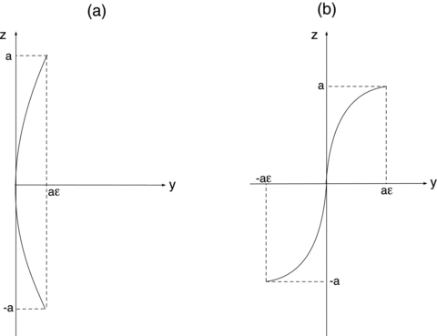
The shape of the bent bar for (a) the function f(t) =t²/a and (b) the function f(t) =t³/a².

Open in new tabDownload slide

3.1 Softened bent bars

The potentials (16)–(17) become singular along the bent thin bars. In order to get physically more realistic potentials it is convenient to ‘soften’ them. A simple way to achieve this is by means of a Plummer-like transformation (Long & Murali 1992). In our examples we apply a transformation x²+y²→x²+y²+b², where b > 0 is a ‘softening’ parameter. The corresponding three-dimensional mass density distribution is obtained from the Poisson equation in Cartesian coordinates, ∇²Φ (x, y, z) = 4πGρ. From the potential (16), after the transformation, we obtain the pair

18

19

where

20

21

where and ⁠. Note that the first term of the potential (18) is the same as the potential of the prolate bar of Long & Murali (1992) with the replacements z→x and x²+y²→y²+z²=R².

Figs 2(a)–(c) display some curves of constant density of the dimensionless mass density ⁠, equation (19), in the three orthogonal planes, with parameters b/a = 0.25 and ɛ = 0.15. The bending of the bar is apparent in the y–z plane in Fig. 2(a). The density contours near the origin are bent in the same manner as the thin line of Fig. 1(a). There are two points of maximum that are shifted to the right of the z-axis, and two points of minimum appear on the opposite side. At these points the mass density may become negative as ɛ is increased; we found that for b/a = 0.25 the density is non-negative for ɛ≲ 0.16. As the parameter b/a is increased for a fixed value of ɛ, the density contours become less elongated, the two points of minimum may disappear, and the two points of maximum move towards the origin. The contours in the x–z plane preserve axial symmetry. 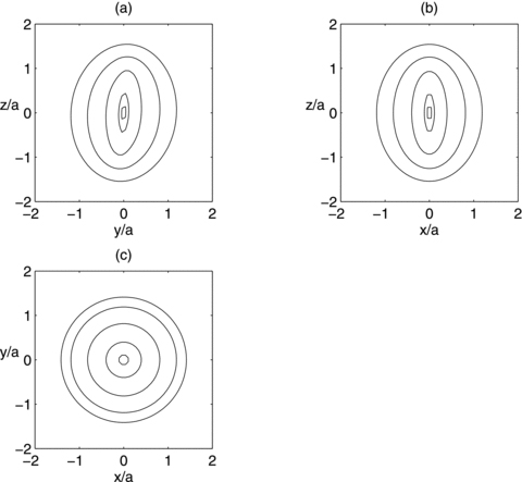Some level curves of the potential ⁠, equation (18), with parameters b/a = 0.25 and ɛ = 0.15, are displayed in Figs 3(a)–(c). In the y–z plane the potential has only one minimum on z = 0 and y=y_m, which is the zero of

22

For the above-mentioned values of parameters the minimum occurs at y_m/a≈ 0.011. The components of the force F_(a)=−∇Φ_(a), corresponding to the potential (18), are listed in Appendix A.

Figure 2

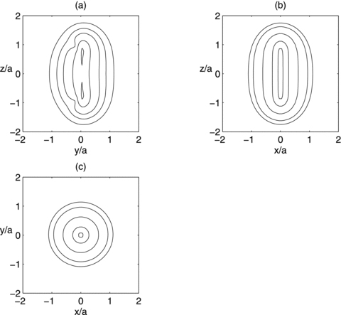
Isodensity contours of the mass density ⁠, equation (19), in the three orthogonal coordinate planes. Parameters: b/a = 0.25 and ɛ = 0.15.

Open in new tabDownload slide

Figure 3

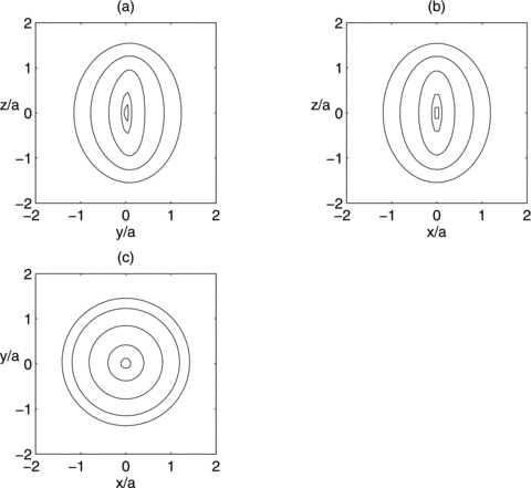
Isopotential contours of the potential ⁠, equation (18), in the three orthogonal coordinate planes. Parameters: b/a = 0.25 and ɛ = 0.15.

Open in new tabDownload slide

Applying the same transformation on the potential (17) results in the potential–density pair:

23

24

where

25

and ρ₀ is given by (20). Some level curves in the three orthogonal planes of the mass density ⁠, equation (24), are shown in Figs 4(a)–(c) with parameters b/a = 0.25 and ɛ = 0.15. The density contours near the origin are bent in the same manner as the thin line of Fig. 1(b). Two points of maximum are present near the z-axis and two points of minimum are located antisymmetrically. The mass density may also become negative at these points with increasing values of ɛ, which can rise up to ɛ≈ 0.18 for b/a = 0.25. When the parameter b/a is increased with fixed ɛ, the point of minimum may disappear, the points of maximum approach the origin and the isodensity contours become more circular, in the same manner as in the previous case. Figs 5(a)–(c) display isopotential curves of the potential ⁠, equation (23), with parameters b/a = 0.25 and ɛ = 0.15. Here the minimum of potential is located at the origin. The components of the force F_(b)=−∇Φ_(b), corresponding to the potential (23), are also given in Appendix A.

Figure 4

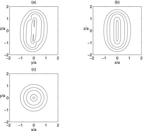
Isodensity contours of the mass density ⁠, equation (24), in the three orthogonal coordinate planes. Parameters: b/a = 0.25 and ɛ = 0.15.

Open in new tabDownload slide

Figure 5

Isopotential contours of the potential ⁠, equation (23), in the three orthogonal coordinate planes. Parameters: b/a = 0.25 and ɛ = 0.15.

Open in new tabDownload slide

4 NON-AXISYMMETRIC THIN DISTRIBUTIONS OF MATTER

Non-axisymmetric thin distributions of matter are of interest since many galaxies exhibit asymmetries in their discs (see e.g. Baldwin, Lynden-Bell & Sancisi 1980; Richter & Sancisi 1994 for observational evidences of asymmetries in disc galaxies). The potential of a thin bent bar may be used to generate non-axisymmetric thin distributions of matter. The procedure is similar to the one proposed by Kuzmin (1956) to find the gravity field of an axisymmetric disc. A source of gravitational field is placed below a plane z = 0. Above the plane this gives a solution of the Laplace equation. The solution valid for z≥ 0 is then reflected with respect to z = 0 so as to give a symmetrical solution of the Laplace equation above and below the plane. This introduces a discontinuity in the normal derivative on z = 0, which by the Poisson equation results in a surface density. Kuzmin applied his procedure on a point mass. In general relativity, where the Schwarzschild solution in Weyl’s metric is represented by a finite bar with constant density, Kuzmin’s method has been used to construct ‘generalized Schwarzschild’ discs (Bičák, Lynden-Bell & Katz 1993a). Some other examples of general relativistic discs generated by Kuzmin’s method can be found in Bičák, Lynden-Bell & Pichon (1993b), Lemos & Letelier (1994), González & Letelier (2000) and Vogt & Letelier (2003).

We will place the thin bent bar along the x-axis and then displace it at a distance c > 0 below the plane z = 0, and make the reflection with respect to that plane. This is equivalent to first make the replacements z→x and x→z in the potentials (16)–(17), and further apply the transformation z→c+ |z|. By Poisson equation, the surface density σ on z = 0 is given by (Binney & Tremaine 2008)

26

For the transformed potentials (16)–(17) we get, respectively,

27

28

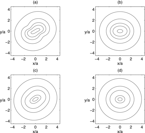
where and ⁠. Note that the first term in (27) and (28) is the surface density of a flat bar given by equation (11) of Long & Murali (1992). Although they obtained the result by convolution of a flat Miyamoto–Nagai disc (which is in fact a Kuzmin disc) with a needle density, our procedure gives the same result. Some contours of the dimensionless surface density are shown in Fig. 6(a), for c/a = 1 and ɛ = 2, and in Fig. 6(b) for c/a = 1 and ɛ = 0. In both figures the level contours are plot for the same set of values. Figs 6(c) and (d) display contours of the potential for the same parameters as in Figs 6(a) and (b), respectively. The isopotentials are also plot for the same set of values in both figures. Comparing the isodensity contours of the flat bent bar in Fig. 6(a) with the flat bar in Fig. 6(b), we note the asymmetry with respect to the x-axis, with two points of minimum located symmetrically with respect to the y-axis. For c/a = 1, the surface density of the flat bent bar is everywhere non-negative provided ɛ≲ 2.2. The isopotential contours of the flat bent bar are shifted along the y-axis, with a point of minimum at x = 0 and y=y_m, which is the zero of

29

an expression similar to (22). For the parameters c/a = 1 and ɛ = 2 we have y_m/a≈ 0.376.

Figure 6

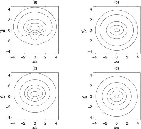
(a)–(b) Isodensity contours of the surface density ⁠, equation (27). (a) Parameters: c/a = 1 and ɛ = 2. (b) Parameters: c/a = 1 and ɛ = 0. (c)–(d) Isopotential contours of the transformed potential for the same parameters as in (a)–(b), respectively.

Open in new tabDownload slide

In Figs 7(a)–(c) we display curves of the surface density along the y- and x-axes for some other values of the parameters c/a and ɛ. In Fig. 7(a) the parameter c/a = 1 is kept constant. With increasing values of ɛ, the asymmetry of the density profile with respect to y = 0 is enhanced. If we maintain ɛ = 2 constant, as in Fig. 7(b), the density distribution becomes somewhat less concentrated as the values of the parameter c/a increase. Fig. 7(c) shows curves of the surface density along the x-axis for the same values of c/a as in Fig. 7(b). From (27), it is seen that for y = 0 the profiles of the surface density of the flat bent bar and of the flat undeformed bar are the same, since the second term in (27) vanishes.

Figure 7

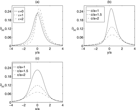
(a)–(b) Profiles of the surface density ⁠, equation (27), along the y-axis, for different values of the parameters. (a) Parameters: c/a = 1 and ɛ = 0, 1 and 2. (b) Parameters: ɛ = 2 and c/a = 1, 1.5 and 2. (c) Profiles of the same surface density along the x-axis. Parameters: c/a = 1, 1.5 and 2.

Open in new tabDownload slide

In Figs 8(a) and (b) we display some contours of the dimensionless surface density ⁠, equation (28), for parameters c/a = 1 and ɛ = 2, and for c/a = 1 and ɛ = 0, respectively. In both figures the level contours are plot for the same set of values. Figs 8(c) and (d) display contours of the potential for the same parameters as in Figs 8(a) and (b), respectively. The isopotentials are also plot for the same set of values in both figures. The surface density as well as the potential for this model of flat bent bar are asymmetric with respect to the x- and y-axes, in contrast to the potential–density pair of the flat undeformed bar. For the parameter c/a = 1, we find that the surface density of this model flat bent bar is everywhere non-negative provided ɛ≲ 3.3. The potential has a point of minimum at the origin. From (28) it is straightforward to see that the surface density profiles along the x- and y-axes are the same for the flat bent and for the flat undeformed bars.

Figure 8

(a)–(b) Isodensity contours of the surface density ⁠, equation (28). (a) Parameters: c/a = 1 and ɛ = 2. (b) Parameters: c/a = 1 and ɛ = 0. (c)–(d) Isopotential contours of the transformed potential for the same parameters as in (a)–(b), respectively.

Open in new tabDownload slide

In Appendix B, we list the components of the force F_(a)=−∇Φ_(a), and of the force F_(b)=−∇Φ_(b) on the plane z = 0, after applying the transformations z→x and x→z, then z→c+ |z|, on the potentials (16)–(17).

5 DISCUSSION

We presented a method to bend a thin massive line when the curvature is small. The potential of the bent system is obtained from an expansion with respect to a small parameter. The procedure was then applied to a homogeneous bar with two examples of ‘bending functions’. We showed that if the ‘bending function’ can be expressed in terms of Legendre polynomials, then the potential of the bent bar is an exact solution of the Laplace equation. Potential–density pairs for ‘softened’ bent bars were constructed by using a Plummer-like transformation. The resulting mass density distributions are non-negative everywhere for restricted values of the deformation parameter ɛ. We also used the potentials of the bent thin bars to construct planar distributions of matter without axial symmetry. Furthermore, non-negative surface density distributions that are non-symmetric with respect to one or both x- and y-axes can be found for restricted values of the deformation parameter ɛ.

We would like to mention that the potential (6) of a bent massive line contains only terms originated from the expansion with respect to ɛ up to first order (dipole terms). In principle, higher order terms can be included, but we found that the explicit expressions, for instance the quadrupole terms, are very cumbersome. In particular, the quadrupolar terms can be explicitly found using the same algorithm employed for the dipolar terms.

A future work will be the study of orbits in the potentials of the ‘softened’ bent bars in an axisymmetric background with and without rotation and comparing the results with the works with undeformed bars (e.g. de Vaucouleurs & Freeman 1972; Athanassoula et al. 1983; Papayannopoulos & Petrou 1983; Pfenniger 1984).

DV thanks FAPESP for financial support. PSL thanks FAPESP and CNPq for partial financial support. Authors also thank the anonymous referee for many comments and suggestions that improved this work. This research has made use of SAO/NASA’s Astrophysics Data System Abstract Service, which is gratefully acknowledged.

REFERENCES

Appendices

APPENDIX A: COMPONENTS OF FORCES FOR BENT BARS

The components of the force F_(a), corresponding to the potential (18), are given by

(A1)

(A2)

(A3)

The components of the force F_(b), corresponding to the potential (23), are given by

(A4)

(A5)

(A6)

In all equations, we have and ⁠.

APPENDIX B: COMPONENTS OF FORCES FOR NON-AXISYMMETRIC THIN DISTRIBUTIONS OF MATTER

The components of the force F_(a)=−∇Φ_(a), on the plane z = 0, after applying the transformations z→x and x→z, then z→c+ |z|, on the potential (16), read

(B1)

(B2)

The components of the force F_(b)=−∇Φ_(b), on the plane z = 0, after applying the transformations z→x and x→z, then z→c+ |z|, on the potential (17), read

(B3)

(B4)

In all equations, we have and ⁠.