


Abstract
Deep narrow-band (NB359) imaging with Subaru telescope by Iwata et al. has detected a surprisingly strong Lyman continuum (LyC; ∼900 Å in the rest frame) from some Lyman α emitters (LAEs) at z= 3.1. However, the possibility of a redshift misidentification by the previous spectroscopic studies due to a narrow wavelength coverage cannot be rejected. Here we present the results of a new technique, the deep spectroscopy, in which we covered 4000–7000 Å with VLT/VIMOS and Subaru/FOCAS for the eight LAEs detected in NB359. All the eight objects have only one detectable emission line around 4970 Å, which is most likely to be Lyα at z= 3.1, and thus, the objects are certainly LAEs at the redshift. However, five of them show a ∼0.8 arcsec spatial offset between the Lyα emission and the source detected in NB359. No indications of the redshifts of the NB359 sources are found although it is statistically difficult that all the five LAEs have a foreground object accounting for the NB359 flux. The rest three LAEs show no significant offset from the NB359 position. Therefore, we conclude that they are truly LyC-emitting LAEs at z= 3.1. We also examine the stellar population which simultaneously accounts for the strength of the LyC and the spectral slope of non-ionizing ultraviolet of the LAEs. We consider the latest statistics of Lyman limit systems to estimate the LyC optical depth in the intergalactic medium (IGM) and an additional contribution of the bound–free LyC from photoionized nebulae to the LyC emissivity. As a result, we find that stellar populations with metallicity Z≥ 1/50 Z⊙ can explain the observed LyC strength only with a very top-heavy initial mass function (IMF; 〈m〉∼ 50 M⊙). However, the critical metallicity for such an IMF is expected to be much lower. A very young (∼1 Myr) and massive (∼100 M⊙) extremely metal-poor (Z≤ 5 × 10⁻⁴ Z⊙) or metal-free (so-called Population III) stellar population can reproduce the observed LyC strength. The required mass fraction of such ‘primordial’ stellar population is ∼1–10 per cent in total stellar mass of the LAEs. We also present a possible evolutionary scenario of galaxies emitting strong LyC and implications of the primordial stars at z∼ 3 for the metal enrichment in the intergalactic medium and for the ionizing background and reionization.
1 INTRODUCTION
The first generation of stars in the Universe is the stellar population without any metal elements, or the so-called Population III (Pop III) stars (e.g. Bromm & Larson 2004). This population is expected to be as massive as ∼100 M⊙ (e.g. Bromm & Larson 2004) and is thought to play an important role on the cosmic reionization at z > 6 (e.g. Loeb & Barkana 2001). How long did such metal-free star formation last in the Universe? Although the metal enrichment in the intergalactic medium (IGM) is uncertain, if it is inefficient, metal-free haloes may form until z = 5 (Trenti, Stiavelli & Shull 2009), z = 2.5 (Tornatore, Ferrara & Schneider 2007) or even z < 2 (Johnson 2010). The metal mixing process in the interstellar medium (ISM) of a galaxy is also uncertain, but a significant amount of metal-free gas may coexist with enriched gas for a few hundred Myr (Pan & Scalo 2007). If it is true, metal-free stars may continue to form in galaxies for such a long time.
The He iiλ1640 emission line is proposed as a signature of Pop III stars because of their very hard ionizing spectrum expected theoretically (Schaerer 2002, 2003). Nagao et al. (2008) made a wide and deep survey of the emission line at z∼ 4 and obtained an upper limit on Pop III star formation rate density at the redshift. On the other hand, the emission line has been found in a composite spectrum of Lyman break galaxies (LBGs) at z∼ 3 (Shapley et al. 2003; Noll et al. 2004). Jimenez & Haiman (2006) claimed that it was a signature of the metal-free stellar population in the LBGs. However, this He ii line is broad (FWHM ∼ 1500 km s−1), and thus, it is probably caused by stellar winds from Wolf–Rayet stars with ‘normal’ metallicity (Shapley et al. 2003; Noll et al. 2004; Brinchmann, Pettini & Charlot 2008).
Another signature of Pop III stars is a very large Lyα equivalent width (EW) as >240 Å (Malhotra & Rhoads 2002). Some surveys of Lyman α emitters (LAEs) found galaxies with such a large Lyα EW at z = 3.1 (Nakamura 2010), z = 4.5 (Malhotra & Rhoads 2002) and z = 5.7 (Shimasaku et al. 2006). However, a clumpy dusty medium may boost the EW only apparently (Neufeld 1991). In addition, there is a large uncertainty on the EW measurements because LAEs are so faint that we may not measure their continuum level accurately enough.
The stellar population with a metal mass fraction (or metallicity) Z < 10−5, which is < 1/2000 Z⊙, is classified as extremely metal-poor (EMP) stars (e.g. Beers & Christlieb 2005) and may be the second generation of stars (Umeda & Nomoto 2003). Hundreds of low-mass EMP stars have been found in the halo of the Galaxy (e.g. Beers & Christlieb 2005). Because of their long lifetime, these stars are survivors of the early stage of the formation of the Galaxy. On the other hand, it is expected that their high-mass counterpart existed in the early days and died out until the current epoch (Tumlinson 2006; Komiya et al. 2007). Yet, there is no direct observational evidence of such massive EMP stars at high z.
Although there is no confident observational signature of primordial massive stellar populations such as Pop III and massive EMP stars so far, these populations should exist in the early universe. These stars emit strong ionizing radiation which should have played an important role in the cosmic reionization (e.g. Loeb & Barkana 2001) and have affected the galaxy formation in the subsequent epoch (e.g. Susa & Umemura 2004). Therefore, looking for these stellar populations is highly important to understand the feedback process by the first generation of stars and galaxies as well as to prove their existence.
Very recently, some candidates of galaxies at z≳ 7 have been discovered by the standard drop-out technique from the new data taken with the WFC3/IR camera on the Hubble Space Telescope (Bunker et al. 2009; Bouwens et al. 2010a; McLure et al. 2010; Oesch et al. 2010; Yan et al. 2010). Interestingly, Bouwens et al. (2010b) found that the ultraviolet (UV) colour of the z≳ 7 candidate galaxies was so blue that the galaxies may be said to be composed of EMP or metal-free stellar populations. However, we should confirm that the redshifts of the galaxies are really z≳ 7 with spectroscopy (Lehnert et al. 2010).
Inoue (2010) (hereafter Paper I) has proposed a new method to find the hypothetical stellar populations like massive EMP and metal-free stars at z≲ 4. When Lyman continuum (LyC) emitted by stars escapes from galaxies, the LyC emitted by photoionized nebulae around ionizing stars may also escape. This bound–free nebular LyC has a peak just below the Lyman limit, so that a spectral ‘bump’ appears at the Lyman limit. We call it ‘Lyman bump’ or more precisely ‘Lyman limit bump’. The strength of the Lyman bump depends on the hardness of the stellar LyC. Thus, more metal poor galaxies will show stronger Lyman bump. On the other hand, neutral hydrogen remains in the IGM even after the completion of the reionization and it significantly absorbs the LyC. This makes it difficult to find LyC or Lyman bump at z > 5 (Inoue & Iwata 2008).
Are there galaxies with a Lyman bump in the real Universe? This paper intends to show that the answer is yes. Iwata et al. (2009) (hereafter I09) discovered 10 LAEs and seven LBGs at z∼ 3 with a significant leakage of their LyC captured in a deep narrow-band image taken with the Subaru/Suprime-Cam (S-Cam). Some of the LAEs are indeed brighter in LyC than in non-ionizing UV, strongly suggesting the presence of the Lyman limit bump. However, there is a possibility that these objects are at a lower z because of a narrow wavelength coverage of the previous spectroscopy which only confirmed an emission line.
The rest of this paper is organized as follows. In Section 2, we first describe the sample of the possible LyC-emitting LAEs discovered by Iwata et al. and reported in I09. In Section 3, we present results of the follow-up spectroscopy with VLT/VIMOS and Subaru/FOCAS. In Section 4, we thoroughly examine the redshift of the LAEs (i.e. the reality of the detected LyC) with the follow-up deep spectra and conclude that at least three LAEs are real LyC emitters. In Section 5, we compare the observed strength of the LyC with the Lyman bump model proposed in Paper I and show that the LAEs are likely to contain massive metal-free or EMP stars. In Section 6, we present a summary of our results, an evolutionary scenario of the LAEs and a few implications of the existence of primordial stars at z∼ 3.
We adopt the AB magnitude system (Oke 1974) to describe object magnitudes and colours in Section 5. The standard flat ΛCDM cosmology with h = 0.7, ΩM = 0.3 and ΩΛ = 0.7 is adopted if it is required.
2 THE SAMPLE OF LAEs EMITTING STRONG LYMAN CONTINUUM
We mainly deal with the sample of LAEs detected in their LyC by I09. Since the detected LyC is too strong to be explained with a standard stellar population model, I09 reported the detections but left their nature as a mystery.
We started from a sample of LAEs and Lyα blobs (LABs) selected through a Subaru/S-Cam narrow-band NB497 imaging in the SSA22 field (Hayashino et al. 2004; Matsuda et al. 2004, hereafter M04). The selection criteria of the LAEs were NB 497 = 20.0–26.2AB (2.0 arcsec ϕ, >5σ) and the observed EW of the emission line >80 Å. Among them, we had 125 galaxies with spectroscopic redshift zspec > 3.0 measured with Subaru/FOCAS and Keck/DEIMOS (Matsuda et al. 2005, 2006; Yamada et al., in preparation). I09 performed a very deep imaging with another narrow-band filter NB359 with Subaru/S-Cam (programme ID: S07B-010) in the same field. The NB359 filter exactly captures LyC (≃880 Å) for z = 3.1 galaxies. In the NB359 image, I09 found 10 objects identified with the spectroscopically confirmed LAEs. The identification of NB359 (and R) sources with the spectroscopic LAEs was done by the following procedure: (1) object detections in NB359 and in R; (2) identification of each LAE with the R object nearest from the barycentre of NB497 intensity; and (3) either identification of an NB359 object within 1.4 arcsec from the barycentre of R intensity or >3σ detection at NB359 aperture photometry with 1.4 arcsec diameter around the barycentre of R intensity. Here we present results of follow-up deep spectroscopy with VLT/VIMOS and Subaru/FOCAS for five out of the 10 LAEs in I09: the objects a–e in Table 1.
Coordinates of the sample galaxies.
| Object | NB359 position | Offset of R | Offset of NB497 | NB359 a | Ra | Spectroscopy | Remarks | ||||
| α (J2000) | δ (J2000) | Δ (arcsec) | PA (°) | Δ (arcsec) | PA (°) | (AB) | (AB) | Previous | Current | ||
| a | 22:17:24.76 | +00:17:16.7 | 0.23 | 22 | 0.38 | 42 | 25.84 | 25.51 | FOCAS in 2005 | VIMOS/FOCAS | I09, LAB35 in M04 |
| b | 22:17:38.97 | +00:17:25.0 | 0.26 | 79 | 0.85 | 43 | 26.28 | 26.66 | FOCAS in 2005 | VIMOS/FOCAS | I09 |
| c | 22:17:45.87 | +00:23:19.1 | 0.24 | 272 | 0.46 | 190 | 26.25 | 26.72 | FOCAS in 2005 | VIMOS | I09 |
| d | 22:17:26.18 | +00:13:18.4 | 0.21 | 297 | 0.88 | 7 | 26.68 | 26.91 | DEIMOS in 2004 | VIMOS | I09 |
| e | 22:17:16.64 | +00:23:07.4 | 0.26 | 76 | 1.06 | 32 | 26.73 | 26.24 | FOCAS in 2005 | VIMOS | I09 |
| f | 22:17:08.04 | +00:19:31.7 | 0.25 | 341 | 0.34 | 7 | 26.88 | 26.52 | – | VIMOS | |
| g | 22:17:53.22 | +00:12:37.4 | 0.00 | – | 0.20 | 257 | 26.84 | 26.84 | FOCAS in 2005 | VIMOS | |
| h | 22:17:29.41 | +00:06:29.0 | 0.41 | 144 | 0.81 | 189 | 26.33 | 26.02 | – | VIMOS | |
| i | 22:17:12.74 | +00:28:55.4 | 0.16 | 4 | 0.12 | 320 | 26.26 | 24.59 | – | VIMOS | broad-line AGN |
aMagnitudes within a 1.2 arcsec diameter aperture at NB359 or R position.
In addition, there are other ∼30 objects detected in the NB359 image and identified with the LAE candidates (i.e. not confirmed spectroscopically yet) by the same procedure described above. Among them, we also present results of deep spectroscopy with VIMOS for four objects: f–i in Table 1.1
In Table 1, we summarize some properties of the sample LAEs: coordinates in NB359 (LyC), offsets and position angles (PAs) of R and NB497 (Lyα) positions against the positions in NB359, and magnitudes in NB359 and R. As found from the table, there are small offsets in the three bands; the offsets between R and NB359 are less than 0.4 arcsec and those between NB359 and NB497 are 0.1–1.0 arcsec. The offsets of the continuum emission traced by R and NB359 of the LAE sample are small and not significant relative to the positional uncertainty between the two bands (∼0.25 arcsec; I09). It is notable that the R–NB359 offsets of the LBG sample reported in I09 are much larger and significant (∼0.97 arcsec on average). On the other hand, in some cases, the offsets between NB359 and NB497 of the LAE sample are significant. This point will be discussed in detail in Sections 3.2 and 4.2.
3 SPECTROSCOPY OF THE LAEs
3.1 Previous medium-resolution spectroscopy
We have several sets of previous spectroscopy with Subaru/FOCAS and Keck/DEIMOS taken in 2003, 2004 and 2005 (Matsuda et al. 2005, 2006; Yamada et al., in preparation) and have confirmed that all the 10 LAEs reported by I09 have a prominent emission line at around 4970 Å which was identified as Lyα at z≃ 3.1. DEIMOS observations in 2004 and FOCAS observations in 2005 (Matsuda et al. 2005, 2006, in preparation; Yamada et al., in preparation) were made with a relatively high spectral resolution (R∼ 2000) and they rejected the possibility that the emission line is the [O ii]λ3727 doublet at z = 0.33. However, the FOCAS observations in 2005 could not exclude the possibility that the line was C ivλ1549, He iiλ1640, C iii]λ1909 or Mg iiλ2798 from an active galactic nucleus (AGN) at redshift z = 2.2, 2.0, 1.6 or 0.78, respectively, or Hβ from a very faint galaxy at z = 0.022 because of a narrow wavelength coverage (Δλ∼ 200 Å). Since the full width at half-maximum (FWHM) of the line was as narrow as 200–600 km s−1, the objects would be type 2 if they were AGNs. However, some of the objects are spatially extended in the NB497 −BV image (i.e. line image), making the AGN interpretation unlikely. For example, the object a is identified as LAB by M04 and the object c has an FWHM of the line intensity profile of 1.3 arcsec against a 1.0-arcsec point spread function (a significance of 3σ).
3.2 VLT/VIMOS low-resolution spectroscopy
We performed a wide wavelength coverage (but low resolution) follow-up spectroscopy for five (objects a–e) out of the 10 LAEs reported in I09 with VLT/VIMOS (programme ID: 081.A-0081). In addition, we took spectra of four (object f–i) LAE candidates detected in the NB359 image. Unlike the previous spectroscopy, we put slitlets on the positions detected in the NB359 image in order to take spectra of NB359-emitting sources.
The observations were made with LR-Blue/OS-Blue grism (R=λ/Δλ≃ 180 and dispersion 5.36 Å pix−1) and 1.0-arcsec width slitlets on several dark nights during July to October 2008. The wavelength coverage of this setting is 3700–6800 Å. The plate scale is 0.205 arcsec pix−1. We took two masks (each has four quadrants) and the exposure time was 4 h for each mask. There was an overlap area of the two masks, so that the object a was taken twice. The observing conditions were good with typical seeing of 0.8 arcsec. The data reduction was done by a standard procedure with iraf. The flux calibration was done with standard stars EG 274, G 158-100 and LTT 1020. The typical sky rms per pixel at around 5000 Å in the resultant two-dimensional spectra is about 0.02 μJy.
Fig. 1 shows close-up images around 5000 Å of the final two-dimensional spectra of the nine objects observed with VLT/VIMOS. In each panel, the area between the two dashed lines indicates 5 pixels (=1.0 arcsec) centring around the position of the NB359 source. To find the NB359 source position, we used an iraf task, geomatch, between the S-Cam image and the VIMOS pre-image. A typical uncertainty of this procedure is found to be ∼0.3 pix (=0.06 arcsec). We also found a few pix systematic offset between the pre-image and the spectral images and corrected it based on the position of some bright objects detected in both images (not the LAEs discussed in this paper).
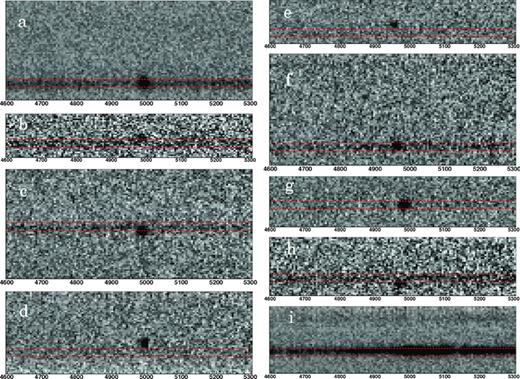
Close-up around 5000 Å of the final two-dimensional spectra taken with VLT/VIMOS. The dotted lines in each panel show 5 pixels (1.0 arcsec) centring around the NB359 source position along the slitlet. North is up.
As found in Fig. 1, a significant spatial offset between the emission line and the NB359 position is evident in some objects. The measured spatial offsets are summarized in Table 2 and consistent with those in Table 1 measured in the two narrow-band images. Relatively large offset in the narrow-band images of the object a is probably due to the extended Lyα emission classified as LAB. We categorize objects a, f and g into the sample without line offset (i.e. offset <0.2 = 1 arcsec pix−1) and objects b–e and h into the sample with line offset based on the spectral image. The reason why we rely on the spectral image is that we can measure the offset between the continuum position and the pure emission line, whereas the NB497 intensity traces both the line and the continuum. The last object i is found to be a broad-line AGN from the spectrum.
A summary of the VLT/VIMOS spectroscopy.
| Object | Line offset (arcsec)a | zLyα | Decrementb |
| Without line offset | |||
| a (con/emi) | 0.12 | 3.100 | 0.90 ± 0.04 |
| f (con/emi) | 0.06 | 3.075 | 0.77 ± 0.11 |
| g (con/emi) | 0.10 | 3.094 | 0.70 ± 0.16 |
| Compositec | – | – | 0.80 ± 0.07 |
| With line offset | |||
| b (con) | 0.62 | – | 1.18 ± 0.29 |
| (emi) | – | 3.090 | 0.54 ± 0.29 |
| c (con) | 0.51 | – | 0.94 ± 0.15 |
| (emi) | – | 3.095 | 1.38 ± 0.31 |
| d (con) | 1.29 | – | 1.49 ± 0.68 |
| (emi) | – | 3.100 | 0.77 ± 0.35 |
| e (con) | 1.00 | – | 1.31 ± 0.44 |
| (emi) | – | 3.065 | 0.69 ± 0.24 |
| h (con) | 0.76 | – | 0.73 ± 0.11 |
| (emi) | – | 3.080 | 0.87 ± 0.23 |
| Compositec (con) | – | – | 1.12 ± 0.15 |
| Compositec (emi) | – | – | 0.86 ± 0.13 |
| AGN | |||
| i (con/emi) | 0.25 | 3.11d | 0.72 ± 0.03 |
aSpatial offsets between the position detected in NB359 and the emission line.
bFlux density ratios between 1050–1150 and 1250–1350 Å in the rest frame of the Lyα redshift. Uncertainties are estimated from the quadratic combination of mean error of the continuum level and sky rms noise. The Galactic dust extinction has been corrected.
cAverage composite based on zLyα.
dThis redshift was determined from metal lines.
Figs 2 and 3 show the one-dimensional spectra extracted at the NB359 source positions of the samples without and with the line offset, respectively. Fig. 4 shows the spectrum of the object i which is identified as a broad-line AGN. In Table 2, we also list the redshifts measured assuming the emission line to be Lyα and the flux density decrements of the continua blueward and redward from the line. We measured the decrements both at the NB359 source position and at the emission line position for the sample with line offset. We have corrected the decrements for the dust extinction by the Galaxy based on the extinction map by Schlegel, Finkbeiner & Davis (1998). Fig. 5 shows average composite spectra of both samples.
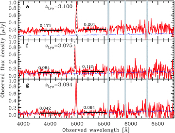
VLT/VIMOS one-dimensional spectra of three objects without offset between the NB359 position and the emission line. The dotted curves are 1σ sky noise spectra. The vertical dashed lines indicate the wavelengths of the emission lines detected in two-dimensional spectra shown in Fig. 1. In each panel, we note the redshift if the emission line is Lyα. The two thick horizontal lines with numbers in each panel show average continuum levels within 1050–1150 Å and 1250–1350 Å in the rest frame for the Lyα redshift. The values are not corrected for the Galactic extinction. The vertical shaded regions show the ranges affected by Earth's atmospheric lines.
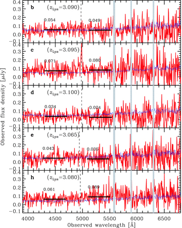
Same as Fig. 2 but for five objects with offset between the NB359 position and the emission line. The spectra are extracted at the NB359 positions.
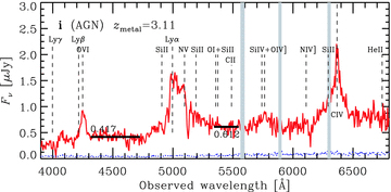
Same as Fig. 2 but for the object identified as a broad-line AGN. The redshift was determined by metal lines indicated by vertical dashed lines. The average continuum level of the longer wavelength is measured within 1300–1350 Å to avoid an effect of the broad Lyα line.
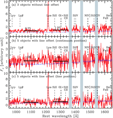
Average composite spectra of (a) three objects without offset between the NB359 position and the emission line (objects a, f and g); (b) five objects with offset (objects b, c, d, e and h); and (c) the same five objects but at the emission line position. The dotted curves are 1σ uncertainty estimated from sky noise spectra. We averaged the one-dimensional spectra in the rest frame for the redshift assuming the emission line to be Lyα. The thick horizontal lines with numbers indicate mean flux densities within 1050–1150 Å and 1250–1350 Å. In the latter wavelength range, we normalized the spectra before making an average. The values are not corrected for the Galactic extinction. The vertical dashed lines indicate wavelengths of emission/absorption lines. The vertical shaded regions show the ranges affected by Earth's atmospheric lines.
3.3 Subaru/FOCAS low-resolution spectroscopy
We have spectra of two objects a and b taken with Subaru/FOCAS (programme ID: S08B-046). The observation was made with the 300B grism (dispersion: 1.34 Å pix−1) and a slitwidth of 0.8 arcsec during the dark night on 2008 September 22. The wavelength coverage of this observation is 4000–7200 Å. The resultant spectrum of the object a is very consistent with those in Fig. 2 but has a higher spectral resolution. On the other hand, we could not find any emission line in the spectrum of the object b. This is because the position angle of the FOCAS slitlet (117°) was far from that of the emission line from the NB359 position (43°; see Table 1). The position angle of the VIMOS slitlet was 0° (north–south) and we did capture a part of the emission line as shown in Fig. 1.
4 REALITY OF THE LYMAN CONTINUUM
In this section, we discuss whether NB359 fluxes detected from the sample LAEs are truly LyC or not. Namely, we discuss whether the redshifts of the continuum sources are z≃ 3.1 or not. As found in Fig. 1, some objects show a spatial offset of the emission line at around 4970 Å. We deal with the two samples with or without the line offset separately.
4.1 Sample without line offset
4.1.1 Line identification
From the objects a, f and g, we clearly detect an emission line at around 4970 Å but obtain no significant spatial offset from the position detected in NB359. Therefore, the emission line is highly likely to come from the continuum source detected in NB359 (see Section 4.1.2 about the probability of foreground contamination). Finally, we conclude that the emission line is Lyα at z≃ 3.1 and the NB359 flux is truly LyC, based on the following considerations.
We could not detect any significant emission/absorption lines except for the 4970-Å line from the three galaxies shown in Fig. 2. The upper limits (3σ) on the line flux ratio relative to the 4970-Å line are <0.10–0.18 at 4000 Å, <0.10–0.18 at 4500 Å, <0.11–0.20 at 5000 Å, <0.15–0.24 at 5500 Å, <0.20–0.35 at 6000 Å and <0.24–0.42 at 6500 Å. These limits are estimated from a comparison between a typical sky rms noise for 5 pix in the spatial direction at a wavelength and the 4970-Å line flux. We assumed that the postulated emission line has the same width as the 4970-Å line. This assumption is justified if the lines are narrower than about 1600 km s−1 (i.e. R≃ 180). These 3σ upper limits of the line flux ratio indicate that we can exclude the existence of other emission lines even if the lines are a factor of 0.1–0.5 weaker than the 4970-Å emission line.
Let us identify the 4970-Å line. We consider seven possible identifications of the line. If the 4970-Å line was C iv and the galaxies were AGNs at z≃ 2.2, we should have the Lyα around 3900 Å. Based on the QSO average spectrum by Francis et al. (1991), the flux ratio of Lyα to C iv is 1.6. Thus, we should be able to detect the Lyα in our spectra with a high significance. However, we could not. We could not detect He ii and C iii] which have flux ratios relative to C iv of 0.3 and 0.5, respectively (Francis et al. 1991; Heckman et al. 1995; Krolik 1999), either. If the 4970-Å line was He ii or C iii] and the galaxies were AGNs at z≃ 2.0 or 1.6, we could detect C iv which is stronger than the two lines (Francis et al. 1991; Heckman et al. 1995; Krolik 1999) at around 4690 or 4030 Å. In the Mg ii case, we could detect a stronger [O ii] emission line from narrow-line regions at around 6630 Å (Krolik 1999). In the [O ii] or the Hβ cases, we could detect stronger [O iii] emission lines at around 6595/6659 Å or 5070/5120 Å, respectively. However, we could not detect these at all. The [O ii] interpretation had already been ruled out by the previous medium-resolution spectra for the objects a–e and g. In the case of Lyα from star-forming galaxies at z = 3.1, we do not expect any other stronger emission lines within the wavelength coverage. Therefore, the single emission line in the wide wavelength coverage strongly suggests that the line is Lyα and the objects lie at z≃ 3.1.
If the galaxies are at z = 3.1, we expect Lyα decrement to be 0.75 ± 0.03 on average at around 1100 Å in rest frame of the galaxies (Inoue & Iwata 2008; Faucher-Giguère et al. 2008) (Note that we are looking at Lyα forest at z = 2.7 in this wavelength.). Let us examine the decrement in the spectra of the three objects (a, f and g) and the AGN (object i). Comparing the flux density within the rest frame 1050–1150 Å to that within 1250–1350 Å with the assumptions of the 4970-Å line to be Lyα and a flat intrinsic spectrum between 1100 and 1300 Å in the rest frame, we find decrements of 0.7–0.9 after correcting for the Galactic extinction as summarized in Table 2. Although the decrement of the object a is somewhat smaller than expected, the other three decrements are very consistent with the Lyα forest measurement, again supporting our interpretation that they are z≃ 3.1 objects.
In summary, the three objects without line offset have a strong and narrow emission line around 4970 Å but do not have any other detectable emission/absorption lines. Their continuum shows a small break below the emission line and the amount of the decrement is consistent with that expected from Lyα forest if they are at z≃ 3.1. Therefore, we conclude that the emission line is redshifted Lyα and the objects are truly LAEs at z≃ 3.1.
4.1.2 Probability of foreground contamination
Even when the emission line around 4970 Å is the z≃ 3.1 Lyα, the LAEs may have a foreground object on the line of sight towards them and the flux detected in NB359 may come from the low-z interloper. This possibility is discussed extensively in Vanzella et al. (2010a) (see also Siana et al. 2007, and I09). Let us estimate the probability to have a contamination in front of the three LAEs discussed in this subsection according to Vanzella et al. (2010a).
The three LAEs without line offset (a, f and g) are detected in NB359 with a magnitude of 26–27 AB (see Table 1) and the spatial offset between the Lyα emission line and the continuum is less than 0.2 arcsec (=1 pix) (see Table 2). Based on the U-band number count by Nonino et al. (2009) of 130 200 deg−2 in this magnitude range, we expect only 0.126 per cent of chance coincidence of an object within 0.2 arcsec around another object.
The object a is found from the 10 objects reported by I09 among 125 spectroscopic LAE sample. The 10 objects may include foreground contamination, but the probability that one object picked up from the 10 objects has a foreground within 0.2 arcsec is only 1.6 per cent.2 The objects f and g are found from ∼30 objects detected in NB359 among ∼800 LAE candidates. If we take two objects from the ∼30 sample, the probability that both of them have a foreground within 0.2 arcsec is only 0.1 per cent and the probability that one of them has a foreground is still 6.5 per cent. Therefore, the three objects a, f and g are unlikely to be contaminated by foreground objects.
4.1.3 Spectroscopic properties
We here note a few more measurements from the spectra. Table 3 is a summary of the derived properties. The FWHMs of Lyα are smaller than the velocity resolution of our observations (≃1600 km s−1). Thus, the linewidth is unresolved. The EWs of Lyα in the rest frame are 20–80 Å in individual spectra and 43 Å in the average spectrum, which are not very large as expected for Pop III stars (e.g. Malhotra & Rhoads 2002; Schaerer 2002). If LyC escape fraction is relatively large, however, the expected EW of Lyα decreases. The EW is further reduced by neutral hydrogen in the ISM and in the IGM because of resonant scattering. Therefore, the measured Lyα EWs do not reject the existence of Pop III stars in the three LAEs.
Spectroscopic properties of the LAEs without line offset.
| Object | zLyα | FWHMa (km s−1) | EW0b (Å) |  |
| a | 3.100 | 1190 | 20.4 ± 1.1 | <0.24 |
| f | 3.075 | 1070 | 29.3 ± 3.4 | <0.40 |
| g | 3.094 | 1130 | 78.5 ± 12.3 | <0.25 |
| Composited | – | 1140 | 43.2 ± 2.9 | <0.21 |
| Object | zLyα | FWHMa (km s−1) | EW0b (Å) | |
| a | 3.100 | 1190 | 20.4 ± 1.1 | <0.24 |
| f | 3.075 | 1070 | 29.3 ± 3.4 | <0.40 |
| g | 3.094 | 1130 | 78.5 ± 12.3 | <0.25 |
| Composited | – | 1140 | 43.2 ± 2.9 | <0.21 |
aFull width at half-maximum of Lyα.
bRest-frame equivalent widths of Lyα. Uncertainties include only statistical errors in estimating the line flux based on sky rms noise.
c3σ upper limits on the He ii line flux relative to Lyα estimated from sky rms noise. The linewidth is assumed to be the same as that of Lyα.
dAverage composite.
Spectroscopic properties of the LAEs without line offset.
| Object | zLyα | FWHMa (km s−1) | EW0b (Å) | |
| a | 3.100 | 1190 | 20.4 ± 1.1 | <0.24 |
| f | 3.075 | 1070 | 29.3 ± 3.4 | <0.40 |
| g | 3.094 | 1130 | 78.5 ± 12.3 | <0.25 |
| Composited | – | 1140 | 43.2 ± 2.9 | <0.21 |
| Object | zLyα | FWHMa (km s−1) | EW0b (Å) | |
| a | 3.100 | 1190 | 20.4 ± 1.1 | <0.24 |
| f | 3.075 | 1070 | 29.3 ± 3.4 | <0.40 |
| g | 3.094 | 1130 | 78.5 ± 12.3 | <0.25 |
| Composited | – | 1140 | 43.2 ± 2.9 | <0.21 |
aFull width at half-maximum of Lyα.
bRest-frame equivalent widths of Lyα. Uncertainties include only statistical errors in estimating the line flux based on sky rms noise.
c3σ upper limits on the He ii line flux relative to Lyα estimated from sky rms noise. The linewidth is assumed to be the same as that of Lyα.
dAverage composite.
The He iiλ1640 line is not detected and its 3σ upper limits relative to Lyα flux ( ) are <0.2–0.4, where we have assumed that the He ii line has the same width as Lyα. According to Schaerer (2003), the intrinsic
  is expected for a Pop III star cluster. Since only Lyα photons will be scattered resonantly in the surrounding ISM and IGM, the observed
  can be enhanced significantly. On the other hand, the He ii line is detectable only in a short time-scale (<a few Myr) from the Pop III star formation (Schaerer 2002). In any case, the obtained upper limits on
  are not strong enough to reject the presence of Pop III stars.
We could not detect any other emission/absorption lines in the spectra. The 3σ flux upper limits of emission lines are 0.1–0.4 relative to Lyα depending on the wavelength (Section 4.1.1). In this respect, the three LAEs presented here are different from the Lynx arc at z = 3.357 and a peculiar LAE at z = 5.563 emitting strong metal emission lines some of N iv]λ1486, C iv λ1549, O iii]λ1666 and C iii]λ1909 in addition to Lyα (Fosbury et al. 2003; Raiter, Fosbury & Teimoorinia 2010; Vanzella et al. 2010b). The observed fluxes of N iv] and C iv, which are in the wavelength coverage of our spectra, relative to Lyα are 0.1–0.3, which could be marginally detected in our spectra when they were there. These two peculiar galaxies are likely to have very hot (∼105 K) exciting stars (Fosbury et al. 2003; Raiter et al. 2010) or small AGNs (Vanzella et al. 2010b) and have as low a metallicity as Z = 1/20 Z⊙. On the other hand, our three LAEs may have massive EMP or Pop III stars, whose effective temperatures are also ∼105 K, as shown later (Section 5). Nevertheless, we could not detect such metal emission lines. This may imply that the metallicity of our three LAEs is much lower than Z = 1/20 Z⊙, which is consistent with the presence of EMP or Pop III stars.
4.2 Sample with line offset
4.2.1 Line identification
We detected a prominent emission line at 4970 Å around the objects b–e, and h as shown in Fig. 1. However, the line offsets from the NB359 source position by 0.5–1.3 arcsec, which correspond to 3.8–9.9 kpc (proper) if the objects lie at z = 3.1. In the emission line positions, we find no other emission/absorption lines. After the discussion which is very similar to Section 4.1.1, we conclude that the emission line is likely to be Lyα at z≃ 3.1. In the NB359 positions, we do not find any significant emission/absorption lines either.
We measured Lyα decrements in both NB359 and emission line positions of each object, assuming the emission line to be Lyα, and the results are summarized in Table 2. We detect a significant (>2σ) decrement at the continuum position of the object h and marginal (1σ–2σ) ones at the line position of the objects b and e. Other cases are not conclusive because of not-significant continua although some cases may imply no decrements. The decrements in the composite spectra are not conclusive either, although that at the NB359 positions exceeds unity, indicating contaminations of foreground objects.
In summary, the emission lines detected in our spectra are likely to be Lyα, and thus, these objects are LAEs at z≃ 3.1. However, almost no information about redshift of the NB359 continuum sources was extracted from our spectra. These sources may be physically associated with the close LAEs and their redshift may be z≃ 3.1. Or these are just foreground objects apparently close to the LAEs.
4.2.2 Probability of foreground contamination
As discussed in Section 4.1.2, there is a possibility that a foreground interloper accounts for the NB359 flux (and other optical band fluxes). The five objects we are discussing here show an offset from the Lyα line by 0.8 arcsec on average (see Table 2). Let us estimate the probability of such foreground contamination according to Vanzella et al. (2010a) as done in Section 4.1.2.
The observed NB359 magnitudes of the five objects (b–e and h) are 26–27 AB same as the three LAEs without line offset. Then, the probability to have an object within 0.8 arcsec around another object is 2.02 per cent, based on the spatial density of U = 26–27 AB sources reported by Nonino et al. (2009).
The objects b–e are selected from 10 LAEs which were found from 125 spectroscopic LAEs and reported by I09. The probability that all the four taken from the 10 sample have a foreground within 0.8 arcsec is only 0.8 per cent, but the probabilities that 3, 2, 1 or 0 objects have a foreground are 5.7, 20.6, 39.8 or 33.2 per cent. The object h are found from ∼30 objects detected in NB359 among ∼800 LAE candidates. The probability that the object is contaminated by a foreground within 0.8 arcsec is 53.8 per cent. Therefore, a few of the five objects are likely to be contaminated by a foreground. However, it is very difficult to conclude that all the five are contaminated.
As shown in Table 2, the objects d and e have a relatively large offset (>1.0 arcsec) and no indication of Lyα decrement at the NB359 positions. It may suggest that these are contaminations. On the other hand, the object c has the smallest offset and a possible indication of decrement, which may suggest that it is a real LyC emitter. However, it is impossible to determine which objects are contaminations, using the current data.
4.2.3 Possible causes of Lyα line offset
We can still expect that a few objects among the five are associated with LAEs at z≃ 3.1 and the NB359 traces the LyC according to the statistical argument obtained in Section 4.2.2. In other words, the offset between the Lyα emission line and the continuum could be real in a few cases. For example, it is possible that a galaxy is composed of multiple substructures and every component emits both the continuum and the emission line. However, the line flux relative to the continuum (i.e. EW) are different from each other. In fact, such a situation is observed in local galaxies emitting Lyα (Östlin et al. 2009). Then, if we observe the galaxy as a single object with an insufficient spatial resolution, the barycentre of the emission line intensity and of the continuum will offset.
Another possibility is that Lyα emission comes from ‘cold accretion’ into galaxies (Dijkstra & Loeb 2009; Faucher-Giguère et al. 2010; Goerdt et al. 2010). The ‘cold accretion (or stream)’ is thought to be the main mode to feed gas to galaxies (Dekel et al. 2009), and its temperature is ∼104 K, so that it emits Lyα. Galaxies have multiple streams and Lyα emission from the streams is spatially extended (Dijkstra & Loeb 2009; Faucher-Giguère et al. 2010; Goerdt et al. 2010). If such an extended Lyα emission is observed with insufficient spatial resolution, the apparent barycentre of the emission may offset from the stellar component.
Therefore, the Lyα offset may not be a surprising event for LAEs in general. However, we have no further clue for the moment to resolve which is a real z≃ 3.1 object.
5 REST UV TWO-COLOUR DIAGRAM
In this section, we try to interpret atypical UV colours of the LAEs (and also LBGs) detected in LyC. Fig. 6 shows a two-colour diagram in the rest-frame UV of the LAEs and LBGs. We consider that the three LAEs without line offset (filled circles) are emitting LyC and a few of the five LAEs with line offset (open circles) are possibly emitting LyC. The seven LBGs reported by I09 are also shown by filled squares. Additionally, we show the AGN (object i) found in this study. The colours are measured at the barycentre in R with a circular aperture whose diameter is chosen from 1.2–2.6 arcsec for each object so as to include its total flux as done in I09.3 Note that there are differences the colours from Table 1 because of the different method of measurement.
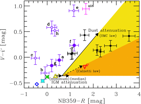
Rest UV two-colour diagram for z≃ 3.1 LyC-emitting galaxies. The vertical axis, V−i′, indicates non-ionizing UV spectral slope, and the horizontal axis, NB359 −R, indicates LyC-to-UV flux density ratio. The filled circles with error bars are the three LAEs without line offset and the open circles with error bars are the five LAEs with line offset. The squares with error bars are LBGs reported in Iwata et al. (2009). The plus mark with error bars is an AGN emitting LyC found in this study. The intrinsic colours of stellar population models are shown by diamond (model D in Table 4), asterisk (C), x-marks (large: B1; small: B2), triangles (large: A1; small: A2) and inverse triangles (large: Ac1 with 100 Myr; small: Ac2 with 100 Myr). The two horizontal arrows show IGM minimum and median attenuations for z = 3.1. The two diagonal arrows show dust attenuations with E(B−V) = 0.1 for the SMC law (solid arrow) and the Calzetti law (dashed arrow). The shaded regions indicate the regions explained by the stellar population model A1 with a combination of IGM and dust attenuations.
5.1 Stellar population models
In order to interpret the UV colours of the LyC-emitting LAEs, we construct models of spectral energy distributions (SEDs) of galaxies. The SED of pure stellar populations depends on metallicity, initial mass function (IMF), star formation history and age. Since we are dealing with LAEs (and LBGs), we consider subsolar metallicities: Z = 1/5 Z⊙ and 1/50 Z⊙. In addition, we consider two more metallicities: Z = 1/2000 Z⊙ (EMP) and 0 (metal-free). SEDs for the former two metallicities are generated by the population synthesis code starburst99 version 5.1 (Leitherer et al. 1999). Those for the latter two are taken from Schaerer (2002, 2003). The IMF is basically assumed to be Salpeter's one (Salpeter 1955): ϕ(m)dm∝mpdm with p=−2.35. Additionally, we consider an extremely top-heavy case with p=−0.1. The mass range of the IMF is assumed to be mup = 100 M⊙ and mlow = 1 M⊙ for Z = 1/5 Z⊙ and 1/50 Z⊙ cases but to be mup = 500 M⊙ and mlow = 50 M⊙ for the EMP and metal-free cases. The average stellar masses are 3.1 M⊙, 48 M⊙ or 111 M⊙ depending on the IMF. We consider an age of 1 Myr after an instantaneous star formation or 10 Myr to 1 Gyr of constant star formation. Table 4 is a summary of the models and their parameters.
Models of stellar population and SED.
| Model | Z/Z⊙ | p | mup | mlow | 〈m〉 | SF history | Age | SED reference |
| A1 | 1/50 | −2.35 | 100 M⊙ | 1 M⊙ | 3.1 M⊙ | Instantaneous | 1 Myr | starburst99 (v.5.1) |
| A2 | 1/5 | −2.35 | 100 M⊙ | 1 M⊙ | 3.1 M⊙ | Instantaneous | 1 Myr | starburst99 (v.5.1) |
| Ac1 | 1/50 | −2.35 | 100 M⊙ | 1 M⊙ | 3.1 M⊙ | Constant | 10, 100, 1000 Myr | starburst99 (v.5.1) |
| Ac2 | 1/5 | −2.35 | 100 M⊙ | 1 M⊙ | 3.1 M⊙ | Constant | 10, 100, 1000 Myr | starburst99 (v.5.1) |
| B1 | 1/50 | −0.1 | 100 M⊙ | 1 M⊙ | 48 M⊙ | Instantaneous | 1 Myr | starburst99 (v.5.1) |
| B2 | 1/5 | −0.1 | 100 M⊙ | 1 M⊙ | 48 M⊙ | Instantaneous | 1 Myr | starburst99 (v.5.1) |
| C | 1/2000 | −2.35 | 500 M⊙ | 50 M⊙ | 111 M⊙ | Instantaneous | 1 Myr | Schaerer (2003) |
| D | 0 | −2.35 | 500 M⊙ | 50 M⊙ | 111 M⊙ | Instantaneous | 1 Myr | Schaerer (2003) |
In Fig. 6, the intrinsic (i.e. no dust and IGM attenuations) colours of the stellar population models are shown by diamond (metal-free: model D); asterisk (EMP: model C); x-marks (extremely top-heavy IMF but normal subsolar metallicity: models B1 and B2); triangles (normal IMF and subsolar metallicity: models A1 and A2); and inverse triangles (normal IMF and subsolar metallicity but constant star formation: models Ac1 and Ac2). NB359 −R colours of the three LAEs without line offset (large filled circles) and LBGs (small squares) seem to be explained by a model with normal IMF and metallicity (models A and Ac). However, the IGM attenuation makes NB359 −R redder as described in the next subsection.
5.2 IGM attenuation
Since the IGM attenuation, especially for the LyC, has a stochastic nature, we estimate the amount based on a Monte Carlo simulation by Inoue & Iwata (2008) (hereafter II08). These authors assumed an empirical distribution function of the intervening absorbers in redshift, column density and Doppler parameter spaces which was derived from the latest observational statistics of that time. Their simulation reproduces the Lyα depressions at z = 0–6 very well.
The LyC opacity is mainly determined by the Lyman limit systems (LLSs; clouds with log10(NH i/cm−2) ≥ 17.2); we compare in Fig. 7 the number density evolution adopted in II08 with new survey results that appeared after the paper. We find that the observational data are not converged yet; Prochaska, O'Meara & Worseck (2010) obtained a smaller number of LLSs at z < 4 than obtained by Péroux et al. (2005) and Songaila & Cowie (2010). We also find that the simulation by II08 adopted a number density tracing the upper bounds of observations. In order to match the new observations, we have reduced the LLS number density, while keeping the number densities of Lyα forest and damped Lyα systems almost intact.4 The updated number density evolution is shown by diamonds in Fig. 7. The new number density of LLSs at z = 2.9 which attenuate the NB359 flux of z = 3.09 sources is about 60 per cent of the previous one.
![The number density evolution of Lyman limit systems which have log10(NH i/cm−2) ≥ 17.2. Observational data are the filled circles (Péroux et al. 2005), squares (Songaila & Cowie 2010) and triangles [Prochaska et al. 2010; a factor of 1.1 larger than their Table 4 which are the density for log10(NH i/cm−2) ≥ 17.5]. Monte Carlo simulations are shown by the open circles (Inoue & Iwata 2008) and the diamonds (updated version).](https://oup.silverchair-cdn.com/oup/backfile/Content_public/Journal/mnras/411/4/10.1111/j.1365-2966.2010.17851.x/2/m_mnras0411-2336-f7.jpeg?Expires=1750246385&Signature=mcbl-y7NUuqgMtrHRAlGMd0hWJjIWmKwkbXup4zpKdGbnZAs9sxCmr1rv2iGsZK5JWa0WxqYhm0lAldvrLGRhmTc7Pc5NSpFN1-QPHoxo~3vMKqhVVPUFOweoAguBTnktRFB0UZ3XLjJZPFSsC1OZ9hGQRp7suiXbI~rhZTAYecBsDm90JoZTeAgTqew9Tq574ef6ba7JVrwjTczrNasPFN0sGPTokw6mp94lHE6h8pgDKslDaYMEIFc2h8LC6zW2gO6o1UmIzjxIfQAe0roKI23wkLdbmn-W5N3U1CjSShLVOeevun5NX7wFgXNlSTqa0Qyoc~78DQsow53TeHzlw__&Key-Pair-Id=APKAIE5G5CRDK6RD3PGA)
The number density evolution of Lyman limit systems which have log10(NH i/cm−2) ≥ 17.2. Observational data are the filled circles (Péroux et al. 2005), squares (Songaila & Cowie 2010) and triangles [Prochaska et al. 2010; a factor of 1.1 larger than their Table 4 which are the density for log10(NH i/cm−2) ≥ 17.5]. Monte Carlo simulations are shown by the open circles (Inoue & Iwata 2008) and the diamonds (updated version).
Fig. 8 shows the cumulative probability of the IGM attenuation through the NB359 for sources at z = 3.09 which is the typical redshift of our LAEs (and LBGs). To estimate the attenuation, we have assumed a constant source spectrum in fν unit. The effect of the different shape of the spectrum is negligible because the wavelength coverage in NB359 is narrow. As can be seen in the figure, the updated version (solid line) is expected to be a much smaller attenuation than the original II08 (dashed line). The median attenuation is reduced from 1.08 to 0.60 mag. Thus, the LLS number density has a significant impact on the expected IGM attenuation. We also find that the attenuation of the smallest 0.15 per cent (e.g. smaller 3σ excess for Gaussian) is 0.35 mag (II08) or 0.28 mag (updated). These attenuations are realized on a line of sight without LLS at z≃ 3 and are produced by numerous and unavoidable Lyα absorption lines in a Lyα forest. Because the update of the number density of absorbers is small for the Lyα forest, the reduction of the smallest attenuations is small. We adopt the attenuation at the cumulative probability of 0.15 per cent as the minimum IGM attenuation in the following.
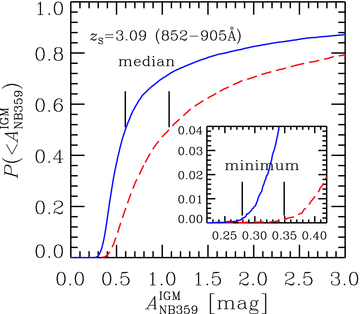
The cumulative probability to have an IGM attenuation in NB359 for z = 3.09 sources smaller than that in the horizontal axis, based on our Monte Carlo simulations: the dashed line (Inoue & Iwata 2008) and the solid line (updated version). The number of realizations of lines of sight is 10 000. The narrow-band filter NB359 captures 852–905 Å in the rest frame of the sources. The inset shows a close-up of the smallest attenuation.
In Fig. 6, we show the minimum and median IGM attenuations by short and long horizontal arrows. Note that the IGM attenuations for other bands in Fig. 6 are either zero (for R and i′) or negligibly small (for V). Table 5 gives a summary of the IGM attenuation.
A summary of reddenings by IGM and dust for a source at z = 3.09.
| Colour excess | E(NB359 −R) | E(V−i′) | |
| IGM | Smallest 0.15 per cent | 0.28 | – |
| (updated) | Median | 0.60 | – |
| Dusta | Calzetti | 0.90 | 0.20 |
| SMC | 0.20 | 0.84 |
| Colour excess | E(NB359 −R) | E(V−i′) | |
| IGM | Smallest 0.15 per cent | 0.28 | – |
| (updated) | Median | 0.60 | – |
| Dusta | Calzetti | 0.90 | 0.20 |
| SMC | 0.20 | 0.84 |
aThese colour excesses correspond to E(B−V) = 0.1 in the rest frame.
5.3 Dust attenuation
If galaxies contain dust, they are reddened. Let us assume two types of dust attenuation law: the Calzetti law (Calzetti et al. 2000) and the extinction law of the Small Magellanic Cloud (SMC). The former attenuation law was derived from spectra of local UV-selected starburst galaxies (Calzetti et al. 2000) and is routinely assumed in studies of high-z galaxies. However, recent studies for z = 2–3 LBGs suggest that an attenuation law steeper than the Calzetti one is favourable for some cases (Reddy et al. 2006; Siana et al. 2009). Thus, we also adopt the SMC law which is the steepest among the known attenuation/extinction laws. We use the model given by Weingartner & Draine (2001) which reproduces the empirical SMC extinction law very well.
The Calzetti law is originally only for λ≥ 1200 Å (Calzetti et al. 2000). However, we simply extrapolate the original formula for λ < 1200 Å. This could be justified by the study of Leitherer et al. (2002) up to λ = 970 Å (but see also Buat et al. 2002) and also be justified by the model of Weingartner & Draine (2001) which does not show any breaks or features up to about 700 Å for graphite and astronomical silicate (Draine & Lee 1984). Table 5 gives a summary of the dust reddenings.
In Fig. 6, we show the region that can be explained by a model with normal subsolar metallicity and IMF and with a combination of dust and IGM attenuations. While a half of LBGs are found in the region, all the LAEs are out of it. We need a new model to explain these LAEs.
5.4 Models with escaping nebular Lyman continuum
Paper I has proposed the importance of an additional contribution by escaping nebular LyC. For an escape of the stellar LyC, the ionized nebulae should be ‘matter-bounded’, at least along some lines of sight, from which we can also expect an escape of nebular LyC produced by the recombination process. Paper I shows that this escaping nebular LyC makes a peaky spectral feature just below the Lyman limit, which we call Lyman limit ‘bump’ (see figs 3 and 4 in Paper I). In fact, our NB359 filter exactly captures this Lyman limit bump at z≃ 3.1. Let us compare this scenario with the observed strength of LyC.
Fig. 9 shows how the Lyman limit bump makes the colour of NB359 −R blue; the colour becomes bluer when a fraction of LyC is absorbed by nebulae and re-emitted in the Lyman limit bump than when all of the LyC escapes. Indeed, the bluest colour is realized when about 40 per cent of the LyC is absorbed (i.e. the escape fraction is about 60 per cent), irrespective of the stellar population model. Based on Fig. 9, we find that moderate subsolar metallicity and normal IMF (solid line: model A1) cannot reach NB359 −R < 0.4 (0.7) for the minimum (median) IGM attenuation even if we consider the additional contribution by nebular LyC. On the other hand, some z≃ 3.1 LAEs detected in LyC show a much bluer colour. Furthermore, even the LAEs with NB359 −R≥ 0.4 are also difficult to explain because their V−i′ is much redder than expectated from their NB359 −R as shown in Fig. 6.
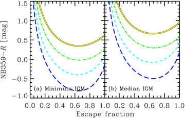
NB359 −R colour for z = 3.1 galaxies, which corresponds to the strength of the Lyman limit ‘bump’, as a function of the escape fraction of stellar LyC. (a) minimum IGM attenuation case and (b) median IGM attenuation case. The curves are the models with escaping nebular LyC: the long-dashed curve for model D in Table 4; the short-dashed curve for model C; the dot–dashed curve for model B1; and the solid curve for model A1. The nebular gas temperature is assumed to be 1 × 10⁴ K.
Figs 10–12 show the two-colour diagrams, same as Fig. 6 but with escaping nebular LyC models. In each panel, the curve with symbols shows the colour sequence as a function of the escape fraction of the stellar LyC. We have assumed the minimum IGM attenuation for the curves. The symbols indicate the colours when the escape fraction is 1.0 (i.e. pure stellar colour + minimum IGM), 0.1 or 0.01. As the escape fraction decreases, NB359 −R colour first becomes bluer than the stellar one due to the Lyman limit bump as shown in Fig. 9, and then, the colour turns over when the escape fraction is about 0.6 and becomes redder and redder after the bluest point. At the same time, the V−i′ colour becomes redder than the stellar one because of the nebular continuum by two-photon and bound–free processes. The amount of these colour changes depends on the strength of the stellar LyC: larger changes by stronger LyC.
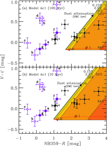
Same as Fig. 6 but a comparison with the escaping nebular LyC scenario of a continuous star-forming galaxy with Z = 1/50 Z⊙ (model Ac1). (a) age from the onset of star formation of 100 Myr and (b) 10 Myr. The dotted curves indicate colour sequences as a function of the escape fraction of stellar LyC with the minimum IGM attenuation. The symbols indicate the positions with the escape fraction of 1.0, 0.1 or 0.01. The shaded regions indicate the regions explained with a combination of IGM and dust attenuations. From thin to thick, the cumulative probability to have the amount of the IGM attenuation increases. The SMC extinction law is adopted for the dust attenuation as shown by the solid arrow. The nebular gas temperature is assumed to be 1 × 10⁴ K.
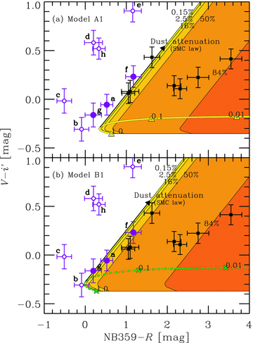
Same as Fig. 10 but the cases of a very young (1 Myr) stellar population with Z = 1/50 Z⊙. (a) normal IMF (model A1; solid line with triangles) and (b) extremely top-heavy IMF (model B1: mean stellar mass of ∼50 M⊙; dot–dashed line with crosses).
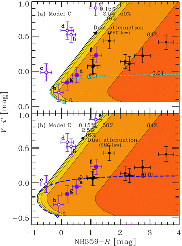
Same as Fig. 10 but the cases of a very young (1 Myr) and massive (∼100 M⊙) stellar population with (a) Z = 1/2000 Z⊙ (model C; short-dashed line with asterisks) and (b) Z = 0 (model D; long-dashed line with diamonds).
The shaded region in each panel of Figs 10–12 shows the colours explained by a combination of IGM and dust attenuations for a specific stellar population model. The thickness of the shades indicates the cumulative probability of the IGM attenuation: higher probability, thicker. We have assumed the SMC extinction law for the dust attenuation but the Calzetti law cases are included in the shaded regions, like in Fig. 6.
Fig. 10 shows the cases of the normal stellar population with a constant star formation (Ac1 in Table 4). We have assumed Z = 1/50 Z⊙, very low, but sometimes observed metallicity (hereafter we call it normally subsolar). The case with Z = 1/5 Z⊙ is always redder in NB359 −R than the case with Z = 1/50 Z⊙. We find that all the LAEs (filled and open circles) and half of the LBGs (squares) cannot be explained even with the duration of the star formation of 10–100 Myr which is younger than a typical age of LBGs (∼300 Myr; Shapley et al. 2003). Therefore, we conclude that the LyC-emitting LAEs should have a stellar population much younger than 10 Myr or much more massive than the standard Salpeter IMF.
Fig. 11 shows the cases of very young (age of 1 Myr) stellar populations with Z = 1/50 Z⊙, normally subsolar metallicity. The case with Z = 1/5 Z⊙ is about 0.2 mag redder in NB359 −R than the present case. Assuming the standard Salpeter IMF [panel (a); model A1], we find that it is still difficult to explain all the LAEs. On the other hand, if we assume an extremely top-heavy IMF whose mean mass is about 50 M⊙[panel (b); model B1], the LAEs without line offset (filled circles) can be explained with an attenuation smaller than the median. However, it is still difficult to explain the LAEs with line offset (open circles). We may have a few true LyC emitters in the five objects because we have statistically rejected the possibility that all the five have a faint foreground object accounting for the NB359 flux in Section 4.2.2. There is another difficulty with model B1. The critical metallicity for the change in IMF from standard to top-heavy, Zcr≲ 10−3 Z⊙ (Bromm & Loeb 2003; Schneider et al. 2003, 2006), is expected to be much lower than Z = 1/50 Z⊙ which is assumed in model B1. Thus, a very massive IMF under the relatively ‘high’ metallicity in model B1 is unlikely. Then, we conclude that it is difficult to explain the strength of LyC of the LAEs with normally subsolar metallicity unless the critical metallicity for the IMF change is much higher than expected in the literature.
Fig. 12 shows the cases of very young (age of 1 Myr) and massive (∼100 M⊙) stellar populations with Z = 1/2000 Z⊙[EMP; model C; panel (a)] and Z = 0[Pop III; model D; panel (b)]. In these cases, we can expect a very massive IMF according to the critical metallicity scenario (Bromm & Loeb 2003; Schneider et al. 2003, 2006). With model C, we can easily explain the three LAEs that are confirmed to be true LyC emitters, whereas the LAEs with line offset are still difficult to be confirmed as such, except for the object b. The Pop III case (model D) can explain objects b and c, and marginally explain e and h. Object d is still difficult but this object shows the largest offset of the Lyα (Table 2), and thus, the foreground probability is the highest. On the other hand, object c shows the smallest offset and is the most likely object as a real LyC emitter among the five offset LAEs. Interestingly enough, the Pop III model can explain the object with a 1–20 per cent smallest IGM attenuation. In summary, very young (∼1 Myr) and massive (∼100 M⊙) EMP stars can reproduce the observed colours of the three LAEs without line offset, and Pop III stars can even reproduce the colours of most of the LAEs with line offset. Because a few line-offset LAEs are likely to be the real LyC emitters, we conclude that the Pop III model is the most favourable stellar population for the LyC-emitting LAEs.
5.5 Models with two stellar populations
The previous subsection shows that the LAEs detected in LyC by I09 are likely to contain a primordial stellar population such as massive Pop III or EMP stars. But how much an amount of these exotic stars is required in them? Also, are Pop III stars really compatible with a slight dust attenuation which is required to explain some LAEs with line offset and red in V−i′ in Fig. 12? To address these questions, let us consider a system in which a primordial stellar population and a normal stellar population with subsolar metallicity and Salpeter IMF coexist. We assume that the normal population makes stars with a constant rate; model Ac2 in Table 4 is adopted for this population. For the primordial population, we adopt model D (Pop III). The stellar mass of the normal population is defined as the multiple of the star formation rate and the duration; we omit the loss of the stellar death for the sake of simplicity. The mass fraction of the primordial population in the total stellar mass is a parameter for the mixture. The contribution of nebular continuum in LyC and in other wavelengths is taken into account for both populations but with different escape fractions: 0.5 for the primordial population and 0.01 for the normal population.5 The normal population may exist in dusty environment, but the primordial population is likely to be dust-free. We adopt two dust attenuation laws: the SMC extinction law and the Calzetti attenuation law as described in Section 5.3 only for the normal underlying population.
The required mass fraction of the primordial stellar population depends on the duration of the star formation in the underlying normal population. This is because the mass of the primordial population, which is required to explain the blue colour of NB359 −R, does not change very much because the colour is determined mainly by the primordial population, while the mass of the underlying population is proportional to the duration. For example, we consider 100 Myr as a duration for z = 3 galaxies (e.g. Shapley et al. 2003). The results are shown in Fig. 13. For other durations, the primordial mass fraction is roughly estimated by an inverse relation to the durations of the underlying star formation. Although we assumed the median IGM attenuation in Fig. 13, the readers can shift all the model curves along the horizontal axis for other IGM attenuations.
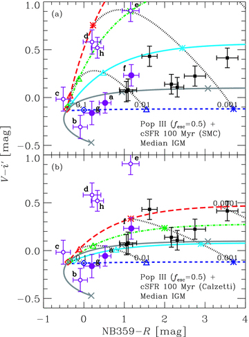
Same as Fig. 6 but comparisons with models of two stellar populations: the cases with models D (Pop III) and Ac2 (underlying population with a subsolar metallicity, 1/5 Z⊙, and a normal IMF) in Table 4. A constant star formation of 100 Myr is assumed for the underlying population. The SMC extinction law is assumed for panel (a) but the Calzetti attenuation law is assumed for (b). The median IGM attenuation is assumed for both the panels. The short-dashed curves are the sequences of the colour as a function of the mass fraction of Pop III stars for dust-free underlying stellar population. The solid, dot–dashed and long-dashed curves are the same sequences but for dusty underlying population with E(B−V) = 0.1, 0.2 and 0.3, respectively. Note that the Pop III stars are assumed to be always dust-free. The positions for the mass fraction of 0.1, 0.01, 0.001 and 0.0001 are indicated by dotted curves with squares, triangles, asterisks and plus-mark, respectively. For Pop III stars, the contribution of escaping nebular LyC is taken into account, assuming the escape fraction of 0.5. The colour sequence with other escape fractions is shown by the triple-dot-dashed curve as in Fig. 12. For the underlying population, the escape fraction of 0.01 is assumed.
The LAEs without offset (objects a, f and g; filled circles in Fig. 13) require a primordial mass fraction of 0.1–10 per cent depending on the IGM and dust attenuations as well as the star formation duration. The dust attenuation for the underlying population is modest as E(B−V) = 0–0.1 for the SMC case or up to 0.3 for the Calzetti case, which is reasonable for z∼ 3 LAEs (e.g. Gawiser et al. 2006). The bluest LAEs (objects b and c; open circles) require a primordial mass fraction of more than 10 per cent, but we could not reject the possibility that their NB359 flux was foreground contamination individually (Section 4.2). The LAEs which are red in V−i′ (objects d, e and h; open circles) can be explained by a model with the SMC law and a small amount of attenuation as E(B−V) ≃ 0.2–0.3 and with a primordial mass fraction of about 0.1 per cent. When the Calzetti law is adopted, the red LAEs require a large amount of dust attenuation as E(B−V) > 0.5 which may be too large. Note that the possibility that the NB359 fluxes of these objects, especially d and e, are foreground contamination is the largest because of the largest line offset (Section 4.2).
The LBGs from which I09 reported detections of LyC (filled squares) are found in the range of the primordial mass fraction of 0.01–1 per cent depending on the dust attenuations. Thus, only a very small amount of primordial stars can account for the observed LyC of these galaxies. On the other hand, some of these LBGs can be explained by a normal population with a large escape fraction of ∼0.5 as shown in Figs 10 and 11. Therefore, the primordial stars are not mandatory for them.
6 SUMMARY AND DISCUSSIONS
We have investigated the nature of the LAEs at z≃ 3.1 detected in our deep narrow-band NB359 imaging with Subaru/S-Cam. The NB359 captures LyC from z > 3. Thus, we detect LyC from the LAEs if they are at z≃ 3.1. These LAEs are special because of their surprisingly strong LyC relative to non-ionizing UV (I09). Deep follow-up spectroscopy with VLT/VIMOS and Subaru/FOCAS for eight such LAEs presented in Section 3 shows that at least three of them are highly likely to be at z≃ 3.1 and the NB359 captures truly their LyC (Sections 4.1.1 and 4.1.2). From the spectra of the three LAEs, we have derived the rest-frame EW of Lyα which are not very large as expected from primordial stellar population models such as Pop III stars. We have also derived upper limits on the He ii λ1640 emission line which are not strict enough to reject Pop III star formation (Table 3). Other five out of the eight LAEs show a 0.8 arcsec offset between the Lyα emission and the continuum detected in NB359 (Fig. 1). For these LAEs, we could not determine the redshifts of the continuum sources (Section 4.2.1). However, it is statistically difficult that all the five have foreground contamination which explains the NB359 detections (Section 4.2.2). Thus, NB359 may capture LyC from a few of the five LAEs with line offset.
Very interestingly, all the LAEs reported by I09 are too bright in LyC to be explained by normal stellar population models (Fig. 6). Although we reduced IGM opacity to match the latest LLS statistics (Figs 7 and 8), compared to the previous estimate, this is true even for the three LAEs which are confirmed to be at z≃ 3.1. Unlike traditional spectral models of galaxies, Paper I proposed a new model taking an escape of nebular LyC into account. This model expects a strong flux excess just below the Lyman limit: we call it Lyman limit ‘bump’. We tried to explain the observed strength in LyC of the LAEs with this new Lyman ‘bump’ model. As a result, we have found that the colour of the LAEs cannot be explained by the stellar population with the standard Salpeter IMF and normally subsolar metallicity (Z≥ 1/50 Z⊙) even with the Lyman ‘bump’ (Figs 10 and 11a). If we assume a very young (∼1 Myr) stellar population with an extremely top-heavy IMF (mean mass of ∼50 M⊙) and Z = 1/50 Z⊙, the three LAEs without line offset can be explained with a relatively smaller IGM attenuation but other five LAEs with line offset cannot be explained yet (Fig. 11b). Because (1) a few of the line-offset LAEs are possibly to be real LyC emitters and (2) the expected critical metallicity for a top-heavy IMF is much lower than the assumed Z = 1/50 Z⊙, we reject this model. This suggests that the LAEs contain a significant amount of ‘primordial’ stars such as EMP or Pop III stars.
A very young (∼1 Myr) and massive (∼100 M⊙) EMP model can reproduce the observed colours of one line-offset LAE as well as the LAEs without offset (Fig. 12a). A Pop III model (∼1 Myr and ∼100 M⊙) can reproduce all but one LAEs discussed here (Fig. 12b). The last LAE (object d) shows the largest offset between NB359 position and Lyα, thus, the possibility of a foreground contamination in NB359 is the highest. Finally, we conclude that the Pop III model is the most favourable stellar population for the LyC-emitting LAEs although the EMP model may be still compatible. If we consider a combination of two stellar populations, ‘primordial’ and ‘normal’ subsolar metallicity with dust, the UV two-colour diagram of all the LAEs and LBGs can be well explained (Fig. 13). In this case, the mass fraction of the ‘primordial’ stars is estimated to be 0.1–10 per cent or more for LAEs with V−i′ < 0.3, about 0.1 per cent for LAEs with V−i′ > 0.3 (but these may be foreground contamination), and 0.01–1 per cent for LBGs, depending on the age of the galaxies, dust content and IGM attenuation (Fig. 13). We also note that the LBGs can be explained by normal stellar populations, and EMP or Pop III stars are not mandatory for them.
The Lyman ‘bump’ galaxies presented in this paper is a new population of high-z galaxies. Indeed, they were missed in standard ‘drop-out’ surveys because they are not ‘drop-out’ but have an excess flux in LyC: Lyman ‘bump’. Because we started from a sample selected based on a narrow-band excess by the Lyα emission line, we did find another excess in LyC. However, Steidel, Pettini & Adelberger (2001) and Shapley et al. (2006) started from an LBG sample, i.e. ‘drop-out’ sample, and thus, they could not find any galaxies with a Lyman ‘bump’. This new population of galaxies probably often emits a strong Lyα emission because they should intrinsically emit strong LyC although a half of the LyC may directly escape. Therefore, starting from an LAE sample selected by a narrow band would be the best to sample the Lyman ‘bump’ galaxies. On the other hand, if all the LAEs had Lyman ‘bump’, i.e. no ‘drop-out’, LAEs and LBGs would separate well. However, a significant fraction of LBGs in fact overlap with LAEs (e.g. Shapley et al. 2003; Noll et al. 2004; Verhamme et al. 2008). This may imply that the fraction of LAEs having Lyman ‘bump’ is small although the IGM attenuation may play a role to hide the Lyman ‘bump’ and to make ‘drop-out’.
A caveat is the lack of confirmation of the Lyman limit ‘bump’ in spectroscopy. Our argument of finding the Lyman limit ‘bump’ is only based on narrow-band photometry. We should confirm the feature in spectroscopy in future.
6.1 A possible evolutionary scenario of Lyman ‘bump’ galaxies
The model with two stellar populations shown in Fig. 13 simultaneously reproduces the strength of the Lyman limit ‘bump’ and non-ionizing UV slope of the LAEs and LBGs detected in LyC by I09. In the model, we have assumed that a primordial stellar population which is dust-free coexists with ‘normal’ stars with subsolar metallicity and dust. We here discuss a possible scenario which may justify this assumption. Fig. 14 shows a schematic picture of the scenario.
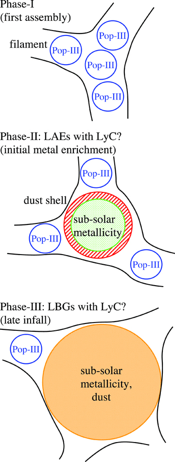
Schematic picture of an evolutionary scenario of Lyman ‘bump’ galaxies.
The hierarchical structure formation scenario argues that a galaxy is assembled from many subgalactic minihaloes. Cosmological hydrodynamics simulations have shown that the galaxy assembly occurs through cosmic filaments and galaxies reside at nodes of the filaments (e.g. Bromm et al. 2009). Greif et al. (2008) examined the first galaxy assembly at z∼ 10 and found that in a 5 × 10⁷ M⊙ halo, ∼10 very massive metal-free stars, the so-called Population III.1, were formed before the assembly. As a radiative feedback by the Pop III.1 stars, pristine gas which was ionized once by the Pop III.1 stars can be more abundant in H2 and HD than before, cool more efficiently and form intermediate-mass metal-free stars, the so-called Population III.2 (e.g. Yoshida et al. 2007). As a result, Greif et al. (2008) expected that gas infalling on to the central part of a galaxy in the potential well likely forms Pop III.2 during the assembly if the gas remains primordial. The Pop III.1 and III.2 stars emit intense LyC which produces cosmological H ii and He iii regions. The escape fraction of LyC is expected to be very high (60–90 per cent; Kitayama et al. 2004; Yoshida et al. 2007) and the nebular LyC can make a significant Lyman limit ‘bump’ (Phase I).
While very massive Pop III.1 may become blackhole directly and make no contribution to the metal enrichment, Pop III.2 stars will end their life with core-collapse supernovae (SNe) and enrich the surrounding gas with metal (e.g. Heger et al. 2003). At the same time, dust grains are also formed by the SNe (e.g. Nozawa et al. 2003). The metal and dust enrichment starts from the central part of the galaxy where the mode of star formation changes into the ‘normal’ mode (e.g. Schneider et al. 2006). If the multiple SNe blast waves make a supershell which contains dust grains, the dust attenuation becomes a screen geometry in which the dust attenuation law is determined only by dust optical properties. If the dust properties resemble the SMC which is also making an intense star formation, the reddening law has a steep wavelength dependence like the SMC extinction law which is assumed in the upper panel of Fig. 13. On the other hand, primordial gas and Pop III stars may be still infalling on to the galaxy from the IGM. These infalling primordial stars can make a significant Lyman limit ‘bump’ (Phase II).
As the star formation proceeds in the main part of the galaxy, dust and metal are mixed well in the ISM. In such a medium, the wavelength dependence of the dust attenuation law becomes weak and expected to be similar to the Calzetti law (Fischera, Dopita & Sutherland 2003; Inoue 2005) which is assumed in the lower panel of Fig. 13. Even in this late stage, a small portion of the surrounding IGM may remain primordial if the metal enrichment in the IGM is not efficient. The primordial gas may form Pop III stars during its infalling process through a cosmic filament (Phase III).
With this scenario, we can explain the two-colour diagram as follows; the LAEs correspond to Phase II (or possibly Phase I). If the age of the galaxies is 10–100 Myr, the primordial mass fraction is ∼1–10 per cent or more in some cases. The amount of the dust attenuation for the underlying population is E(B−V) = 0–0.3. The LBGs correspond to Phase III because of their relatively large stellar mass (∼1010−11 M⊙). If the age is 100–1000 Myr, the primordial mass fraction is <1 per cent and typically ∼0.1 per cent. The amount of the dust attenuation is E(B−V) = 0–0.3 which is similar to LAEs but the attenuation laws may be different from each other.
We can also explain another observational fact: spatial displacements of LyC and non-ionizing UV of the LBGs found in I09. As shown in fig. 2 of I09, the LyC-detected position coincides with a substructure found in the periphery of the main component of the LBGs, although some of these LyC-emitting spots might be foreground contaminations (Vanzella et al. 2010a). In our scenario, we expect that primordial stars emitting LyC exist in the periphery of the galaxies (see also Tornatore et al. 2007). This is exactly the finding from the LBGs by I09. We also expect that LAEs show a smaller offset between LyC and non-ionizing UV than LBGs. According to I09, the offsets of the LAEs are not significant, and thus, smaller than those found in the LBGs. Again, this is consistent with our scenario.
On the other hand, we have found another spatial displacement between the continuum emission, including LyC and Lyα emission lines in some LAEs. While the continuum may not come from the LAEs but from foreground objects, the probability that all the LAEs with line offset have a foreground contamination is very low, as seen in Section 4.2.2. We have also proposed a possible mechanism to produce such a line offset in Section 4.2.3: the LAEs are composed of several unresolved substructures which have different Lyα EWs. This mechanism may fit in our scenario as follows: in Phase II, the continuum including LyC comes from substructures in the periphery and Lyα emission comes from the dusty central component, because the Lyα transmission can be higher than the continuum transmission if the dust is confined to clumps in the supershell (Neufeld 1991).
6.2 Primordial stars at z∼ 3 and intergalactic metal enrichment
Massive (∼100 M⊙) EMP or Pop III stars exist in z∼ 3 LAEs if our interpretation is correct. Since these primordial stars are short-lived (a few Myr) because of their mass, pristine gas should remain to form them until z∼ 3. This argument is not consistent with a scenario of global metal enrichment by Pop III stars at a very early epoch (Mackey, Bromm & Hernquist 2003), in which the entire Universe was enriched to a metallicity floor as Z > 10−3 Z⊙ by Pop III stars at z > 20. On the other hand, recent studies suggest inhomogeneous metal enrichment in the IGM and an extended epoch of Pop III star formation as described below.
Observations of metal absorbers in high-z QSO spectra show that metal enrichment in a Lyα forest is inhomogeneous (Simcoe, Sargent & Rauch 2004; Becker, Rauch & Sargent 2009). For example, Simcoe et al. (2004) show that ∼30 per cent of lines of sight at z∼ 2.5 have metallicity lower than the detection limit of Z∼ 10−3 Z⊙. Cosmological hydrodynamics simulations also show that metal enrichment in the IGM proceeds in a very inhomogeneous way and that a significant volume in the IGM remains pristine until a lower redshift occurs (Tornatore et al. 2007; Oppenheimer, Davé & Finlator 2009; Trenti et al. 2009; Wiersma et al. 2009; Maio et al. 2010). For example, Oppenheimer et al. (2009) show that only ∼1 per cent volume in the IGM is enriched to Z > 10−3 Z⊙ by z = 5. Therefore, IGM metal enrichment is likely to proceed in a patchy way and we can expect a significant chance to form EMP or metal-free stars from pristine materials kept until z∼ 3 (Tornatore et al. 2007; Johnson 2010). In this sense, our argument of the discovery of EMP or metal-free stars at z∼ 3 is consistent with recent studies of IGM metal enrichment.
Our LAEs which may contain primordial stars reside in a massive protocluster region, SSA22 field (Steidel et al. 1998; Hayashino et al. 2004). This field is very peculiar in an enhanced activity of LAEs/LABs (M04), dusty sub-mm galaxies (Tamura et al. 2009) and AGNs (Lehmer et al. 2009). Such activities may proceed IGM metal enrichment efficiently by metal-rich outflows which are observed ubiquitously around LBGs (Steidel et al. 2010). On the other hand, the LAEs' clustering in this field is very low (Hayashino et al. 2004) and this indicates that the LAEs do not lie in the high-density peak of the protocluster but in the less dense periphery of the large-scale filaments (Shimizu, Umemura & Yonehara 2007). The metal enrichment may not proceed well yet there. However, the exact three-dimensional distribution of the LAEs and other types of galaxies by spectroscopy is not obtained yet and is an interesting future work.
6.3 Implications for ionizing background and reionization
The existence of massive EMP or Pop III stars in LAEs may have an impact on the studies of ionizing background and reionization. Based on the observed cosmic evolution of ionizing background, Inoue, Iwata & Deharveng (2006) have suggested a higher LyC emissivity (or escape fraction) of galaxies at higher z. Such an evolving LyC emissivity is supported by galactic LyC observations (Shapley et al. 2006; Bridge et al. 2010; Siana et al. 2010) and simulations (Razoumov & Sommer-Larsen 2006, 2010) and is favourable for the cosmic reionization (Bolton & Haehnelt 2007). On the other hand, the physical mechanism of the evolving LyC emissivity is still uncertain. Some radiative transfer simulations suggest that less massive galaxies have a larger escape fraction of LyC (Razoumov & Sommer-Larsen 2010; Yajima, Choi & Nagamine 2010). Vanzella et al. (2010c) have found a possible luminosity dependence of the LyC emissivity from a large LBG sample. If such less massive galaxies are common at higher z, the global LyC emissivity becomes larger at higher z. Another possibility is that galaxies at higher z have a higher mass fraction of massive EMP or Pop III stars and their LyC emissivity is intrinsically higher. In Section 5.5, we have shown that the primordial mass fraction in the LAEs (1–10 per cent) is more than an order of magnitude larger than that in the LBGs (0.1 per cent). If this larger primordial mass fraction is true for general LAEs and if the LAE population is more common at higher z as found by Ouchi et al. (2008), the galactic LyC emissivity becomes higher at higher z. Of course, these two scenarios can be combined: the less massive LAE population has larger intrinsic LyC emissivity due to primordial stars and larger escape fraction. Indeed, to make a strong Lyman ‘bump’, we need a large escape fraction of ∼0.5 (Paper I). Therefore, such less massive Lyman bump galaxies may play a significant role in the cosmic reionization at z > 6.
We recently found that the spectrum of the object g was taken with Subaru/FOCAS previously (Yamada et al., in preparation).
If each object has a foreground with a probability p, the probability to have k foregrounds among n objects is  (Vanzella et al. 2010a). If we make a subsample of m(≥k) objects including the k foregrounds and we randomly select i objects from the m objects, the probability to have j(≤i, k) foregrounds among the i objects is
  . Since k can vary from j to m−i+j, the total probability to have j foregrounds among i objects becomes
  .
.
There was a revision of zero-points in V, R and i′ after publication of I09 and the resultant shifts in the two-colour diagram as follows: Δ(NB359 −R) =+0.1 and Δ(V−i′) =+0.1. Although the zero-point revision is almost settled, we conservatively apply additional systematic uncertainties of 0.1 mag to the error bars of the observed points by the quadratic combination with statistical uncertainties in photometry.
This is realized only if we change three parameters among the 10 in the empirical distribution function of absorbers. The change is  to (500, 1.7, 1.2), where
  is the normalization of the number of absorbers, and β1 and β2 are the indices of the double power-law for the column density distribution. Note that we should keep the number density of Lyα forest because the Lyα decrements by II08 agree excellently with observations.
In addition to the photoionized gas, we can consider the free–free radiation from hot gas produced by SNe and stellar winds. We have assumed the total energy of the hot gas radiation to be 5 and 1 per cent of the bolometric stellar luminosities for the primordial population (as done in Paper I) and the normal population (Leitherer et al. 1999), respectively. The hot gas temperature is assumed to be 1 × 10⁶ K. However, this hot gas contribution is negligible, as shown in fig. 3 of Paper I.
We are grateful to Jean-Michel Deharveng for suggestions, discussions and encouragements; to Hisanori Furusawa for cooperation in the Subaru observations (S07B-010); and to Eros Vanzella, Masami Ouchi, Masao Mori, Hidenobu Yajima, Masakazu Kobayashi, Hiroshi Shibai and Toru Tsuribe for discussions and comments. We thank the anonymous referee for her/his comments which helped us improve the content of this paper. AKI is supported by KAKENHI (the Grant-in-Aid for Young Scientists B: 19740108) by The Ministry of Education, Culture, Sports, Science and Technology (MEXT) of Japan and by the Institute for Industrial Research, Osaka Sangyo University. In the early phase of this work, AKI was invited to the Laroratoire d'Astrophysique de Marseille and financially supported by the Observatoire Astronomique de Marseille-Provence.
REFERENCES
Author notes
This work is based on data collected with the Subaru Telescope operated by the National Astronomical Observatory of Japan (programme ID: S07B-010 and S08B-046) and with the Very Large Telescope operated by the European Southern Observatory, Chile (programme ID: 081.A-0081).
