


Abstract
We present a study characterizing the environments of galaxies in the redshift range of 0.4 < z < 1 based on data from the POWIR near-infrared imaging and DEEP2 spectroscopic redshift surveys, down to a stellar mass of log M*= 10.25 M⊙. Galaxy environments are measured in terms of nearest-neighbour densities as well as fixed aperture densities and kinematical and dynamical parameters of neighbour galaxies within a radius of 1 h−1 Mpc. We disentangle the correlations between galaxy stellar mass, galaxy colour and galaxy environment, using not only galaxy number densities, but also other environmental characteristics such as velocity dispersion, mean harmonic radius and crossing time. We find that galaxy colour and the fraction of blue galaxies depends very strongly on stellar mass at 0.4 < z < 1, while a weak additional dependence on local number densities is in place at lower redshifts (0.4 < z < 0.7). This environmental influence is most visible in the colours of intermediate-mass galaxies (10.5 < log M* < 11), whereas colours of lower- and higher-mass galaxies remain largely unchanged with redshift and environment. At a fixed stellar mass, the colour–density relation almost disappears, while the colour–stellar mass relation is present at all local densities. We find a weak correlation between stellar mass and environment at intermediate redshifts, which contributes to the overall colour–density relation. We furthermore do not find a significant correlation between galaxy colour and virial mass, i.e. parent dark matter halo mass. Galaxy stellar mass thus appears to be the crucial defining parameter for intrinsic galaxy properties such as ongoing star formation and colour.
1 INTRODUCTION
The influence of environment on the properties of galaxies and their evolution has become evident over the last three decades. Among the early evidence for an environmental effect on galaxy evolution was the discovery of the morphology–density relation (Oemler 1974; Dressler 1980), showing that morphologies of cluster galaxies are not randomly distributed, but they depend on the distance from the cluster centre, or alternatively on the local density in which a galaxy resides. Another early study by Davis & Geller (1976) showed that the two-point correlation function, measured using a catalogue of preferentially selected field galaxies, depends on galaxy morphology. We have since learned that not only galaxy morphology depends on environment, but also the mean age of a galaxy's stellar population is affected: galaxies in low-density environments appear on average 1–2 Gyr younger than their counterparts in high-density environments like galaxy clusters, or local overdensities in galaxy groups (Thomas et al. 2005; Clemens et al. 2006). This was also shown by Bernardi et al. (1998), who found that among a population of early-type galaxies, field ellipticals tend to present populations about 1 Gyr younger than those in clusters. Recently, Cooper et al. (2010) found evidence for a correlation between age and environment at fixed stellar mass, such that galaxies in higher-density regions formed earlier than galaxies of similar mass in lower-density environments. Similar evidence comes from studies of galaxy clustering. Skibba & Sheth (2009) analysed the correlations between galaxy colours and the environment using marked correlation functions and argued that, in order to explain the observed colour dependence, a significant fraction of faint satellite galaxies must be blue. Skibba et al. (2009) argued that much of the correlations between morphologies and the environment are explained by the colour–environment correlation.
On the other hand, the star formation histories, colours and morphologies of galaxies are very sensitive to galaxy stellar mass (see e.g. Brinchmann & Ellis 2000; Jimenez et al. 2005; Thomas et al. 2005): the higher the stellar mass of a galaxy the earlier, shorter and more intense the initial burst of star formation. The peak in the star formation activity then shifts to lower-mass galaxies as cosmic time proceeds (see e.g. Bundy et al. 2006). The relative importance of the various factors in shaping the galaxies that we observe today is unclear. What are the roles of stellar mass, total galaxy mass and parent dark matter halo mass? What has a stronger influence, local density or membership in a massive structure? Is being a ‘satellite’ or a ‘central’ galaxy an important factor, as recently suggested by e.g. van den Bosch et al. (2008) and Skibba (2009)?
There is considerable previous work addressing these questions. Blanton et al. (2005) showed that most environmental correlations can be explained by two galaxy properties, colour and luminosity, and that correlations with structural properties are less important. Clemens et al. (2006) find that metallicity and α-enhancement are independent of environment, but correlate with galaxy velocity dispersion, i.e. the galaxy's dark matter halo mass. On the other hand, Blanton et al. (2006) argue that galaxy properties are only related to the mass of its parent dark matter halo, i.e. the total mass of the structure in which a galaxy resides. Weinmann et al. (2006) similarly emphasize the importance of group halo mass. They furthermore find that the properties of satellite galaxies are strongly correlated with those of their central galaxy. Kauffmann et al. (2004) find that galaxy structure depends strongly on stellar mass, while star formation history is very sensitive to local density. Recently, Bamford et al. (2009) showed the presence of a morphology–density relation at fixed stellar mass using Galaxy Zoo morphologies. However, they do not find a dependence of morphology on group mass, either determined from the velocity dispersion or the integrated group light.
Looking at higher redshifts (z ∼ 1), the correlations found in the local Universe seem to be either already in place or reversed. A strong dependence of galaxy colours on local projected number density was found by Cooper et al. (2006) up to z ∼ 1. Cucciati et al. (2006) on the other hand find that the colour–density relation present at 0.25 < z < 0.60 progressively disappears until it is undetectable at z ∼ 0.9. The morphology–density relation was found to be already in place at z ∼ 1 over a wide range of densities from cluster cores to the field (Postman et al. 2005; Smith et al. 2005). Stellar mass seems to set an upper limit to this density dependence: Tasca et al. (2009) found that above M*∼ 1010.8 M⊙ morphology does not evolve or depend on environment up to z ∼ 1, a result confirmed by Iovino et al. (2010). They also argue that the lower fraction of blue galaxies in groups with respect to the field is mainly caused by luminosity-selected samples biased towards blue low-mass galaxies. The colour difference largely disappears when stellar mass selected samples are used. The relation between SFR and local density at high z is controversial too. The SFR–density relation found for SDSS galaxies locally seems to be reversed at higher redshifts: Elbaz et al. (2007) and Cooper et al. (2008) find galaxies with higher SFR are located in higher densities at z ∼ 1. However, the opposite was found by Patel et al. (2009), who observe the same strong decline of SFR with density at z ∼ 0.8 as in the SDSS.
The contradictory results of the above studies may be partly due to the problematic and manifold definitions of what a galaxy environment is, and how to quantify it. The options include (1) group or cluster membership, compared to the rather ill-defined ‘field’ (2) local number densities, based on number counts in a fixed aperture, or the distance to the nth nearest neighbour, where both, the choice of aperture size or n, introduce an arbitrary element; and (3) the dark matter halo mass, based on halo occupation models.
Galaxy stellar mass itself, usually regarded as an intrinsic property of a galaxy, may also depend on environment, as suggested by the stellar mass–halo mass correlation (see e.g. Moster et al. 2010). Massive elliptical galaxies are often found in the cores of galaxy clusters, or at high local densities, while lower-mass spirals are located on the outskirts of larger structures or in small groups, as is our Local Group. However, this traditional view is not necessarily always the case: massive ellipticals are also found in the field (e.g. Colbert, Mulchaey & Zabludoff 2001), and low-mass galaxies with elliptical morphology are found preferentially in high local densities (e.g. Roberts et al. 2007). It is hence not clear if, and how, a galaxy's stellar mass depends on the environment and how this dependence evolves with redshift.
High-redshift studies have additional problems: deep surveys usually cover a small area, suffering from the problem of cosmic variance. Another issue is the limited availability of spectroscopic redshifts. Photometric redshifts, even quite accurate ones, make it difficult to accurately define environments since they smear out structures along the line of sight. This is especially problematic at low densities (Cooper et al. 2005).
We approach this problem with the combination of a deep infrared survey covering a large field of view, the POWIR survey, and the DEEP2 redshift survey providing the spectroscopic redshifts for a large number of objects. Additionally, our galaxy sample is selected in the K-band. The near-infrared bands are a much better proxy for stellar mass than optical bands, since they are sensitive to the light of old, low-mass stars and less sensitive to the effects of dust. Optical colours correspond to rest-frame UV light, which traces young and hot stellar populations, and thus is more sensitive to star formation than stellar mass. The near-IR selection therefore corresponds to a selection based on stellar mass rather than star formation. This allows us to study correlations with stellar mass without the colour bias of optical luminosity selected samples (Conselice et al. 2008).
Section 2 describes the two surveys and the resulting samples used in this study. The ways in which we characterize a galaxy's environment is explained in Section 3. Section 4 presents our results, Section 5 discusses their implications and Section 6 summarizes our most important findings. We assume the standard ΛCDM cosmology and a flat universe with ΩΛ = 0.73, ΩM = 0.27 and a relative Hubble constant h = H0/100 is used.
2 THE SAMPLE
2.1 The POWIR and DEEP2 surveys
This study is based on data obtained by the Palomar Observatory Wide-Field Infrared (POWIR) survey described in Conselice et al. (2008). The goal of this survey is to construct a K-band selected and stellar mass limited sample covering a large field of view, and containing a large number of galaxies with spectroscopic redshifts. The POWIR survey covers four fields: the Extended Groth Strip (EGS, Davis et al. 2007) and three additional fields subsequently referred to as Field 2, 3 and 4. All four fields have been observed by the DEEP2 (Deep Extragalactic Evolutionary Probe) redshift survey (Davis et al. 2003).
Deep J- and Ks-band imaging was obtained with the WIRC camera on the Palomar 5-m telescope. The survey consists of 75 pointings covering an area of ∼1.5 deg2 with an average 5σ depth reaching down to Ks,vega = 20.2. For a detailed description of the observations and data reduction procedures see Bundy et al. (2006). The corresponding optical data come from the 3.6-m Canada–France–Hawaii Telescope (CFHT) using the CFH12K camera. Imaging in the bands B, R and I was taken, reaching a 5σ depth of RAB = 25.1. The details of these observations and their reduction are given in Coil et al. (2004). The seeing is comparable in the infrared and optical data (FWHM ∼ 1 arcsec). All photometry was measured within a 2-arcsec diameter aperture.
Spectroscopic redshifts were obtained with the Keck DEIMOS spectrograph (Faber et al. 2003) as a part of the DEEP2 redshift survey (Davis et al. 2003). Targets were selected down to RAB < 24.1 independent of their colour in the EGS field, whereas in fields 2, 3 and 4 targets were additionally selected based on (B − R) and (R − I) colour, focusing on selecting galaxies at z > 0.7. The spectroscopic sampling rate is about 60 per cent in all four fields. Together with the spectroscopic success rate of ∼70 per cent this yields an overall spectroscopic completeness of ∼40 per cent in all four fields over a redshift range of 0.4 < z < 1. The different target selection criteria in fields 2, 3, 4 and the EGS lead to an overall smaller number of galaxies in the redshift interval 0.4 < z < 0.7, since objects in this range come mainly from the EGS field. This redshift interval thus has a smaller surveyed volume relative to the higher redshift range of 0.7 < z < 1.
The photometric catalogue of galaxies detected in the Ks-band images with the SExtractor package (Bertin & Arnouts 1996) was then matched to the DEEP2 redshift catalogue. The matching between the R-band selected redshift catalogue and the K-band selected photometric catalogue was done within a 1-arcsec radius. This results in a very low rate of spurious matches of 1–2 per cent due to the low surface densities in both catalogues (Bundy et al. 2006; Conselice et al. 2008). The spectroscopic sample is magnitude limited at RAB = 24.1 due to the DEEP2 target selection limit, whereas the Ks-band selected photometric catalogue has a magnitude limit of RAB = 25.1. This leads to a lower percentage of galaxies with spectroscopic redshifts [∼22 per cent, see Conselice et al. (2007)] in the photometric catalogue than the spectroscopic completeness of 40 per cent quoted above. For all galaxies in the Ks-band selected photometric sample, which have no measured spectroscopic redshift, we measure photometric redshifts. This procedure is described in the following section. For a more detailed description of the sample selection and an extensive discussion of the completeness we refer the reader to Conselice et al. (2007).
2.2 Additional photometric redshifts
The spectroscopic redshift sample is complemented by photometric redshifts measured from the optical and IR photometry described above. For galaxies that meet the spectroscopic target selection, but were not observed due to instrumental constraints, the neural network code annz (Collister & Lahav 2004) was used. This includes all galaxies brighter than RAB = 24.1, which either were not sampled spectroscopically (∼40 per cent of galaxies in our catalogue with RAB = 24.1) or have no reliable spectroscopic redshift measurement (∼30 per cent of spectroscopically observed galaxies). This sample of galaxies without spectroscopic redshifts (∼60 per cent of the total Ks-band selected sample) cover the same magnitude range as galaxies with spectroscopic redshift, which can therefore be used at a training set for the annz neural network code. Photometric redshifts of galaxies fainter than RAB = 24.1 were measured with the bpz package (Benítez 2000), which uses a Bayesian approach, including information about the likelihood of a certain redshift–brightness combination, taken from the distribution of galaxies in the Hubble Deep Field (Benítez 2000). bpz is well suited for determining photometric redshifts of faint galaxies, for which no comparison sample with spectroscopic redshifts is available.
The photometric redshift accuracy is good out to z ∼ 1.4 with an uncertainty of Δz/(1 + z) = 0.07 (Conselice et al. 2007). For a detailed description of the photometric redshift estimates we refer the reader to Conselice et al. (2007, 2008) and Bundy et al. (2006). The number of galaxies in the full sample (spectroscopic redshifts plus additional photometric redshifts) and the spec-z sample (secure spectroscopic redshifts only) are as follows: the full sample has 50 119 galaxies, while the spec-z sample comprises 10 682 galaxies.
2.3 Stellar mass measurements
Stellar masses were estimated by fitting the optical and near-infrared photometric data points with synthetic spectral energy distributions (SEDs) from Bruzual & Charlot (2003) spanning a variety of galaxy ages, metallicities and star formation histories. We use an exponentially declining star formation history with an e-folding time between 0.01 and 10 Gyr and ages of the star formation onset between 0 and 10 Gyr. The metallicities span a range of 0.0001–0.05. The typical uncertainties of the model SED fitting is ∼0.1–0.2 dex. Adding to this the photometric errors yields a total stellar mass uncertainty of 0.2–0.3 dex. We note that for intermediate-age stellar populations the stellar masses can be systematically overestimated. However, as shown in Conselice et al. (2007), for the present sample the masses are lower only by an average of 0.07 dex, when using models with AGB-TP stars. Another source of systematic error is the choice of IMF. Here, the IMF of Chabrier (2003) is used. The details of the stellar mass measurements are fully described in Bundy et al. (2006).
Bundy et al. (2006) and Conselice et al. (2007) also estimate the completeness limits in stellar mass from the Ks-band detection limit at different redshifts by placing model galaxies at the high-redshift end of each redshift bin. For a redshift of z ∼ 1 they find that the full sample (including galaxies with photometric redshifts) is 100 per cent complete down to a stellar mass of log M* = 10.25. Galaxies down to this stellar mass and redshift limit are detected independently of their colour. Our sample is therefore not strongly biased towards bluer galaxies at high z. We use a stellar mass limit of log M* = 10.25 and a redshift limit of z = 1 throughout this paper.
Out of the 50 119 galaxies in our whole catalogue 14 563 are above the stellar mass limit log M* > 10.25 and below the redshift limit z ≤ 1 and hence are included in this study. 4101 of these galaxies have spectroscopic redshifts. The final full sample therefore has 14 563 galaxies, and the spec-z sample has 4101 galaxies.
2.4 Rest-frame (U − B) colours and colour fractions fblue, fgreen and fred
Rest-frame (U − B) colours were derived by Willmer et al. (2006) in the Vega magnitude system. All magnitudes and colours used in this paper are converted into the AB magnitude system. The transformation between the Vega and AB system is a linear shift given by the AB magnitude of Vega in the respective filter. The (U − B) colours used in this study can be transformed in the following way: (U − B)AB = (U − B)Vega+ 0.83 (Willmer et al. 2006).


Fig. 1 shows the colour limits in the colour–magnitude diagram in three redshift bins. The red line corresponds to the red sequence of Willmer et al. (2006), while the green line shows the limit blueward of which galaxies are considered to lie in the green valley. Galaxies below the blue line are considered blue cloud systems.
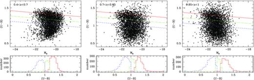
Colour–magnitude diagram (CMD) of the full sample (14 563 galaxies) in three redshift bins. The red (solid) line indicates the location of the red sequence found by Willmer et al. (2006), while the green (dotted) and blue (dashed) lines are the limits below (bluer than) which galaxies are considered green and blue, respectively. The small panels below each CMD shows the colour distribution of blue, green and red galaxies.
3 CHARACTERIZATION OF GALAXY ENVIRONMENTS
This section describes the different environment measures we use in this study. We use two different approaches: the first one is based on measuring the distance to the nth nearest neighbours of each galaxy within a redshift slice, while the second one uses all galaxies within a certain physical radius and radial velocity interval.
3.1 Nearest-neighbour densities
Cooper et al. (2007) measured the third nearest-neighbour densities of galaxies in the DEEP2 sample, which we utilize here. The choice of n for nth nearest-neighbour distances was found to have a weak influence on the resulting density values (Cooper et al. 2005). Cooper et al. (2005) also investigated possible effects of the selection function of the DEEP2 survey and concluded that it does not introduce any environmental bias, at least up to z ∼ 1.
The method used to determine the nearest-neighbour densities is fully described in Cooper et al. (2006, 2007). Only galaxies with spectroscopic redshifts are used in measuring local densities. First the projected distance D3 to the third nearest neighbour within a radial velocity window of ±1000 km s−1 is measured. This is then converted into a surface density Σ3 = 3/(πD23). To account for different sampling rates of the DEEP2 survey at different redshifts, Σ3 is divided by the mean surface density 〈Σ3〉 into slices of Δz = 0.04. This yields the relative overdensity (1 +δ3), which is not affected by redshift-dependent incompleteness. Note that the ratio Σ3/〈Σ3〉 is denoted not by δ3, but by (1 +δ3). δ3 itself is the overdensity defined as (Σ3−〈Σ3〉)/〈Σ3〉. Using log (1 +δ3) is convenient for separating the sample into over- and underdense regions: if log (1 +δ3) is positive, the galaxy is located in an overdense region, while a negative log (1 +δ3) corresponds to an underdense area relative to the mean density at each redshift.
To minimize edge effects, we exclude galaxies closer than 1 h−1 Mpc to a survey border. Out of the 4101 galaxies in the spectroscopic redshift sample, 486 galaxies are within the 1 h−1 Mpc border region and excluded from further analysis. The sample used in the local density analysis then consists of 3615 galaxies.
3.2 Environment within a fixed aperture
In addition to the nearest-neighbour densities, which are expressed as relative overdensities, the absolute local density for each galaxy is calculated by counting neighbouring galaxies within a certain fixed radius (or aperture), and a fixed radial velocity interval. This search radius is chosen to be 1 h−1 Mpc, which gives the best correlation (as we will show below) between the number of neighbours, their velocity dispersion and the parent dark matter halo mass based on Millennium Simulation (Springel et al. 2005). We show this by using a light-cone catalogue produced from the full simulation within a box of 500 h−1 Mpc on each side. The dark matter haloes are populated with galaxies according to the halo occupation distribution (HOD) models of Skibba & Sheth (2009). Galaxy luminosities are computed according to the model described in Skibba et al. (2006). The light-cone catalogue is fully described in Skibba & Sheth (2009). It comprises positions, distances and magnitudes for 954 212 simulated galaxies down to an absolute magnitude limit of Mr − 5 log h =− 19. The distances include the peculiar motions of the galaxies and are converted into radial velocities using the relative Hubble constant h = 1, as it is used in the simulation. The number densities and galaxy velocity dispersion within different fixed apertures of 1, 2 and 5 h−1 Mpc and a velocity window of ±1000 km s−1 are computed. Fig. 2 shows the relation between the measured velocity dispersion of all galaxies within the fixed aperture and velocity interval as a tracer of the halo mass and the halo mass from the simulation itself. The different apertures are shown as blue stars (5 h−1 Mpc), green crosses (2 h−1 Mpc) and red squares (1 h−1 Mpc). The error bars show the 1σ dispersion in each bin. Within an aperture of 5 h−1 Mpc there is no relation between halo mass (MDM) and velocity dispersion (σr): σr has a value of around 500 km s−1 at all halo masses. At 2 h−1 Mpc σr starts to be sensitive to the halo mass, but the relation flattens off at log MDM∼ 13.5 M⊙ and  . Using 1 h−1 Mpc the relation becomes steeper and we are able to trace the parent dark matter halo mass down to ∼ 1012.5 M⊙ or
  (Fig. 2).

Comparison between dark matter halo mass MDM and velocity dispersion σr computed within different circular apertures and a radial velocity interval of Δv =±1000 km s−1. The results for the different apertures are shown as blue stars (5 h−1 Mpc), green crosses (2 h−1 Mpc) and red squares (1 h−1 Mpc). The error bars give the 1σ dispersion in each bin. A small shift in MDM is applied for a better visualization of the error bars.
The radial velocity interval within which neighbouring galaxies are included is set to Δv =±1000 km s−1. This choice may sound arbitrary; however, it is motivated by the distribution of galaxies in our survey: the vast majority of galaxies in the DEEP2 survey are either isolated or located in galaxy groups, not in clusters (Gerke et al. 2007). A velocity of 1000 km s−1 corresponds to the escape velocity of a massive galaxy group with a velocity dispersion of  .
.
From all galaxies found within the fixed aperture and velocity interval we then compute the following quantities:
Radial velocity dispersion σr and the virial mass Mvir as a halo mass estimator;
Harmonic radius RH as a compactness estimator;
Crossing time tc as a dynamical state estimator;
The offset in projection and velocity, relative to the average, R;
Number of neighbours N1 Mpc within 1 h−1 Mpc as a richness estimator.

 denotes the rms deviations in projected distance and peculiar velocity, respectively, of all galaxies within the 1 h−1 Mpc radius. A galaxy with a large distance d from the geometric centre or a large offset from the mean velocity vpec will yield a large value of R while an average galaxy should have
  . A small R then indicates that the galaxy is closer to the centre in space and velocity than the average galaxy, which can be interpreted as being more likely at rest in (or close to) the centre of the potential well of the parent structure or dark matter halo.
4 RESULTS
In the following we present our results in two ways, comparing the full sample (zspec and zphot combined) and for galaxies with secure spectroscopic redshifts only. The photometric redshifts are not suited to compute dynamical quantities, since the typical uncertainties of Δz/(1 + z) ∼ 0.03 are much larger than the typical velocity dispersion of galaxy groups. However, for comparison reasons we plot the obtained values next to the ones obtained by using spectroscopic redshifts only in Figs 4 and 5. As described in Section 2 our sample consists of galaxies down to a stellar mass of M* = 10.25 up to a redshift of z = 1. To avoid edge effects, galaxies with a distance from the border of the surveyed field of less than 1 h−1 Mpc were excluded in the following analysis. First we compare the two local density estimators, N1 Mpc and (1 +δ3) as described in Section 3, then we describe the evolution of the environmental characteristics (σr and Mvir, RH, tc, R and N1 Mpc) and the rest-frame colours with cosmic time. We then investigate the correlation between colours and fraction of red, green and blue galaxies with local density, halo mass and stellar mass. And finally, to disentangle the influence of stellar mass and local density on galaxy colour, the sample is split in different bins of stellar mass and local density.
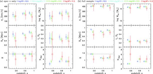
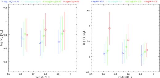
Environmental properties of galaxies at different stellar masses as a function of redshift. Left side: spectroscopic redshifts only; right side: full sample. Note that velocity-related quantities measured with the full sample (including galaxies with photometric redshifts) are not reliable measurements and we show them only for comparison reasons. Top left: radial velocity dispersion σr; top right: virial mass log Mvir; mid-left: harmonic radius RH; mid-right: crossing time in units of the Hubble time tcH0; bottom left: R parameter, the dotted line shows the average value of  (see text); bottom right: number of galaxies N1 Mpc. The sample is sliced into four stellar mass and three redshift bins. The stellar mass bins are colour coded: red circles (log M* > 11.5), green stars (11.5 ≥ log M* > 11), cyan boxes (11 ≥ log M* > 10.5) and blue triangles (log M* < 10.5). The redshift bins are 0.4 ≤ z < 0.7, 0.7 ≤ z < 0.85, and 0.85 ≤ z < 1. The data points in each bin are offset in redshift direction for clarity. The error bars represent the 3σ error of the mean in each bin.
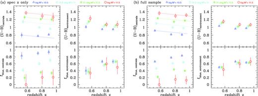
Colours of galaxies with different stellar masses and their environments as a function of redshift. Left side: spectroscopic redshifts only; right side: full sample. Top left: (U − B) colour of ‘central’ galaxies; top right: (U − B) colour of galaxies in the central's environment; bottom left: blue fraction fblue of ‘central’ galaxies; bottom right: blue fraction of galaxies in the central's environment. The sample is sliced in four stellar mass and three redshift bins, as in Fig. 4. The dashed lines trace the expected colour evolution of a passively evolving stellar population formed at high z (see text). The error bars represent the 3σ error of the mean in each bin.
4.1 Richness N1 Mpc versus relative overdensity (1 +δ3)
As described in Section 3, two different methods are used to estimate richness/density: the number of neighbours within a fixed aperture, N1 Mpc, and the nearest-neighbour density, (1 +δ3), based on the distance to the third nearest neighbour, measured by Cooper et al. (2007). The same population of galaxies is used to measure the two local density estimators. Only galaxies with secure spectroscopic redshifts are used when comparing (1 +δ3) with N1 Mpc. Although the two values should roughly agree overall, they trace different things: N1 Mpc is equivalent to an absolute comoving density, while (1 +δ3) is a relative overdensity, i.e. density normalized by the mean density in the galaxy's respective redshift interval (±0.04). The nearest-neighbour density is an adaptive measurement that is well suited to characterize local galaxy concentrations on small scales, which might not be identified as density enhancements by the fixed aperture density. Furthermore, it gives a continuous range of densities, while the fixed aperture density can by construction only have discreet values, increasing the intrinsic uncertainty of the measurement. On the other hand, the nth nearest-neighbour density is more sensitive to interlopers, since due to the variable area, the resulting density can change significantly due to the presence of a single object, especially when a small n is used.
We decided not to convert N1 Mpc into units of Mpc−2 but to leave it in number of galaxies within the aperture. Since the aperture is the same for all galaxies, this has no effect on the results, but allows us to easily determine how many galaxies our results are based upon.
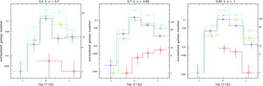
Fig. 3 compares log N1 Mpc with log (1 +δ3) in the three redshift ranges. The two measures agree on average. To quantify the correlation between the two densities we compute Spearman rank correlation coefficients ρ. The value of ρ ranges between −1 ≤ρ≤ 1, where ρ = 1 (ρ=−1) means that the two variables are perfectly correlated (anticorrelated) by a monotonic function. Completely uncorrelated variables result in ρ = 0. Taking into account the sample size in each bin we estimate the significance of the value of ρ using the conversion from correlation coefficient to z-score (Fieller, Hartley & Pearson 1957). The correlation coefficients and their significance in the three redshift bins are ρ0.4−0.7 = 0.31 at ∼3σ, ρ0.7−0.85 = 0.50 at ∼8σ and ρ0.85−1 = 0.44 at ∼7σ. However, in the most over- and underdense environments the linear correlation becomes flatter. This shows that the nearest-neighbour density (1 +δ3) is better suited for tracing the high and low ends of the relative density distribution.
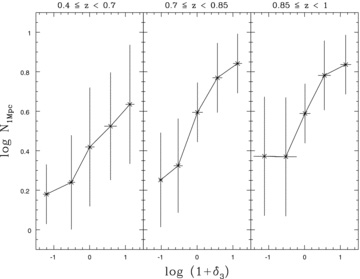
Comparison between relative overdensity log (1 +δ3) and richness log N1 Mpc. The error bars show the 1σ spread in each bin.
4.2 Galaxy environment correlated with stellar mass and cosmic time
The different environmental characteristics, as described in Section 3, are plotted in Fig. 4 as a function of z. Note that all the quantities are measured with galaxies within 1 h−1 Mpc radius and within a radial velocity interval of Δv =±1000 km s−1 as described above. To investigate the evolution of these quantities with redshift, as well as possible differences in the evolution of galaxies of different stellar mass, the sample is split into four stellar mass bins and three redshift bins. These three redshift bins (used throughout the paper) are 0.4 ≤ z < 0.7, 0.7 ≤ z < 0.85 and 0.85 ≤ z < 1. The stellar mass bins are indicated at the top of the figure with the respective colour: log M* < 10.5 in blue, 10.5 < log M* < 11 in cyan, 11 < log M* < 11.5 in green and log M* > 11.5 in red. Table 1 gives the numbers of galaxies as well as the mean values of stellar mass and redshift in each bin of stellar mass and redshift. The sum of the number of galaxies over all bins is lower than the sample size quoted in Section 2, due to galaxies that have no neighbours within the search radius and therefore no measured environmental parameters. These are about 25 per cent of galaxies in the spectroscopic redshift sample and about 20 per cent of galaxies in the full sample.
| (a) | n (M1) | 〈log M*〉 | 〈z〉 | n (M2) | 〈log M*〉 | 〈z〉 | n (M3) | 〈log M*〉 | 〈z〉 | n (M4) | 〈log M*〉 | 〈z〉 |
| z1 | 97 | 10.38 | 0.5802 | 226 | 10.75 | 0.6032 | 116 | 11.18 | 0.6124 | 11 | 11.63 | 0.6062 |
| z2 | 346 | 10.37 | 0.7846 | 740 | 10.76 | 0.7833 | 370 | 11.18 | 0.7864 | 24 | 11.60 | 0.7840 |
| z3 | 239 | 10.37 | 0.9264 | 521 | 10.75 | 0.9202 | 323 | 11.17 | 0.9245 | 16 | 11.62 | 0.9132 |
| (b) | ||||||||||||
| z1 | 1174 | 10.37 | 0.5589 | 1914 | 10.73 | 0.5664 | 602 | 11.18 | 0.5797 | 28 | 11.63 | 0.5815 |
| z2 | 1070 | 10.38 | 0.7802 | 1887 | 10.74 | 0.7799 | 853 | 11.18 | 0.7827 | 54 | 11.61 | 0.7794 |
| z3 | 990 | 10.37 | 0.9248 | 2164 | 10.75 | 0.9241 | 1168 | 11.18 | 0.9294 | 72 | 11.65 | 0.9175 |
Stellar mass bins: M1: log M* < 10.5, M2: 10.5 < log M* < 11, M3: 11 < log M* < 11.5, M4: log M* > 11.5
redshift bins: z1: 0.4 ≤ z < 0.7; z2: 0.7 ≤ z < 0.85; z3: 0.85 ≤ z < 1
| (a) | n (M1) | 〈log M*〉 | 〈z〉 | n (M2) | 〈log M*〉 | 〈z〉 | n (M3) | 〈log M*〉 | 〈z〉 | n (M4) | 〈log M*〉 | 〈z〉 |
| z1 | 97 | 10.38 | 0.5802 | 226 | 10.75 | 0.6032 | 116 | 11.18 | 0.6124 | 11 | 11.63 | 0.6062 |
| z2 | 346 | 10.37 | 0.7846 | 740 | 10.76 | 0.7833 | 370 | 11.18 | 0.7864 | 24 | 11.60 | 0.7840 |
| z3 | 239 | 10.37 | 0.9264 | 521 | 10.75 | 0.9202 | 323 | 11.17 | 0.9245 | 16 | 11.62 | 0.9132 |
| (b) | ||||||||||||
| z1 | 1174 | 10.37 | 0.5589 | 1914 | 10.73 | 0.5664 | 602 | 11.18 | 0.5797 | 28 | 11.63 | 0.5815 |
| z2 | 1070 | 10.38 | 0.7802 | 1887 | 10.74 | 0.7799 | 853 | 11.18 | 0.7827 | 54 | 11.61 | 0.7794 |
| z3 | 990 | 10.37 | 0.9248 | 2164 | 10.75 | 0.9241 | 1168 | 11.18 | 0.9294 | 72 | 11.65 | 0.9175 |
Stellar mass bins: M1: log M* < 10.5, M2: 10.5 < log M* < 11, M3: 11 < log M* < 11.5, M4: log M* > 11.5
redshift bins: z1: 0.4 ≤ z < 0.7; z2: 0.7 ≤ z < 0.85; z3: 0.85 ≤ z < 1
4.2.1 The parent dark matter halo:![formula]() and Mvir
and Mvir
Fig. 4, top row, shows the median σr and Mvir in three redshift bins. The range of velocity dispersions σr is found to be largely similar at all redshifts. There are no significant changes with redshift or stellar mass. The same is seen for the virial mass Mvir. We do not see a significant trend for more massive galaxies to be situated in more massive structures as measured by σr at 0.4 < z < 1, neither do we find obvious indications for a growth of halo mass over time. However, this might be due to the large uncertainties of Mvir due to the generally small numbers of galaxies found (〈N〉 < 10 at all redshifts and masses). The comparison between the spectroscopic sample (left side) and the full sample (spectroscopic plus photometric redshifts, right side) illustrates that photometric redshifts are not suited for this kind of study. The velocity dispersion calculated including galaxies with photometric redshifts is systematically overestimated, with  , as expected for a random distribution of velocities within a ±1000 km s−1 window. The same can be seen for Mvir which is of course related to σr.
4.2.2 Compactness and dynamical state: mean harmonic radius RH and crossing time tc
Fig. 4, middle row, shows the median RH and tc values in three redshift bins. We find that RH does vary slightly with redshift as well as with galaxy stellar mass. There is a trend that more massive galaxies reside in more compact environments, i.e. at lower RH. The typical crossing times tc have large scatters and seem to be largely independent of redshift and galaxy stellar mass. The median tc are of the order of 0.2–0.3 Hubble times, which is consistent with the time-scale in which relaxation can take place (Ferguson & Sandage 1990). There is a trend for more massive galaxies to be located in more relaxed or more dynamically evolved structures, i.e. in structures with a shorter crossing time, however, this trend is only significant in one redshift bin (0.7 ≤ z < 0.85). RH is less affected by the use of photometric redshifts than tc, since it is not velocity related, while tc is measured from the velocity dispersion. RH is only affected by the inclusion of foreground/background galaxies due to the use of photo-z's, while tc is directly affected by the artificially high velocity dispersion in the full sample.
4.2.3 Distribution of galaxies in phase space: the R parameter
The bottom left panel of Fig. 4 shows the evolution of the R parameter with redshift. The most massive galaxies show on average consistently smaller R values than the lower-mass galaxies. They seem to occupy a special position in phase space, although the uncertainties are large due to the small number of galaxies with stellar masses above 1011.5 M⊙. However, the low R suggests that the most massive galaxies sit closer to the centre of their potential well or dark matter halo than an average galaxy in our sample. This result is consistent with what was found for groups dominated by bright ellipticals in the local universe: Zabludoff & Mulchaey (2000) find that the brightest group galaxies (BGGs) are more likely to lie close to the centre of projected space and velocity than the rest of the group population. We find possible redshift evolution in the value of R. Between 0.8 < z ≤ 1 galaxies with different stellar masses are indistinguishable in their position in phase space, while at lower redshifts (z ≤ 0.7) the most massive galaxies with M*≥ 1011.5 M⊙ have R ∼ 1 compared to R ∼ 1.4 for lower-mass galaxies. This difference is significant at about 3σ. Including galaxies with photometric redshifts dilutes the result: now all galaxies are more ‘central’ than galaxies in their environment, but simply because they were selected to be so, and more of the included galaxies around them are random foreground or background objects.
4.2.4 Richness of the structure: number of neighbours N1 Mpc
The average number of neighbours found for each galaxy within our 1 h−1 Mpc and |Δv| ≤ 1000 km s−1 limits are shown in the bottom right panel of Fig. 4. The numbers are similar for galaxies with lower stellar masses (log M* < 11), while the more massive galaxies have generally more neighbours. This trend is most significant (3σ confidence level) for the most massive galaxies, but is also visible for galaxies in the range 11 < log M* < 11.5. Furthermore, the most massive galaxies show increasing numbers of neighbours with decreasing redshift, while for the rest of the galaxies the median number of neighbours is roughly constant with redshift. The same trend can be seen for the relative overdensity log (1 +δ3) which will be discussed later in this paper.
4.3 Rest-frame colours and the blue fraction of galaxies as a function of cosmic time
In the following section we show how the average (U − B) colour and blue fractions change with cosmic time. Fig. 5 shows the evolution of galaxy rest-frame colours and blue fraction with redshift, divided in the same four stellar mass bins as used before. The colours do not evolve strongly with redshift, as already noticed by Willmer et al. (2006). The dotted lines show the expected evolution of (U − B) with redshift for an old passively evolving stellar population taken from van Dokkum & Franx (2000). Each line is adjusted to the low-redshift data point of each stellar mass bin, tracing back the expected colour of passively evolving galaxies at higher redshifts. The expected change is very small and the average colours indeed do not change very much with redshift. However, there is a slight colour evolution, especially for intermediate-mass galaxies (10.5 < log M* < 11). Their mean colour changes from (U − B) ∼ 0.95 at z ∼ 0.9 to (U − B) ∼ 1.15 at z ∼ 0.6. As can be seen in Fig. 5 there is a very strong dependence of (U − B) colour on stellar mass, which we will investigate in more detail in Section 4.5. The same is true for the blue fraction which strongly depends on galaxy stellar mass. The blue fraction fblue increases only slightly with redshift for low- and high-mass galaxies. For intermediate-mass galaxies, however, fblue evolves strongly from 70 per cent at z ∼ 0.9 to 45 per cent at z ∼ 0.6 (see Fig. 5), analogous to the evolution in (U − B).
The mean (U − B) colour and blue fraction of galaxies found in each galaxy's environment are shown in Fig. 5. They are denoted by (U − B)environment and fblue,environment, in contrast to (U − B)centrals and fblue,centrals for the average colour and blue fraction of galaxies in each redshift bin. Note that in this context ‘centrals’ does not imply that these galaxies are the central galaxy of their parent dark matter halo, but is used as distinction to the colour and blue fraction of a galaxy's environment. The environment–colour and blue fraction shows if and how ‘satellite’ galaxies react to the properties (M*, local density) of the central galaxy in their halo. The top right panel of Fig. 5 shows that the mean colour of the environment also depends slightly on the ‘central’ galaxy's stellar mass. Higher-mass galaxies are surrounded by redder neighbours. However, this dependence is much weaker than the primary dependence of a galaxy's colour on its own stellar mass. Since the most massive galaxies are more likely central galaxies, we would expect to see a different behaviour of the environment–colour and environment–blue fraction in the highest M* bin. Examining Fig. 5 it appears this could be the case: environment–colour (and blue fraction) seems to rise (and drop) faster with redshift than the other three lower stellar mass bins. The significance of this difference is about 3σ.
The inclusion of galaxies with photometric redshift does not lead to large changes in the results. Rest-frame colour is not as sensitive to photometric redshift errors as the environmental characteristics discussed above.
4.4 Rest-frame colours and colour fractions correlated with environment
In this section we investigate the dependence of the (U − B) colour and fractions of blue, red and green galaxies on environment, i.e. local density and halo mass. As described above, the nearest-neighbour density (1 +δ3) is a better tracer of the extremes in the density distribution and is therefore used in the following analysis, instead of the aperture density N1 Mpc. The colour–density relation is well studied up to z ∼ 1 (see e.g. Cooper et al. 2006; Cucciati et al. 2006; Iovino et al. 2010) and can be seen as an analogue to the morphology–density relation (see e.g. Dressler 1980). To mimic the separation into different morphological types, we plot the fraction of red, blue and green galaxies, analogous to ellipticals, spirals and S0 galaxies. Colour does not perfectly correspond to morphology, but since we lack the morphological information we take colour as a proxy of morphology.
We also compare the colour and red, blue and green fractions with the virial mass Mvir. The virial mass is computed from the velocity dispersion, which is a good indicator of a galaxy's parent dark matter halo mass (see Section 3 and Fig. 2). The dark matter halo can influence the properties of its galaxies through various processes like ram pressure stripping, harassment, galaxy merging or strangulation. The likelihood of these processes which either enhance or suppress star formation depends on the mass of the halo, where the processes that quench star formation like ram pressure stripping, which is proportional to the density of the intracluster medium and the square of the velocity dispersion (Gunn & Gott 1972), or ‘harassment’ (repeated high-velocity encounters, see e.g. Moore et al. 1996) are occurring in massive dark matter haloes. Galaxy merging, on the other hand, which can trigger star formation preferentially occurs in smaller groups or lower-mass haloes, since cold gas and low relative velocities are required to efficiently trigger star formation (see e.g. Mihos & Hernquist 1994). We would then expect a possible connection between galaxy colour and the mass of its parent dark matter halo, such that higher-mass dark matter haloes are populated by on average redder galaxies. On the other hand, the process of strangulation (Larson, Tinsley & Caldwell 1980), which involves the stripping of hot gas only, could occur in low-mass and high-mass haloes. Skibba (2009) argue that the near-independence of the satellite colour distribution on halo mass may be evidence of strangulation, since it requires a process that occurs independently of halo mass. In this context it is interesting to test if colour and colour fractions show a dependence on virial mass.
4.4.1 (U − B) and fcolour as a function of local density and compactness
First, we investigate the colour–density relation for our entire sample with no stellar mass binning, analogous to other studies of the colour–density relation (Cucciati et al. 2006; Cassata et al. 2007; Cooper et al. 2007) and the morphology–density relation (Postman et al. 2005; Smith et al. 2005). Mean (U − B) colours and the fractions of red, green and blue galaxies are plotted as a function of local density log (1 +δ3) in Fig. 6, top left. There is a dependence of both colour and colour fractions on the local density. The blue fraction fblue decreases from ∼0.65 in underdense environments to ∼0.35 at high overdensity. There is also a related increase of fred with local density, while the fraction of green galaxies fgreen is constant, within the errors. The colour–density relation also evolves with redshift, steepening significantly with later cosmic time. The decrease of fblue with log (1 +δ3) is significant at ∼2σ in the two lower-redshift bins and disappears at z > 0.85. We compute the Spearman rank coefficient ρ to quantify the correlation between (U − B) and log (1 +δ3) in the three redshift bins, yielding the following values: ρ0.4−0.7 = 0.21, ρ0.7−0.85 = 0.14 and ρ0.85−1 = 0.04. Taking into account our sample size in each bin we estimate a significance level of ∼2σ for ρ0.4−0.7 and ρ0.7−0.85 and 0.5σ for ρ0.85−1, i.e. colour and density are uncorrelated at z > 0.85 for log M* > 10.25. This is consistent with the results of Cooper et al. (2006, 2007), who find a strong correlation between red fraction and local density, with the slope of the relation decreasing with look-back time. The significance of the fred–density relation in their colour-limited sample is, however, higher (>3σ) than the significance of the relation we find for our stellar mass limited sample. Gerke et al. (2007) find a similar result for galaxy groups in the DEEP2 survey, such that galaxy groups have lower fractions of blue galaxies than the field. However, this difference is seen up to a higher redshift (z ∼ 1.3) than colour–density relation in our sample. Our result is also consistent with the findings of Cucciati et al. (2006) using the VIMOS VLT Deep Survey (VVDS) to construct a luminosity-limited sample of 6582 galaxies and local densities measured on a larger scale (5 h−1 Mpc) than the densities we use here. Cucciati et al. (2006) find that a clear relation between colour and local density at 0.25 < z < 0.6, which progressively disappears with higher redshift and is not present at z ∼ 0.9, coinciding roughly with the redshift at which the colour–density relation disappears in our sample (z > 0.85).
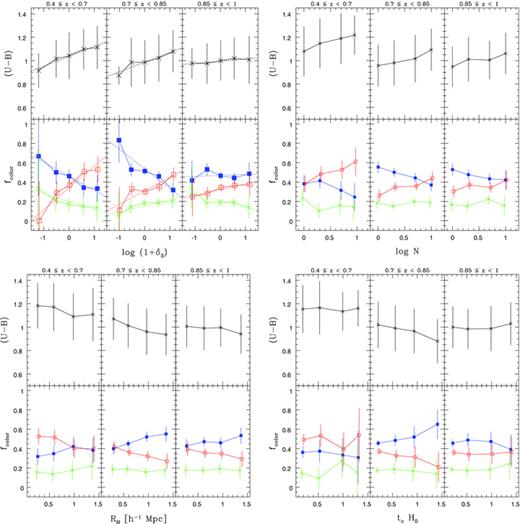
(U − B) colour and the fraction of blue, red and green galaxies as a function of different environmental characteristics in three redshift bins (as in Fig. 4). Top left: nearest-neighbour density log (1 +δ3); top right: number of neighbours log N1 Mpc; bottom left: mean harmonic radius RH; bottom right: dimensionless crossing time tcH0. Each plot is divided in mean (U − B) (top panels) and colour fractions (bottom panels), fblue (blue solid boxes), fred (red open symbols) and fgreen (green crosses). See text for the definition of colour fractions. The error bars represent the 1σ spread in each bin. The dashed lines are least-squares fits to the data points.
Analogous to the relation between (U − B) and (1 +δ3) we find a similar correlation between (U − B) colour and the number of neighbours N1 Mpc. The top right panel of Fig. 6 shows colour and colour fractions as a function of log N1 Mpc. This colour–density relation has a slightly lower significance than the colour–overdensity relation between (U − B) and (1 +δ3) and is also most significant in the lower- and intermediate-redshift bin. We also detect a weak correlation between colour and mean harmonic radius RH, i.e. compactness of the structure. This relation is shown in the bottom left panel of Fig. 6. RH is related to the local density, since galaxies in a high density will most likely have small projected separations. However, a high RH can also be achieved with a low number of galaxies, i.e. at a low density. The colour–compactness relation is similar to the colour–density relation, showing more red galaxies in structures with small RH, most significantly in the intermediate-redshift bin. Its significance is, however, lower than that of the colour–density relation. The bottom right panel of Fig. 6 shows colour and colour fractions as a function of the dimensionless crossing time tcH0. The crossing time and colours are possibly correlated in the intermediate redshift bin, in a way that structures with longer crossing times are populated by bluer galaxies. The significance of the correlation between tc and fblue is ∼1σ.
4.4.2 (U − B) and fcolour as a function of halo mass
In the following the dependence between galaxy colour and parent dark matter halo mass is investigated. Only galaxies with spectroscopic redshifts are used to determine the virial mass of each galaxy's parent dark matter halo. Fig. 7 shows colour and colour fractions as a function of halo mass log Mvir. In contrast to the colour–density relation there is no significant correlation between galaxy colour and log Mvir. The correlation coefficients are <0.1 with a significance of <1σ at all redshifts. However, there is a trend that more massive haloes have slightly bluer central galaxies in the redshift range of 0.7 ≤ z < 0.85. Additionally, fblue decreases faster with redshift at low log Mvir than at high log Mvir. This implies that galaxies in lower-mass haloes become redder earlier. Alternatively, high-mass haloes could accrete more blue field galaxies. However, this trend has only ∼1σ significance. Note that the error bars in the figure are the 1σ rms deviation in each Mvir bin, not the measurement errors, which are negligible compared to the uncertainties due to the on average low number of objects around each galaxy. The virial mass is accurate within a factor of a few (3–5) due to the low numbers of objects we use to determine it (〈N1 Mpc〉∼ 4).
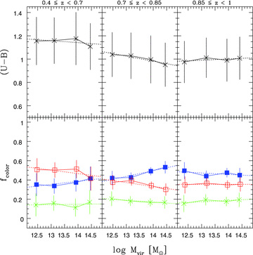
Same as Fig. 6 but for virial mass log Mvir.
4.5 Rest-frame colours and colour fractions correlated with stellar mass
In analogy to the relation between colour and density and colour and halo mass, we now investigate the relation between colour and stellar mass M*. Since no environment measure sensitive to photometric redshift errors or edge effects is used in the following, we use the full sample (> 14 000 galaxies) down to log M* = 10.25 and z = 1.
Fig. 8 shows (U − B) colour and colour fraction as a function of stellar mass (log M*). As can immediately be seen, both colour and colour fractions depend strongly on galaxy stellar mass. The fraction of red galaxies fred changes with M* from ∼0.2 at log M*∼ 10.5 to ∼0.8 at log M*∼ 11.5 at z ∼ 1. The fcolour–stellar mass relation is roughly constant with redshift, flattening slightly at the low-mass end from fred∼ 0.2 at z ∼ 1 to fred∼ 0.3 at z ∼ 0.5. The strong relation between rest-frame colour and a galaxy's stellar mass is the basis of the relation between colour and mass-to-light ratio (M/L) found by Bell & de Jong (2001), which allows stellar masses to be determined from luminosity and rest-frame colours. We compute the significance of the correlation of fblue and fred with stellar mass using the Spearman rank coefficient and its z-score, as already used above for the colour–density and colour–halo mass correlations. The correlation coefficient is ρ∼ 0.4 at all redshifts, corresponding to a significance level of >8σ.
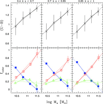
Same as Fig. 6 but for stellar mass log M*.
Interestingly, there are significantly more green valley galaxies at intermediate M*(log M*∼ 11) than in the lowest and highest stellar mass bin at all redshifts. The green fraction changes from fgreen∼ 0.25 at log M*∼ 11 to fgreen∼ 0.15 at log M*∼ 10.5 and log M*∼ 11.5. This difference has a >2σ significance and is roughly constant at all redshifts. This might indicate that the transition from blue to red between 0.4 ≤ z < 1 is happening in intermediate mass galaxies, while it is mostly finished at high stellar masses and has yet to start at low stellar masses.
Our findings are roughly consistent with the results of Iovino et al. (2010) using the zCOSMOS group catalogue of Knobel et al. (2009) reaching up to z ∼ 0.8. Iovino et al. (2010) find that the fraction of blue galaxies reaches ‘saturation’ at the extremes of the stellar mass distribution, i.e. Fblue∼ 1 at low stellar mass (log M*∼ 10) and Fblue∼ 0 at high stellar mass (log M* > 10.6). At intermediate stellar masses the blue fraction varies with environment, being lowest in the group sample and highest in the sample of isolated galaxies. The difference becomes progressively larger at lower redshifts and is most distinctive at 0.25 < z < 0.45. This trend seems to continue towards low redshift, where Kauffmann et al. (2003b), using the SDSS, find that the fraction of galaxies with old stellar populations is rapidly increasing at stellar masses above log M* = 10.3.
4.6 Disentangling dependencies on environment from dependencies on stellar mass
To disentangle the effects of local density and stellar mass on galaxy colours and colour fractions we split the sample into different bins of stellar mass and density (see Figs 9–11). The stellar mass bins are the same as the bins used in Figs 4 and 5: red circles correspond to galaxies with log M* > 11.5, green stars are 11.5 > log M* > 11, cyan squares comprise of galaxies between 11 > log M* > 10.5 and blue triangles are all galaxies below log M* < 10.5, down to the limiting stellar mass of log M* = 10.25. Analogous to the four stellar mass bins, the sample is also divided into four local density bins defined in the following way: red circles are the densest environments with log (1 +δ3) > 0.75, green stars are slightly overdense environments at 0.75 > log (1 +δ3) > 0, cyan boxes are slightly underdense with 0 > log (1 +δ3) > −0.75 and blue triangles are the most underdense environments where log (1 +δ3) < −0.75. Fig. 9 shows the numbers of galaxies in each stellar mass and local density bin. To compare the three redshift ranges we normalize the number of galaxies in each bin by the total number of galaxies in the respective redshift range. The four stellar mass bins are colour coded in the figure as described above, while the density is plotted on the x-axis. This figure shows at which local densities most galaxies of a given stellar mass are found and how this might change with redshift. We find that at intermediate redshifts there are more massive galaxies at higher densities. This redshift range also shows the strongest colour–density relation (see Fig. 6).
Number of galaxies in the four stellar mass bins at different local densities. The stellar mass bins are colour coded and plotted with different symbols as in Figs 10 and 11: blue triangles (log M* < 10.5), cyan squares (10.5 < log M* < 11), green stars (11 < log M* < 11.5) and red circles (log M* > 11.5). The scale of the y-axis on the left side shows the number of galaxies in each stellar mass bin and local density bin, normalized by the total number of galaxies in the respective redshift bin. For comparison reasons we show the number of galaxies in each bin without this normalization on the right-hand side of each plot.
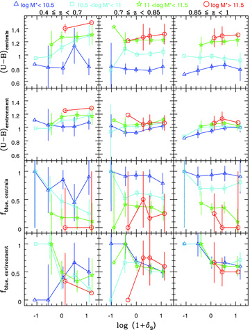
(U − B) colour and the blue fraction of galaxies (fblue,centrals) and their environment (fblue,environment) in different stellar mass bins: (U − B) and fblue as a function of nearest-neighbour density log (1 +δ3) for galaxies in four stellar mass bins. From top to bottom: (U − B) of galaxies, mean (U − B) of the galaxies' neighbours, fblue of galaxies, fblue of neighbours. The stellar mass bins are colour coded and plotted with different symbols: blue triangles (log M* < 10.5), cyan squares (10.5 < log M* < 11), green stars (11 < log M* < 11.5) and red circles (log M* > 11.5). The error bars represent the 3σ error of the mean in each bin.
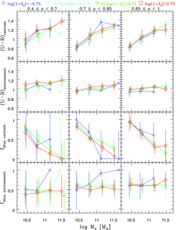
(U − B) colour and the blue fraction of galaxies (fblue,centrals) and their environment (fblue,environment) in different local density bins: (U − B) and fblue as a function of stellar mass log M* for galaxies in four local density bins. From top to bottom: (U − B) of galaxies, mean (U − B) of the galaxies' neighbours, fblue of galaxies, fblue of neighbours. The local density bins are colour coded and plotted with different symbols: blue triangles (log (1 +δ3) < − 0.75), cyan squares (−0.75 < log (1 +δ3) < 0), green stars (0 < log (1 +δ3) < 0.75) and red circles (log (1 +δ3) > 0.75). The error bars represent the 3σ error of the mean in each bin.
Conselice et al. (2007) discuss the evolution of the number densities of the most massive galaxies (log M* > 11.5) in our sample. They show that log M* > 11.5 galaxies are already in place by z ∼ 1 and their number densities do not evolve significantly after that. In Fig. 9 we still see some evolution in the numbers of the most massive galaxies (log M* > 11.5, red circles) between z ∼ 1 and z ∼ 0.8. This evolution is taking place at the highest local densities. The same is seen for galaxies in the next stellar mass bin (11.5 > log M* > 11), which increase in numbers only at the highest relative overdensities. The lowest redshift bin does not have enough volume to probe the number densities of the most massive galaxies, due to their intrinsic rareness. Intermediate- and low-mass galaxies (log M* < 11) also show increased numbers per unit volume at the highest local densities. The number densities of these galaxies are generally increasing between z ∼ 1 and z ∼ 0.8, but the increase is strongest in the most overdense environments.
We use the above stellar mass and local density bins to replot the overall colour–density relation shown in Fig. 6 and the overall colour–stellar mass relation (Fig. 8) in bins of stellar mass and relative density. Figs 10 and 11 then show the same plots as in Figs 6 and 8 but with the data split into bins of relative density and stellar mass. For clarity only the blue fraction is plotted here. In Figs 10 and 11 we also show the colour and blue fraction of the environment, i.e. mean (U − B) of neighbours and fraction of blue galaxies in each galaxy's environment, denoted by (U − B)environment and fblue,environment in contrast to (U − B)centrals and fblue,centrals for colours and blue fractions of individual galaxies. Note again that in this context ‘centrals’ does not imply that these galaxies are indeed the central galaxy of their parent dark matter halo, but is used to distinguish between values for individual galaxies and mean values of neighbouring galaxies.
4.6.1 The colour–density relation in different stellar mass bins
Fig. 10 shows how (U − B) colour and the blue fraction (fblue) of galaxies with different stellar masses depend on local density log (1 +δ3). The top row shows the (U − B) colour of ‘central’ galaxies, and the second row shows the mean (U − B) of the galaxies' environment as already used in Section 4.3. The dependence of colour on density shown in Fig. 6 largely disappears for low stellar mass (log M* < 10.5) and high stellar mass (log M* > 11) galaxies. However, there is a residual colour–density relation for the intermediate mass galaxies (cyan, 11 > log M* > 10.5). This relation is only present in the lowest-redshift bin and disappears completely at z ∼ 0.8. The same is seen for fblue. The strong dependency of colour on stellar mass becomes clear in the plot: the different stellar mass bins are clearly separated in colour. The mean colour of the environment shows the overall colour–density relation and a slight dependence on stellar mass of the ‘central’ galaxy: the most massive galaxies are surrounded by redder galaxies. This trend is weak, but becomes more evident at lower redshifts, where the separation of the different stellar mass bins becomes clearer.
4.6.2 The colour–stellar mass relation in different local density bins
Fig. 11 shows the colour–stellar mass relation in four bins of local density. The colour–stellar mass relation is clearly present in all density bins, but there is almost no colour separation between the different densities, reflecting the disappearance of the colour–density relation described above. The colour–stellar mass relation is very similar at all densities, i.e. independent of local density, especially at high z. At low redshift the highest density bin seems to have a lower blue fraction; however, the dispersion is large due to the small number statistics. The mean colour of a galaxy's environment (U − B)environment is also influenced by the stellar mass of a galaxy, such that more massive galaxies have on average slightly redder companions. This dependence however is not nearly as strong as the colour–stellar mass relation for individual galaxies ((U − B)centrals). The colour difference between log M*∼ 10.5 and 11.5 is  mag, whereas the difference in the environment colour over the same stellar mass range is Δ (U − B)environment = 0.15 mag.
4.6.3 Correlations between density and stellar mass
Above we discussed the relations between galaxy colour and density on one hand and stellar mass on the other as two independent trends. However, how do stellar mass and local density correlate?Fig. 12 shows the dependence of M* on log (1 +δ3). There is a trend that galaxies in higher local densities tend to have higher stellar masses; however, this trend is weak and is only significant in the intermediate redshift bin, with a correlation coefficient ρ0.7−0.85 = 0.2 at a significance of ∼3σ. This redshift bin also shows the strongest colour–density relation. In the other two redshift bins the correlation has a significance of 1.2σ(0.4 ≤ z < 0.7) and 1.5σ(0.85 ≤ z < 1).
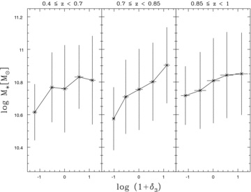
Comparison between relative overdensity log (1 +δ3) and stellar mass log M* in the three redshift bins. The error bars represent the 1σ spread in each bin.
Is the slight redshift evolution of the density–stellar mass relation shown in Fig. 12 due to an evolution of stellar mass at a given density or a change in density at a given stellar mass?Fig. 13 shows the redshift evolution of stellar mass at different local densities (left-hand panel) and the redshift evolution of local density at different stellar masses (right-hand panel). The weak correlation between stellar mass and density is visible; however, the stellar mass at a given density does not evolve with time. The same is true for the evolution of densities at a given stellar mass, apart from the most massive galaxies which show a strong evolution of relative overdensity with time. Their environments change from about average densities to more than 10 times the average, overdense regions. The same increase is seen in the number of neighbours N1 Mpc as discussed earlier (see Fig. 4). This can be explained in terms of dynamical friction: since massive galaxies are more likely to be at the centre of their structure, neighbours are more likely to accumulate in their environment, increasing their local density over time. In our sample we indeed see evidence for the massive galaxies to be more likely located at the centre of mass and velocity of a galaxy association (see discussion of the R parameter in Section 4.2.3).
Evolution of stellar mass and relative overdensity with redshift. Left-hand panel: evolution of stellar mass in different density bins. Right-hand panel: evolution of densities in different stellar mass bins. The relative overdensity of the most massive galaxies increases with redshift. The error bars represent the 1σ dispersion in each bin.
5 DISCUSSION
In the following we discuss the implications of the results presented above and compare them with results from the literature.
5.1 Environments of galaxies with different stellar masses
Overall, we do not find a relation between galaxy stellar mass and radial velocity dispersion of galaxies within the galaxy's environment, or mass of the dark matter halo (as measured by Mvir). This may partly be caused by the high uncertainties in measuring virial masses, due to the intrinsic low number of galaxies in the structures we probe here, possible interlopers or the possibility that some structures are unvirialized. However, as illustrated in Fig. 2, the velocity dispersions we measure are tracing halo masses in the Millennium Simulation down to log MDM∼ 12.5. The lack of a (strong) correlation between stellar mass and virial mass is a challenge for models of hierarchical structure formation, since they expect more massive galaxies to be located in more massive structures (or parent dark matter haloes).
The environmental parameters do not change significantly with redshift, apart from RH, which decreases with redshift at all stellar masses, and R, N1 Mpc and (1 +δ3) for the most massive galaxies (log M* > 11.5). We find that the most massive galaxies tend to be more likely central galaxies (smaller R-parameter). They also move closer to the centre of mass and velocity of the structure, as suggested by a decreasing R with a decreasing redshift. The most massive galaxies are located in the higher absolute local densities (N1 Mpc) as well as in the higher relative overdensities (1 +δ3) and accrete more galaxies over time, both in absolute numbers (N1 Mpc) and relative to the average (1 +δ3). This can be explained by dynamical friction and is in general agreement with the expectations of hierarchical structure formation. The increase in local densities and number of companions might increase the rate at which merging is happening in these structures. Conselice et al. (2007) and Conselice, Yang & Bluck (2009) measure the merger rates for galaxies in our sample from morphological parameters and do not find an increasing merger rate with redshift for massive galaxies. The fraction of distorted ellipticals, however, is increasing in the same redshift range, reaching a maximum of about 30 per cent at z ∼ 0.7 (Conselice et al. 2007), which could be connected to the increasing local densities.
Some of the environmental parameters are connected to intrinsic galaxy properties of colour and stellar mass: we find a correlation between colour and local density, overdensity and compactness, as well as between local density, compactness and stellar mass, as discussed in the following.
5.2 Relations between galaxy colour and stellar mass, local density and halo mass
There is a very strong correlation between galaxy colour and stellar mass (>8σ significance) at all redshifts. This colour–stellar mass relation evolves only slightly with redshift. The stellar mass where red and blue fractions cross over, i.e. where there is an equal fraction of blue and red galaxies, occurs on average at log M*∼ 10.8 and evolves slightly from log M*∼ 10.9 at high z to log M*∼ 10.7 at low z. In the local universe this transition occurs at lower stellar masses: using the SDSS Kauffmann et al. (2003a,b) find a sharp transition from the dominance of blue to red galaxies at log M*∼ 10.3. Our results also agree with the findings of a recent study by Iovino et al. (2010) who investigate the relationship between colour, stellar mass and environment up to z ∼ 0.8. They find a qualitatively similar strong dependence of the blue fraction on stellar mass in all environments studied (groups, field and isolated galaxies).
We find a weak correlation between colour and local density (∼2σ significance) for the whole sample and also a weak correlation between density and stellar mass (∼3σ significance). The colour–density and density–stellar mass relations change in a similar way with redshift: both relations are most significant at intermediate redshifts, and they both disappear at high z. This is in good agreement with previous similar studies (Cooper et al. 2006, 2007; Cucciati et al. 2006; Cassata et al. 2007). Cucciati et al. (2006) find a similar progressive disappearance of the colour–density relation with redshift, even though they use galaxy densities measured on much larger scales of 5 h−1 Mpc. Cooper et al. (2007) however find that a strong relation between colour and local density persists out to z > 1. This might partly be caused by their sample selection, which is rest-frame B-band luminosity limited. We cannot confirm the colour–density relation at z > 0.85 in our K-band selected sample.
If the sample is split up into different stellar mass bins, the colour–density relation disappears completely for the lowest- and highest-mass galaxies, remaining only in the stellar mass range of 10.5 < log M* < 11, although at a lower significance than for the whole sample. We conclude that the overall colour–density relation is powered by these intermediate-mass galaxies, as well as by the fact that there are more low-mass galaxies at lower densities and vice versa. Stellar mass and relative overdensity are not strongly correlated; however, the correlation accounts for most of the colour–density relation seen in our sample. In other words, the colour–density relation is a combination of a strong colour–stellar mass relation and a weak stellar mass–density relation. The strong colour–stellar mass relation is present at all local densities and it does not vary with density, apart from a possibly in the lowest redshift bin of 0.4 < z < 0.7. The colours of galaxies at a given stellar mass are very similar at all the local densities. These results are supporting the evidence emerging from previous studies using stellar mass limited samples, suggesting that the density dependence of galaxy colours is regulated mainly by stellar mass. The relative numbers of red and blue galaxies depend on the environment (e.g. Cassata et al. 2007), leading to the observed colour–density relation. The variations in relative numbers of red and blue galaxies can be explained in terms of variations of the stellar mass function with environment, which are present as early as z ∼ 1 and are becoming stronger towards lower redshift (e.g. Bundy et al. 2006; Bolzonella et al. 2009). Tasca et al. (2009) (and similarly Iovino et al. 2010) suggest the presence of a limiting stellar mass (log M*∼ 10.6) above which a galaxy's shape and colour is mainly correlated to its stellar mass rather than its environment. van der Wel et al. (2007) study the morphology–density relation at 0.6 < z < 1, using 207 galaxies from the Chandra Deep Field-South (CDF-S) down to log M* = 10.6 and compare them to a similar mass-selected sample from the SDSS containing 2003 galaxies at 0.020 < z < 0.045. They find a strong morphology–density relation for massive galaxies which has remained constant since at least z = 0.8. However, they detect an increasing early-type fraction only above absolute densities of ∼10 Mpc−2 (their highest density ‘field’ data point) and in the two high-density points representing the cluster environment. This might explain why we detect a relatively weak density dependence, since the DEEP2 survey does not cover the high-density cluster environment (e.g. Gerke et al. 2007).
The intermediate-mass galaxies, which still show a colour–density relation, also show the most colour evolution with redshift, reddening substantially between z ∼ 1 and z ∼ 0.4. Interestingly, they also have the highest fraction of green valley galaxies, i.e. galaxies possibly in transition from the blue cloud to the red sequence. This suggests that in the redshift range we observe that those intermediate-mass galaxies are transiting from blue to red in environments of higher local densities. This is consistent with the results of a recent study of blue fractions in galaxy groups up to z ∼ 0.8 (Iovino et al. 2010), who find that blue fractions of intermediate-mass galaxies show an environmental dependence which is not seen for galaxies with higher and lower stellar mass.
The mean colour of a galaxy's environment is as well sensitive to the galaxy's stellar mass: the most massive galaxies are surrounded by redder galaxies. The difference in the mean environment colour (U − B)environment is, however, small with only 0.1–0.2 mag between the lowest- and highest-mass galaxies.
We also find a correlation between colour and compactness of the group structure (RH) and perhaps between colour and crossing times tc, but only in the redshift range of 0.7 ≤ z < 0.85. The colour–compactness relation has a slightly lower statistical significance than the colour–density relation, but is still significant at ∼2σ in the redshift range of 0.7 ≤ z < 0.85. Since RH can be small also at low densities, this suggests that galaxy colour may be influenced by the presence of a close neighbour regardless of the local density.
There is no significant correlation between galaxy colour and parent dark matter halo mass in our redshift range; however, there is a trend such that the most massive haloes are populated by bluer galaxies at intermediate redshifts (0.7 < z < 0.85). This is different from what was found at lower redshifts. Weinmann et al. (2006) investigate SDSS group galaxies in a redshift range of 0.01 ≤ z ≤ 0.2 and find a weak correlation between colour and halo mass: high-mass haloes are populated by redder galaxies. However, Weinmann et al. (2006) use a different method to estimate the total group mass (or halo mass): they use the integrated group light as a halo mass estimator. Since there is a correlation between galaxy colour and galaxy luminosity, this approach may automatically lead to a correlation between galaxy colour and group halo mass. Bamford et al. (2009) investigated the relation between morphology and group halo mass in the Galaxy Zoo sample and found no correlation between morphology and group mass, measured either by group velocity dispersion or integrated light. A correlation between colour and halo mass for central galaxies was found by Skibba & Sheth (2009), who argue that central galaxies in more massive haloes tend to have redder colours. What we investigate here is somewhat different from the results of Skibba & Sheth (2009): we investigate whether more massive haloes are inhabited by on average redder galaxies, taking into account all galaxies at the respective halo mass, not only the central galaxies. We do not find any significant differences between average colour and colour fractions of galaxies in haloes of different mass based on our virial mass measurements, apart from a weak trend at intermediate redshift that higher-mass haloes have higher fractions of blue galaxies.
The fact that the relation between colour and stellar mass is much stronger than the relation between colour and environmental parameters might be partly due to the fact that stellar masses can be measured more accurately than environment. The expected error of the stellar masses is about 0.3 dex, or about a factor of 2, while the uncertainty of the virial mass due to low galaxy numbers is a factor of 3–5, corresponding to 0.5–0.7 dex. The 1σ error of the nearest-neighbour densities, estimated by comparison with DEEP2 mock catalogues (Cooper et al. 2006), is 0.5 in units of log (1 +δ3), a factor of about 3, similar to the uncertainty in the virial mass. There is the possibility that the high uncertainty in virial mass washes out any weak trends between galaxy colour, colour fractions and halo mass. However, the uncertainties in virial mass are similar to the uncertainties in local density and we do detect an overall colour–density relation in our sample.
Another issue is the range of environments sampled by the POWIR/DEEP2 survey: the survey contains hardly any massive galaxy clusters, i.e. systems with more than 10 members and velocity dispersions above σ∼ 700 km s−1 (Gerke et al. 2007). The lack of this type of environment certainly influences the measured colour–density relation in our sample, since some of the processes that are density dependent and that most efficiently influence galaxy colours, like ram pressure stripping or galaxy harassment are only occurring in very massive structures: ram pressure stripping requires the presence of high velocities and a high-density intracluster medium, both retained by a deep potential well of a high-mass structure. Equally, galaxy harassment, defined as repeated high-velocity encounters, can only occur in massive structures with a high velocity dispersion like galaxy clusters. However, one has to keep in mind, that galaxy clusters are not a very typical environment and that the evolution of an average galaxy does not involve the cluster environment. The lack of massive clusters in our sample is therefore not a significant bias for quantifying the environmental influence on the evolution of an average galaxy.
5.3 Photo-z versus spec-z sample
The stellar mass limited full sample used in this study consists of 14 563 galaxies, ∼30 per cent of which (4101 galaxies) have spectroscopic redshifts. These numbers allow us to compare the results for the full and spec-z only sample and discuss the limitations of photometric redshifts in this context.
As discussed above the velocity-related environmental characteristics are very sensitive to the inclusion of photometric redshifts, and need the accuracy of spectroscopic redshifts. The mean value of the velocity dispersion using the full sample is ∼400 km s−1, which is the result of the velocity interval within which a neighbour galaxy is included (Δv =±1000 km s−1). Even very accurate photometric redshifts have errors much larger than this velocity interval, errors even much larger than the velocity dispersion of massive galaxy clusters. Photometric redshifts with the currently available accuracy are therefore not useful for the calculation of dynamical properties of structures, such as velocity dispersion and virial mass.
The density estimates are also sensitive to photo-z errors (Cooper et al. 2005; Guzzo et al. 2007), although not as much as velocity-related quantities. The use of photo-z's increases the number of interlopers and smears out information along the line of sight. The comparison between the full and spec-z only sample shows that the relation between colour and N1 Mpc changes when galaxies with photo-z's are included: the correlation is still there, but at a lower significance of only ∼1σ (compared to >2σ for spec-z's only). The same is seen for the correlation between colour and RH: it becomes weaker, but not as much as the colour–density relation. Its significance drops from ∼2σ to ∼1.5σ.
The intrinsic galaxy properties of colour and stellar mass are not as sensitive to the photo-z errors, since the random errors of the SED fitting and the photometry are already larger than the expected error introduced by using photometric redshifts (Bundy et al. 2006). The colour–stellar mass relation is very robust against inclusion of photo-z's.
Another issue is the incompleteness in the spectroscopic redshift sample. This sample is not stellar mass limited at log M* = 10.25. The completeness limit is redshift and colour dependent, due to the DEEP2 R-band magnitude cut-off at RAB < 24.1, leading to the loss of faint red galaxies at high z. The correlations between colour, local densities, virial mass and stellar mass should not be affected by this bias, however. The local densities are divided by the median in each Δz =±0.04 redshift slice to account for the redshift-dependent completeness limit. The colour bias could affect the colour–density relation at high z if faint red galaxies at that redshift preferred a certain environment. However, since we do not see a colour–density relation in any stellar mass bin at high z and low-mass red galaxies are not very numerous, this possible bias is unlikely to influence the overall colour–density relation. The colour–halo mass relation, based on the velocity dispersion, should also not be affected, since the velocity dispersion of a group is well sampled without including the complete group population and should not strongly depend on colour or mass of the sampled galaxies. Goto (2005) found that red galaxy cluster members in the SDSS have lower velocity dispersions than blue cluster galaxies, although the difference is marginal, of the order of a few per cent. The colour–stellar mass relation is not influenced by the spectroscopic redshift incompleteness, since in this case we use the complete sample, i.e. galaxies with spectroscopic and photometric redshifts.
6 SUMMARY AND CONCLUSIONS
We investigate the correlations between galaxy environment, rest-frame colour and stellar mass in a K-band selected, stellar mass limited sample with a high number of secure spectroscopic redshifts, and additional accurate photometric redshifts from the POWIR/DEEP2 surveys. The sample is complete down to a stellar mass of log M* = 10.25 and up to a redshift of z = 1. Different characteristics of ‘galaxy environment’ are included in this study, including local galaxy overdensity, number of neighbours within a fixed aperture, their crossing times and mean harmonic radius, as well as their velocity dispersion and virial mass as an indicator of the structures' parent dark matter halo mass. We then use these quantities to disentangle the effects of stellar mass and environment on galaxy colour. In the following we summarize our most important findings.
Average galaxy colour (U − B) and the fraction of blue galaxies depend strongly on galaxy stellar mass (see Figs 8 and 11).
There is a weak correlation of galaxy colour with local number density (see Figs 6 and 10). This correlation becomes weaker with higher redshift and is not detectable at z ∼ 1.
There is a weak correlation between stellar mass and local number density, such that higher-mass galaxies are preferentially found in higher-density environments (see Figs 9 and 12). The stellar mass–density relation also disappears at z ∼ 1. This is due to the fact that relative local densities of the highest-mass galaxies are decreasing with higher redshift, and not due to an evolution of stellar mass at the highest local densities (see Fig. 13). In other words, at a given (high) stellar mass the relative overdensity increases with time, while at a given density the stellar mass of a galaxy does not evolve.
When the sample is split up in different stellar mass bins, the colour–density relation largely disappears in all but the intermediate mass bin (10.5 < log M* < 11). The colour–stellar mass relation, however, is very strong at all local densities and is independent of local density (see Figs 10 and 11). The overall colour–density relation is then powered by the relation between colour and stellar mass, and stellar mass and local density (see Fig. 12). In other words, the colour–density relation is a combination of a strong colour–stellar mass relation and a weak stellar mass–density relation.
Colour and local density are still related in intermediate-mass galaxies (10.5 < log M* < 11) at lower redshifts (0.4 < z < 0.7), possibly shifting towards higher stellar masses (11 < log M* < 11.5) at higher redshifts (0.8 < z ≤ 1, see Fig. 10). The colour fractions fblue, fgreen and fred and the colour evolution with z (Figs 5 and 8) suggest that these intermediate-mass galaxies are moving on to the red sequence in higher-density environments at redshifts of z ∼ 0.7. By that redshift higher-mass galaxies have mostly moved to the red sequence already, although there remains a fraction of blue galaxies of ∼20 per cent at log M* > 11. Low-mass galaxies (log M* < 10.5) show a very high fraction of blue galaxies at all redshifts, with very little dependence on density.
There is no significant correlation of galaxy colour or blue fraction with halo mass (virial mass). However, we find that in low-mass haloes fblue might decrease with cosmic time, while it stays roughly constant in high-mass haloes (see Fig. 7).
Apart from an increase in the local density around the most massive galaxies, the local environment of galaxies does not change significantly from z ∼ 1 to z ∼ 0.4. However, we do detect a trend for increasing compactness (smaller harmonic radius RH) with decreasing redshift, which is most significant in galaxies with high stellar mass (log M* > 11). We have not detected a significant correlation between galaxy stellar mass and velocity dispersion or virial mass (see Fig. 4), which might be partly due to the difficulty in measuring those quantities in galaxy structures with such few members. Most structures are already in place by z ∼ 1, and are not growing significantly after that, which might be expected in a universe dominated by a cosmological constant.
This study covers the fairly well studied redshift range of 0.4 < z < 1 (Postman et al. 2005; Smith et al. 2005; Cooper et al. 2006, 2007; Cucciati et al. 2006; Cassata et al. 2007; van der Wel et al. 2007; Tasca et al. 2009; Iovino et al. 2010, among others). Above a redshift of z ∼ 1.5 the environmental influence on galaxy properties is unclear. A study similar to the present one but up to a redshift of z ∼ 3 utilizing the GOODS-NICMOS Survey (Buitrago et al. 2008; Bluck et al. 2009; Conselice et al. 2010), the deepest H-band selected survey up to date, will be presented in a forthcoming paper (Grützbauch et al. 2010).
The authors would like to thank Darren Croton for providing the mock light cone from the Millennium Simulation. The Millennium Run simulation was carried out by the Virgo Supercomputing Consortium at the Computing Centre of the Max-Planck Society in Garching. The semi-analytic galaxy catalogue is publicly available at http://www.mpa-garching.mpg.de/galform/agnpaper.
The DEEP2 redshift survey is supported by the NSF grants AST00-71048, AST00-71198, AST05-07428, AST05-07483, AST08-07630 and AST08-08133. The Palomar and DEEP2 surveys would not have been completed without the active help of the staff at the Palomar and Keck observatories. We particularly thank Richard Ellis and Sandy Faber for advice and their participation in these surveys. We acknowledge funding to support this effort from a National Science Foundation Astronomy & Astrophysics Fellowship and from the UK Science and Technology Facilities Council (STFC). Support for the ACS imaging of the EGS in GO programme 10134 was provided by NASA through NASA grant HST-G0-10134.13-A from the Space Telescope Science Institute, which is operated by the Association of Universities for Research in Astronomy, Inc., under NASA contract NAS 5-26555.
JV acknowledges the School of Physics and Astronomy (University of Nottingham) for granting access to its facilities, as well as all the members of the School for sharing with him a wonderful working and personal environment.
The authors also wish to recognize and acknowledge the very significant cultural role and reverence that the summit of Mauna Kea has always had within the indigenous Hawaiian community. We are most fortunate to have the opportunity to conduct observations from this mountain.
REFERENCES
