


Abstract
We present a study of the cosmic infrared background, which is a measure of the dust-obscured activity in all galaxies in the Universe. We venture to isolate the galaxies responsible for the background at 1 mm; with spectroscopic and photometric redshifts we constrain the redshift distribution of these galaxies. We create a deep 1.16 mm map (σ∼ 0.5 mJy) by combining the AzTEC 1.1 mm and MAMBO 1.2 mm data sets in the Great Observatories Origins Deep Survey North (GOODS-N) region. This combined map contains 41 secure detections, 13 of which are new. By averaging the 1.16 mm flux densities of individually undetected galaxies with 24 μm flux densities >25 μJy, we resolve 31–45 per cent of the 1.16 mm background. Repeating our analysis on the SCUBA 850 μm map, we resolve a higher percentage (40–64 per cent) of the 850 μm background. A majority of the background resolved (attributed to individual galaxies) at both wavelengths comes from galaxies at z > 1.3. If the ratio of the resolved submillimetre to millimetre background is applied to a reasonable scenario for the origins of the unresolved submillimetre background, 60–88 per cent of the total 1.16 mm background comes from galaxies at z > 1.3.
1 INTRODUCTION
The cosmic infrared background (CIB) is the total dust emission from all galaxies in the Universe. The contribution of galaxies to the background varies with redshift; this variation constrains the evolution over cosmic time of the output of dust-obscured active galactic nuclei (AGN) activity and star formation. Decomposing the background into individual galaxies provides constraints as a function of redshift on the processes important to galaxy evolution.
Models predict that a large fraction of the CIB at longer (sub)millimetre wavelengths comes from galaxies at high redshift (Gispert, Lagache & Puget 2000). The main evidence is that the spectral energy distribution (SED) of the (sub)mm background is less steep than the SED of a representative (sub)mm galaxy; the shallow slope of the background can be due to high-redshift galaxies, so that the peak of their infrared SED shifts to observed (sub)mm wavelengths (Lagache, Puget & Dole 2005). In this paper, we address the question: ‘what galaxies are responsible for the CIB at λ∼ 1 mm, and what is their redshift distribution?’
It is difficult to individually detect a majority of the galaxies that contribute to the millimetre background, as maps are limited by confusion noise due to the large point spread functions (PSFs) of current mm telescopes. To resolve the ∼1 mm background, we rely on a stacking analysis of galaxies detected at other wavelengths. Stacking is the process of averaging the millimetre flux density of a large sample of galaxies not individually detected in a millimetre map; the desired result is a high significance detection of the ‘external’ sample as a whole (or in bins of flux density, redshift, etc.).
Stacking the (sub)mm flux density of galaxies is not a new methodology. Several studies seek to decompose the background at 850 μm by stacking on Submillimeter Common-User Bolometer Array (SCUBA) maps (Wang, Cowie & Barger 2006; Dye et al. 2006; Serjeant et al. 2008). These studies agree that the 850 μm background is not completely resolved by current samples of galaxies; however, they reach contradictory conclusions on the redshift distribution of the galaxies that contribute to the resolved background. Recently, stacking has been carried out on Balloon-borne Large-Aperture Submillimeter Telescope (BLAST) maps at 250, 350 and 500 μm (Marsden et al. 2009; Devlin et al. 2009; Pascale et al. 2009; Chary & Pope 2010). As with stacking on any map with a large PSF, stacking on BLAST maps is subject to complications when the galaxies are angularly clustered. We take this issue into consideration in our analysis in this paper.
We combine the AzTEC 1.1 mm (Perera et al. 2008) and MAMBO 1.2 mm (Greve et al. 2008) maps in the Great Observatories Origins Deep Survey North region (GOODS-N) field to create a deeper map at an effective wavelength of 1.16 mm. A significant advantage of the combined 1.16 mm map over the individual 1.1 and 1.2 mm maps is reduced noise. We investigate the contribution of galaxies with 24 μm emission to the 1.16 mm background as a function of redshift. By stacking the same sample of galaxies on the SCUBA 850 μm map in GOODS-N, we calculate the relative contribution of galaxies to the background at 850 μm and 1.16 mm as a function of redshift; we use this to infer the redshift distribution of the galaxies contributing to the remaining, unresolved 1.16 mm background.
This paper is organized as follows. In Section 2, we describe the data and our analysis of the data; in Section 3 we describe stacking and several considerations when performing a stacking analysis. We present our results in Section 4, and conclude in Section 5.
2 DATA
2.1 Creating the combined 1.16 mm map
There are two deep millimetre surveys of the GOODS-N (Dickinson et al. 2003). The AzTEC survey at 1.1 mm carried out on the James Clerk Maxwell Telescope (JCMT) (PSF FWHM = 19.5 arcsec) reaches a 1σ depth of 0.96 mJy over 0.068 deg2 (Perera et al. 2008). The MAMBO survey at 1.2 mm carried out on the Institute de Radioastronomie Millimetrique (IRAM) 30-m telescope (PSF FWHM = 11.1 arcsec) reaches a 1σ depth of 0.7 mJy over 0.080 deg2 (Greve et al. 2008). The noise values refer to the uncertainty in determining the flux density of a point source. For more details on the individual maps, we refer the reader to those papers.
We create a combined mm map from a weighted average of the AzTEC 1.1 mm and MAMBO 1.2 mm maps. We use the PSF-convolved maps that are on the same RA and Dec. grid with the same pixel size (2 × 2 arcsec2).

The optimal ws come from iteratively maximizing the S/N of the detections in the resulting combined map (in practice, we maximize the number of detections above 3.8σ). The two values are [wA, wM]=[0.56, 0.44]. Given these ws, the inverse variance weights, and that the transmission curves for the individual maps shown in Fig. 1 overlap, the central wavelength of the combined map is 1.16 mm. In the absence of any weighting, the combined map has an effective wavelength of 1.15 mm. Weighting the individual maps results in a small shift of the central wavelength of the combined map to 1.16 mm.
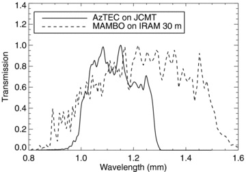
Transmission curves for the AzTEC and MAMBO detectors on their respective telescopes.
The combined 1.16 mm map has two significant advantages over the individual 1.1 and 1.2 mm maps: (1) reduced noise (by roughly  ); and (2) increased reliability of secure detections. The AzTEC and MAMBO catalogues include some spurious detections (Perera et al. 2008; Greve et al. 2008); by combining the two (independent) maps, the secure detections in the resulting map may be more reliable (this is the expectation).
The penalties to pay for these advantages are that the FWHM of the PSF, and the effective wavelength, vary slightly across the 1.16 mm map. Alternatively, we could smooth the two individual raw maps to the same PSF resolution, at the expense of decreased S/N in each pixel. As the weights (defined as wA/σ2A and wM/σ2M) change from pixel to pixel, we average different proportions of AzTEC 1.1 mm and MAMBO 1.2 mm flux densities. Fig. 2 shows the distributions of normalized weights (defined in the legend) from equation (1) for pixels with 1σ < 1 mJy in the combined 1.16 mm map. The majority of pixels in the combined map are in a small range of normalized weights (∼ 0.4 for the AzTEC map, ∼0.6 for the MAMBO map); the variation in FWHM and effective wavelength is small. The central wavelength of the combined map is calculated using these normalized weights and the quoted wavelengths of the two individual maps. The distribution of stacked flux densities for randomly chosen pixels in the combined map has zero mean, as expected based on the individual maps (Section 3).
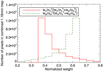
Distribution of normalized weights (equation 1) for pixels with 1σ < 1 mJy in the combined 1.16 mm map. The normalized weights applied to the AzTEC and MAMBO maps for each pixel sum to 1, so the histograms are symmetric about 0.5.
The area in our combined 1.16 mm map with 1σ < 1 mJy is 0.082 deg2. We use the overlap between this region and the area covered by the 24 μm sources (0.068 deg2) for the stacking analysis. While we focus on stacking using the combined 1.16 mm map due to its uniform depth (reaching 1σ∼ 0.5 mJy), we also compare the stacking results using the SCUBA 850 μm survey of the GOODS-N region. The cleaned (of secure detections) 850 μm map (Pope et al. 2005) has a non-uniform, non-contiguous 0.031 deg2 area with 0.5 < 1σ < 5 mJy. We ensure that both the clean and full SCUBA maps have a mean flux density of 0 mJy in the area with 24 μm sources.
Our terminology is as follows: map refers to a map convolved with its PSF, except when prefaced with ‘raw’; secure detections are directly detected sources in the mm map – that is, non-spurious sources in the AzTEC 1.1 mm and MAMBO 1.2 mm maps, and sources with S/N ≥ 3.8 in the combined 1.16 mm map (see Section 2.2 for a justification of this threshold); hereafter, when we use the word sources we mean sources in an external catalogue that are not detected in the mm maps. A cleaned map has all secure detections subtracted before convolution with the PSF (Section 3.2), whereas a full map contains the secure detections.
The combined 1.16 mm map is publicly available at http://www.astro.umass.edu/~pope/goodsn_mm/.
2.2 Verifying the 1.16 mm map
Detections in the combined 1.16 mm map are found by searching for peaks in the S/N map. As the S/N threshold is decreased, there is an increasing probability that some detections are spurious. Perera et al. (2008) and Greve et al. (2008) determine which detections, in their AzTEC 1.1 mm and MAMBO 1.2 mm maps, are most likely spurious; most spurious detections have S/N (before deboosting) <3.8, and only five secure detections have S/N (before deboosting) <3.8. We use this S/N threshold to make our secure detection list for the combined map. Positions and measured flux densities of secure 1.16 mm detections are given in Table 1.
Secure detections in the combined 1.16 mm map (a weighted average of AzTEC 1.1 mm and MAMBO 1.2 mm maps).
| Number | RA | Dec. | Smeasured (mJy) | σ (mJy) | S/N | Sdeboosted (mJy) | AzTEC ID | MAMBO ID |
| 1 | 189.299114 | 62.369436 | 10.26 | 0.68 | 15.0 | … | AzGN01 | GN1200.1 |
| 2 | 189.137896 | 62.235510 | 5.24 | 0.57 | 9.1 | 5.2 | AzGN03 | GN1200.2 |
| 3 | 189.378717 | 62.216051 | 4.51 | 0.55 | 8.2 | 4.4 | AzGN05 | GN1200.4 |
| 4 | 189.297686 | 62.224436 | 4.09 | 0.54 | 7.6 | 3.9 | AzGN07 | GN1200.3 |
| 5 | 189.132927 | 62.286617 | 4.22 | 0.56 | 7.5 | 4.1 | AzGN02 | GN1200.13 |
| 6 | 189.112273 | 62.101043 | 4.81 | 0.67 | 7.2 | 4.5 | AzGN06 | GN1200.5 |
| 7 | 188.959560 | 62.178029 | 5.00 | 0.71 | 7.0 | 4.6 | AzGN04 | GN1200.12 |
| 8 | 189.308576 | 62.307210 | 3.46 | 0.57 | 6.1 | 3.1 | AzGN26 | GN1200.6 |
| 9 | 189.149018 | 62.119408 | 3.35 | 0.61 | 5.5 | 2.9 | AzGN11 | GN1200.14 |
| 10 | 189.190353 | 62.244432 | 3.02 | 0.56 | 5.4 | 2.6 | AzGN08 | … |
| 11 | 188.973386 | 62.228058 | 3.10 | 0.60 | 5.1 | 2.6 | AzGN13 | GN1200.15 |
| 12 | 189.184207 | 62.327207 | 3.03 | 0.59 | 5.1 | 2.5 | AzGN28 | GN1200.9 |
| 13 | 189.138377 | 62.105511 | 3.31 | 0.66 | 5.0 | 2.7 | AzGN12 | … |
| 14 | 189.213067 | 62.204995 | 2.88 | 0.57 | 5.0 | 2.4 | AzGN14 | GN1200.25 |
| 15 | 189.501924 | 62.269772 | 3.26 | 0.66 | 4.9 | 2.7 | AzGN21 | … |
| 16 | 189.202112 | 62.351658 | 3.05 | 0.63 | 4.8 | 2.5 | … | … |
| 17 | 189.214098 | 62.339995 | 2.88 | 0.60 | 4.8 | 2.3 | … | … |
| 18 | 189.068612 | 62.254326 | 2.61 | 0.55 | 4.7 | 2.1 | AzGN16 | … |
| 19 | 189.300036 | 62.203880 | 2.59 | 0.55 | 4.7 | 2.1 | … | GN1200.29 |
| 20 | 189.114187 | 62.203822 | 2.61 | 0.57 | 4.6 | 2.1 | AzGN10 | … |
| 21 | 189.407721 | 62.292688 | 2.62 | 0.58 | 4.5 | 2.1 | AzGN09 | … |
| 22 | 189.400013 | 62.184363 | 2.63 | 0.58 | 4.5 | 2.1 | … | GN1200.17 |
| 23 | 189.440268 | 62.148758 | 3.84 | 0.85 | 4.5 | 2.8 | … | … |
| 24 | 189.035270 | 62.244279 | 2.46 | 0.56 | 4.4 | 1.9 | AzGN24 | … |
| 25 | 189.575648 | 62.241841 | 3.56 | 0.82 | 4.3 | 2.6 | … | … |
| 26 | 188.951634 | 62.257458 | 2.84 | 0.66 | 4.3 | 2.1 | AzGN15 | … |
| 27 | 189.421566 | 62.206005 | 2.41 | 0.57 | 4.3 | 1.9 | AzGN18 | … |
| 28 | 188.942743 | 62.192993 | 3.09 | 0.73 | 4.3 | 2.3 | … | … |
| 29 | 189.216774 | 62.083885 | 3.74 | 0.88 | 4.2 | 2.6 | AzGN25 | … |
| 30 | 188.920762 | 62.242944 | 3.01 | 0.71 | 4.2 | 2.2 | AzGN17 | … |
| 31 | 189.323691 | 62.133314 | 2.74 | 0.67 | 4.1 | 2.0 | … | GN1200.23 |
| 32 | 189.033574 | 62.148164 | 2.42 | 0.60 | 4.0 | 1.8 | … | GN1200.7 |
| 33 | 189.090016 | 62.268797 | 2.23 | 0.56 | 4.0 | 1.7 | … | … |
| 34 | 189.143551 | 62.322737 | 2.44 | 0.61 | 4.0 | 1.8 | … | … |
| 35 | 189.258342 | 62.214444 | 2.19 | 0.55 | 4.0 | 1.6 | … | … |
| 36 | 189.039961 | 62.255953 | 2.21 | 0.56 | 4.0 | 1.6 | … | … |
| 37 | 188.916328 | 62.212377 | 2.97 | 0.75 | 4.0 | 2.1 | … | … |
| 38 | 189.327507 | 62.231090 | 2.12 | 0.54 | 3.9 | 1.6 | … | … |
| 39 | 189.020746 | 62.114810 | 2.71 | 0.70 | 3.9 | 1.9 | AzGN19 | … |
| 40 | 189.238057 | 62.279444 | 2.14 | 0.56 | 3.8 | 1.5 | … | … |
| 41 | 189.550659 | 62.248008 | 2.78 | 0.73 | 3.8 | 1.9 | … | … |
Columns: RA and Dec. are in decimal degrees, and are reported from the centre of the pixel with maximum S/N (Smeasured/σ). Smeasured and σ are the measured flux density and noise in the 1.16 mm map, and Sdeboosted is the deboosted flux density calculated with equation (3). The AzTEC ID is from Perera et al. (2008), the MAMBO ID is from Greve et al. (2008).
Flux boosting is an important issue for detections at low S/N thresholds, particularly when the differential counts distribution (dN/dS) is steep, so that it is more likely for a faint detection's flux density to scatter up than for a bright detection's flux density to scatter down. Flux deboosting is a statistical correction to the measured flux density of a secure detection (Hogg & Turner 1998). The deboosting correction relies on a simulated map using a model of the differential counts distribution (see Coppin et al. 2005). A simulation of the 1.16 mm map is subject to large uncertainties because we do not have exact knowledge of the PSF, so we choose to deboost the flux densities of secure detections using an empirical approach.
Fig. 3 shows the comparison between deboosted flux densities for secure 1.16 and 1.1 mm detections. The combined 1.16 mm map recovers the majority of secure detections identified in the AzTEC 1.1 mm map – the arrows pointing down show that there are four secure detections in the AzTEC map that are not secure detections in the combined map.
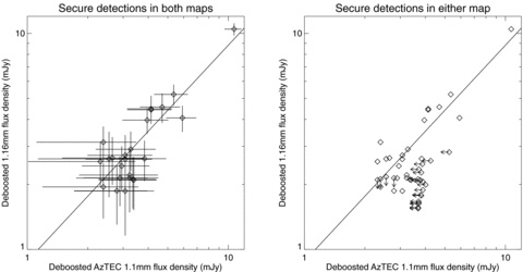
Left-hand panel: empirically deboosted combined 1.16 mm flux density (Sdeboosted) as a function of deboosted AzTEC 1.1 mm flux density (SA,deboosted) for detections which are secure in both maps. The solid line is the best-fitting line to the deboosted flux densities of secure detections (Sdeboosted = 0.88SA,deboosted). Right-hand panel: a comparison of deboosted flux densities for secure detections in either map. If a secure 1.16 mm detection does not coincide with a secure AzTEC 1.1 mm detection, a 3.8σ upper limit on the AzTEC 1.1 mm flux density is plotted. Similarly, if a secure AzTEC 1.1 mm detection does not coincide with a secure 1.16 mm detection, a 3.8σ upper limit on the 1.16 mm flux density is plotted.
Fig. 4 shows the comparison between deboosted flux densities for secure 1.16 and 1.2 mm detections. There are 14 secure detections in the MAMBO 1.2 mm map that are not coincident with secure detections in the combined 1.16 mm map (the down arrows in the right-hand panel). However, the upper limits to the flux densities in the combined map are within the scatter about the solid line.
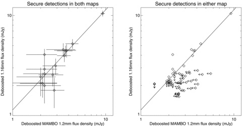
Left-hand panel: empirically deboosted combined 1.16 mm flux density (Sdeboosted) as a function of deboosted MAMBO 1.2 mm flux density (SM,deboosted) for detections which are secure in both maps. The solid line is the best-fitting line to the deboosted flux densities of secure detections (Sdeboosted = 1.14SM,deboosted). Right-hand panel: a comparison of deboosted flux densities for secure detections in either map. If a secure 1.16 mm detection does not coincide with a secure MAMBO 1.2 mm detection, a 3.8σ upper limit on the MAMBO 1.2 mm flux density is plotted. Similarly, if a secure MAMBO 1.2 mm detection does not coincide with a secure 1.16 mm detection, a 3.8σ upper limit on the 1.16 mm flux density is plotted. Based on this figure and Fig. 3, we conclude that our method of combining the AzTEC 1.1 mm and MAMBO 1.2 mm maps is valid.
We conclude, based on the comparisons in Figs 3 and 4, that our method of combining the AzTEC 1.1 mm and MAMBO 1.2 mm maps is effective. The combined 1.16 mm map has 13 new secure detections (Table 1); we do not expect the new detections to be in the individual maps.
2.3 GOODS-N MIPS 24 μm redshift catalogue
Galaxies with detected 24 μm emission compose the most homogeneous set of dusty galaxies whose mm flux density can be stacked with significant results. We use the 24 μm catalogue from the GOODS-N Spitzer/MIPS survey, which has a uniform depth of 1σ∼ 5 μJy in the regions of interest (Chary et al. in preparation); the 24 μm fluxes are measured at the positions of IRAC sources, so this catalogue pushes to faint 24 μm fluxes. We only stack ≥3σ 24 μm sources with S24 > 25 μJy. At flux densities above 50 μJy, the catalogue is 99 per cent complete; for 25 < S24 < 50 μJy, the catalogue is 83 per cent complete (Magnelli et al. 2009). Completeness corrections to our results are negligible, so we do not apply them. We exclude sources that lie in the region of the 1.16 mm map with 1σ > 1 mJy; in this region, the noise is non-uniform. The final 24 μm catalogue for stacking has 2484 sources in 0.068 deg2.
To decompose the contribution to the mm background from 24 μm sources as a function of redshift, we require either a photometric or spectroscopic redshift for each 24 μm source. We start by matching a source with a spectroscopic redshift from the catalogues of Barger, Cowie & Wang (2008) and Stern et al. (in preparation) to each 24 μm source. The match radius, 0.7 arcsec, is chosen by maximizing the number of unique matches while minimizing the number of multiple matches. We find spectroscopic redshifts for 1026 (41 per cent of the) 24 μm sources.
If no (or multiple) coincident sources with spectroscopic redshifts are found, we resort to the photometric redshift source catalogue of Brodwin et al. (in preparation) to find a source match. Photometric redshifts are constrained with deep UBVRIzJK imaging, and provide redshift estimates for 872, or 35 per cent, of the 24 μm sources. Photometric redshift uncertainties are small compared to our redshift bins, since we are interested in the contribution to the background from galaxies in large redshift bins. If no (or multiple) coincident sources with photometric redshifts are found, we assign the 24 μm source to a ‘redshift unknown’ bin in the stacking analysis. Of the 2484 24 μm sources, 588 (24 per cent) have no spectroscopic or photometric redshift estimate available.
3 STACKING ANALYSIS
Our stacking procedure depends on two fundamental properties of the (sub)mm maps.
Every detection, and source, is a point source. The PSFs are large; in all three maps the full-width-half-maxima (FWHM) are >10 arcsec. This property has a number of implications. To make low S/N detection-finding easier, the raw maps are convolved with their PSFs; the result is a map where each pixel value is the flux density of a point source at the position of the pixel. Thus, to stack the millimetre flux densities of sources, we require only the values of single pixels in the map.
The means of the maps are 0 mJy. These millimetre observations are taken, filtered and reduced in such a way that the sum of all pixel values in the map is zero. In other words, the most likely value of a randomly chosen pixel is 0 mJy, a useful statistical property we explore in Section 3.1. However, the large PSF forces us to carefully consider the effects of having multiple sources clustered in the area covered by one PSF (also in Section 3.1).
Stacking is the process of averaging the flux density, at some wavelength (1.16 mm), of sources detected at another wavelength. To resolve the (sub)mm background, we want to stack a catalogue of sources whose emission correlates strongly with 1.16 mm emission, and we want this catalogue to have a large number of sources. A catalogue that meets these requirements has galaxies selected on dust emission at both low and high redshift. We do not expect a sample of stellar mass selected sources (e.g. at 3.6 μm) to be efficient at isolating the galaxies responsible for the mm background, because 3.6 μm sources are a mix of dusty and non-dusty galaxies. The MIPS catalogue of 24 μm sources, though, is selected on dust emission to high redshift, and there is a known correlation between the flux densities at mid-infrared and far-infrared wavelengths (Chary & Elbaz 2001).
3.1 The effects of angular clustering on stacking analyses
The undetected mm emission from a 24 μm source covers the area of the mm PSF, so a natural question to ask is: ‘what happens to the stacked mm flux density when there are multiple 24 μm sources in the area encompassed by one mm PSF?’ We revisit the fundamental properties of the mm maps to answer this question.
Consider a randomly distributed population of sources. We are interested in the best estimate of the mm flux density of source A, a source with many neighbours. We remember that 0 mJy is the most likely flux density of a randomly chosen pixel; an equivalent statement is that the total flux at the position of A from all of As randomly distributed neighbours is 0 mJy. To rephrase qualitatively, there are a few neighbours with angular separations small enough to contribute positive flux density at the position of A, but there are many more neighbours with angular separations that are large enough to contribute negative flux density at the position of A. If we have randomly distributed sources in the area covered by the mm PSF, the true flux densities of the sources are the measured flux densities in the mm map. Marsden et al. (2009) prove that in the case of randomly distributed sources, stacking is a measure of the covariance between the stacked catalogue and the (sub)mm map.
Let us also consider a population of sources that is not randomly distributed – a population that is angularly clustered (as we expect the 24 μm sources to be). If the clustering is significant at angular separations where the PSF is positive, and if it is negligible at larger angular separations, the positive contribution at the position of A from the many sources that have small angular separations is not cancelled out by the negative contribution from the sources that have large angular separations. In this case, the measured flux density of A is higher than the true flux density – and thus, we cannot blindly stack multiple sources in the same PSF area. The stacked flux density of angularly clustered sources near secure detections is overestimated for the same reason. The ratio of the measured flux densities to the true flux densities for an ensemble of sources is a function of the angular clustering strength of the sources, the flux densities at the wavelength we stack at and the size of the PSF. We detail our simulation to compute this ratio for the 24 μm sources and the (sub)mm PSF in Section 3.2. We further consider the angular clustering of sources with secure (sub)mm detections; the tests we perform suggest that this angular clustering is the dominant source of overestimating the stacked flux density.
The aim of the next section is to investigate the impact of angular clustering on the stacked (sub)mm flux densities of 24 μm sources. Using a similar analysis, Chary & Pope (2010) conclude that clustering leads to a significant overestimate of the flux density when stacking on BLAST (sub)mm maps with larger PSFs than those for the SCUBA 850 μm and 1.16 mm maps.
The angular clustering of 24 μm sources is uncertain, though spatial clustering measurements exist (Gilli et al. 2007). The assumption we test is that this spatial (three-dimensional) clustering projects to an angular (two dimensional) clustering, which may lead to an overestimate of the stacked flux density.
3.2 Quantifying the effects of angular clustering
The two tests of our assertion of angular clustering are as follows.
An estimate of the ratio of measured flux densities to true flux densities for a simulated map composed solely of 24 μm sources. This test quantifies the effect of angular clustering of 24 μm sources in the area of one PSF. Here, true flux density is an input flux density, and measured flux density is an output flux density (after the simulation).
A comparison of the resolved background from stacking on a cleaned map with the resolved background from stacking on a full map. This test helps address the effect of angular clustering of 24 μm sources with secure (sub)mm detections.
Both tests require a well-characterized PSF: for the first, in order to create a realistic simulated map, and for the second, in order to subtract the secure (sub)mm detections to create a clean map. The 1.16 mm map does not have a well-characterized PSF, so we perform the tests for the Perera et al. (2008) AzTEC 1.1 mm map, with an area defined by 1σ < 1 mJy (0.070 deg2). We also run the tests for the SCUBA 850 μm map, with an area defined by 1σ < 5 mJy (0.031 deg2).
3.2.1 The first test
Our first test is a simulation of an AzTEC 1.1 mm map composed exclusively of 24 μm sources. Using the relation between 24 μm flux density and stacked 1.1 mm flux density (the differential form of Fig. 7), we insert best estimates of the 1.1 mm flux densities at the positions of all the 24 μm sources. This process preserves the angular clustering of the real 24 μm sources. We then convolve the simulated map with the AzTEC PSF, and remeasure the 1.1 mm flux densities (by stacking). The stacked flux density, multiplied by the number of sources, is the measured flux density of the entire sample, while the true flux density is the sum of the inserted flux densities. The ratio of total measured flux density to total true flux density is ∼1.08. Due to angular clustering of multiple sources within the average PSF, the stacked 1.1 mm flux density of 24 μm sources appears to be overestimated by ∼8 per cent. Different relations between 24 μm flux density and 1.1 mm flux density that are physically motivated (e.g. from Chary & Elbaz 2001) produce comparable ratios. This 8 per cent correction to the stacked 1.1 mm flux density is within the uncertainties (e.g. from the relation between 24 μm and 1.1 mm flux densities).
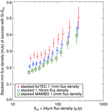
Stacked AzTEC 1.1 mm, combined 1.16 mm and MAMBO 1.2 mm flux densities from 24 μm sources with flux densities > S24. The stacked 1.1 mm flux densities are higher than the stacked 1.2 mm flux densities, as expected for the SED of a typical dusty galaxy. The 1.16 mm flux density lies between and has smaller errors than the 1.1 and 1.2 mm flux densities.
An alternative test to the one just presented is an extension of the deblending method in Greve et al. (2010) and Kurczynski & Gawiser (2010). Deblending is the simultaneous solution of a system of Q equations that are mathematical descriptions of the flux densities of blended, angularly clustered sources (Q is the number of sources to be stacked, see Section 5.2 and fig. 5 in Greve et al. 2010). The result of deblending is a vector of the true source flux densities. Our extension of the methods in Greve et al. (2010) and Kurczynski & Gawiser (2010) generalizes the equations by not assuming a Gaussian PSF – which does not have the negative parts that are important for the data we consider here – but instead uses the AzTEC PSF for deblending the sources in the AzTEC map. Our extension does not account for 24 μm undetected sources that may affect the stacked 1.1 mm flux of 24 μm sources. This deblending procedure gives the same answer as our simulations: an 8 per cent overestimation of the stacked 1.1 mm flux density.
3.2.2 The second test
Our procedure for cleaning the raw AzTEC 1.1 mm map is: (1) for each secure 1.1 mm detection, scale the PSF to the deboosted flux density; (2) subtract the scaled PSFs from the raw map and (3) convolve the residual map with the PSF. There are two components to the resolved 1.1 mm background: the contribution to the background from stacking 24 μm sources, and the contribution to the background from the secure 1.1 mm detections cleaned from the map. The latter is calculated by summing the deboosted flux densities of all the secure detections and dividing by the area.
We compare the 1.1 mm background resolved from stacking on the full and cleaned maps in Fig. 5 (values in Table 2). A stack of 24 μm sources on the full map, when compared to a stack on the cleaned map, does not significantly overestimate the resolved 1.1 mm background.
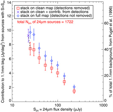
The resolved 1.1 mm background from 24 μm sources with flux densities > S24. The red squares are a stack on the cleaned map; the blue triangles are a stack on the full map. The purple ‘X’ includes the contribution to the background from the secure 1.1 mm detections, arbitrarily added to the faintest cumulative flux density bin, after stacking on the cleaned map. Angular clustering of 24 μm sources with secure 1.1 mm detections does not appear to cause a significant overestimate of the resolved 1.1 mm background.
A comparison of the resolved background at 850 μm and 1.1 mm using SCUBA and AzTEC maps (full and cleaned).
| Map | 850 μm bkg (Jy deg−2) | 1.1 mm bkg (Jy deg−2) |
| Full | 27.0 ± 1.6 | 9.7 ± 0.9 |
| Cleaned | 12.5 ± 1.6 | 7.4 ± 0.9 |
| Cleaned + detections | 21.1 ± 1.7 | 9.2 ± 0.9 |
| Map | 850 μm bkg (Jy deg−2) | 1.1 mm bkg (Jy deg−2) |
| Full | 27.0 ± 1.6 | 9.7 ± 0.9 |
| Cleaned | 12.5 ± 1.6 | 7.4 ± 0.9 |
| Cleaned + detections | 21.1 ± 1.7 | 9.2 ± 0.9 |
Fig. 5 implies the clustering of 24 μm sources with the secure detections in the 1.16 mm map will have a small effect on the stacked flux density, although we note that the combined 1.16 mm map does have more secure detections (in a larger area with 1σ < 1 mJy) than the AzTEC 1.1 mm map.
The cleaned 850 μm map is from Pope et al. (2005). We compare the 850 μm background resolved from stacking on the full and cleaned maps in Fig. 6. The blue diamonds (values in Table 2) show that a stack of 24 μm sources on the full 850 μm map overestimates the resolved sub-mm background, when compared to a stack on the cleaned map. We hesitate to attribute the entire difference to angular clustering of 24 μm sources with the secure 850 μm detections; the difference is probably due to many effects.
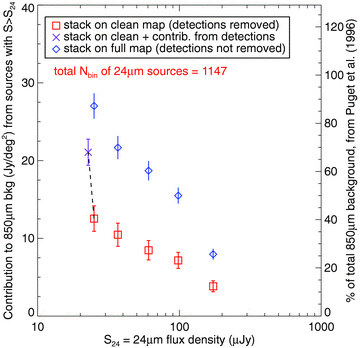
The resolved 850 μm background from 24 μm sources with flux densities > S24. The red squares are a stack on the cleaned map; the blue diamonds are a stack on the full map. The purple ‘X’ includes the contribution to the background from the secure 850 μm detections, arbitrarily added to the faintest cumulative flux density bin, after stacking on the cleaned map. In reality, the 24 μm counterparts to the secure 850 μm detections have flux densities ranging from S24∼ 20–700 μJy (Pope et al. 2006). We adopt the background values from stacking on the cleaned map.
Over-subtraction of the secure 850 μm detections in making the cleaned map. Detections are subtracted using measured, rather than deboosted, flux densities. To estimate the magnitude of this over-subtraction we clean the raw AzTEC 1.1 mm map using both measured and deboosted flux densities for the secure 1.1 mm detections, and find a marginal difference in the resolved 1.1 mm background between the two methods. The average deboosting correction – roughly 30 per cent of the measured flux subtracted off (Perera et al. 2008; Pope et al. 2006) – is similar for both the 850 μm and 1.1 mm detections; combined with the marginal difference in resolved 1.1 mm background, these suggest that the resolved 850 μm background is insensitive to the over-subtraction of the secure 850 μm detections in the cleaned map.
Over-subtraction of the secure 850 μm detections in regions of the map close to the confusion limit. The measured and deboosted flux densities of the detections in the deepest parts of the 850 μm map are not corrected for the contribution from blended sources below the detection limit. We compare the background resolved from stacking on the full and cleaned maps again, this time excluding regions around all detections with 1σ < 1 mJy; a large difference in the resolved background remains.
Non-uniform noise, which complicates interpretation of the results from the inverse-variance weighted stacking formula.
Different chop throws across the SCUBA map, which complicates the angular separations where we expect to see negative emission from detections.
Angular clustering of the 24 μm sources with the secure 850 μm detections.
A simulation of the 850 μm map, similar to our first test except using randomly distributed sources drawn from a differential counts distribution (dN/dS) and an idealized SCUBA PSF, implies that part of the difference may be due to effects other than angular clustering (e.g. effects 1–4). If this simulation is correct, the stacked 850 μm flux density is underestimated when using the cleaned map, and our estimate of the resolved 850 μm background is a lower limit. However, the ratio of stacked 850 μm to 1.16 mm flux density as a function of redshift (using the full 850 μm map) requires a model SED with a higher temperature than 60 K (assuming an emissivity index β of 1.5). We therefore use the 850 μm flux density from stacking on the cleaned map. With large, uniform maps from SCUBA-2 these issues can be tested and resolved – until we have such maps, we cannot separate the effects of angular clustering and non-uniform noise.
In conclusion, we find the following.
In the specific case of the 24 μm sources and the 1.16 mm map and its PSF, the effects due to angular clustering are additional corrections within the statistical uncertainty of the stacked flux density.
We cannot separate the effect of angular clustering from the effect of non-uniform noise in the SCUBA 850 μm map.
The results we present in Section 4 use the cleaned 850 μm map (with the contribution from the secure 850 μm detections added after stacking) and the full 1.16 mm map.
4 RESULTS AND DISCUSSION
The stacked 1.16 mm flux density as a function of cumulative 24 μm source flux density is shown in Fig. 7. This provides another validation of our method of combining the AzTEC 1.1 mm and MAMBO 1.2 mm maps; the combined 1.16 mm map values (blue diamonds) lie between the stacked flux densities for the individual maps. The stack on the combined 1.16 mm map has smaller errors than the stacks on the individual maps, as anticipated from equation (2).
We multiply the stacked flux density (Fig. 7) by the number of 24 μm sources in the cumulative bin and divide by the area to get the contribution to the background (Fig. 8). The overlap between the 1.16 mm map area with 1σ < 1 mJy and the 24 μm exposure map defines A (0.068 deg2). The blue diamonds show that 24 μm sources resolve 7.6 ± 0.4 Jy deg−2 of the 1.16 mm background.
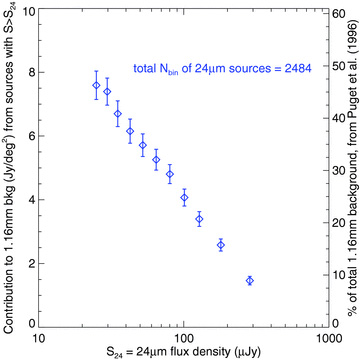
Contribution to the 1.16 mm background from 24 μm sources with flux densities > S24.
The total CIB at (sub)mm wavelengths is uncertain due to large-scale variability of cirrus emission in the Galaxy that must be subtracted from the observed background, which is measured using COBE maps. At 1.16 mm, the published estimates for the total background are 16.4 Jy deg−2 (Puget et al. 1996) and 22.0 Jy deg−2 (Fixsen et al. 1998) (Table 3).
The total background at four wavelengths.
| Wavelength (mm) | Puget et al. (1996) (Jy deg−2) | Fixsen et al. (1998) (Jy deg−2) | Adopted (Jy deg−2) |
| 0.85 | 31 | 44+5−8 | 40 ± 9 |
| 1.1 | 18.3 | 24.8+1.7−4.0 | … |
| 1.16 | 16.4 | 22.0+1.4−3.4 | 19.9 ± 3.5 |
| 1.2 | 15.4 | 20.4+1.1−3.0 | … |
| Wavelength (mm) | Puget et al. (1996) (Jy deg−2) | Fixsen et al. (1998) (Jy deg−2) | Adopted (Jy deg−2) |
| 0.85 | 31 | 44+5−8 | 40 ± 9 |
| 1.1 | 18.3 | 24.8+1.7−4.0 | … |
| 1.16 | 16.4 | 22.0+1.4−3.4 | 19.9 ± 3.5 |
| 1.2 | 15.4 | 20.4+1.1−3.0 | … |
The left-hand panel in Fig. 9 shows the resolved 1.16 mm background decomposed into redshift bins. Photometric redshift errors for individual 24 μm sources should be negligible in bins of this size. The highest redshift bin is for all sources with z > 1.33, but we plot it out to z = 3 for clarity. We assume that any 24 μm sources that fail to match to unique sources with redshift estimates (either spectroscopic or photometric) lie at z > 1.3, and we add their contribution to the highest redshift bin.
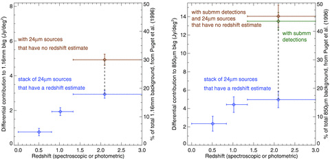
Left-hand panel: the (differential) redshift distribution of the resolved 1.16 mm background from 24 μm sources. The diamonds are plotted at the average redshifts of the bins. The brown diamond contains the contributions from the 24 μm sources with z > 1.3 and the 24 μm sources without a redshift estimate. Right-hand panel: the (differential) redshift distribution of the resolved 850 μm background from 24 μm sources. We use the same redshift bins as in the left-hand panel. The y-axes in both panels show the levels at which the backgrounds are 50 per cent resolved. Most of the resolved background at the two wavelengths comes from galaxies at z > 1.3.
The 1.16 mm background is not fully resolved by 24 μm sources with S24 > 25 μJy; most of the portion that is resolved comes from galaxies at high redshift (z > 1.3). We repeat our stacking analysis on the cleaned 850 μm map to investigate the differences in the resolved portions of the background at 850 μm and 1.16 mm.
We use the same redshift bins as in the 1.16 mm analysis (the right-hand panel in Fig. 9). At 850 μm, the values for the total background are 31 Jy deg−2 (Puget et al. 1996) and 44 Jy deg−2 (Fixsen et al. 1998) (Table 3). The contribution from the secure 850 μm detections is added to the contribution derived from stacking the 24 μm sources on the cleaned map; all secure 850 μm detections have 24 μm counterparts, and we assume for simplicity that the detections lie at z > 1.3. This assumption is reasonable, since only four of the 33 detections appear to lie at z < 1.3 (Pope et al. 2006), and these four account for <5 per cent of the contribution from the detections.
Our analysis does not definitively provide the redshift origins of the total 850 μm background, since it is not completely resolved by 24 μm sources. The results suggest that a large fraction of the resolved 850 μm background originates in galaxies at z > 1.3. Wang et al. (2006) perform a stacking analysis and conclude that more than half of the background at 850 μm comes from galaxies at low redshifts (z < 1.5). Our methodology differs from that of Wang et al. (2006): they stack a near infrared (H+3.6 μm) sample on a full map with the 850 μm detections.
We show that the background at 850 μm and 1.16 mm is only partially resolved. Can we provide any constraints on the redshifts of the galaxies that contribute to the remainder of the 1.16 mm background?
There are two often used estimates for the total background at these two wavelengths. We adopt the average of the range allowed by the two estimates: 19.9 ± 3.5 Jy deg−2 at 1.16 mm, and 40 ± 9 Jy deg−2 at 850 μm (Table 3). If we assume that the galaxies responsible for the remaining unresolved 850 μm background are distributed to maintain the redshift distribution of the galaxies contributing to the resolved background, then the final decomposition of the 850 μm background is [z∼ 0.4, z∼ 1, z > 1.3]=[4.5 ± 1.6 Jy deg−2, 8.5 ± 1.6 Jy deg−2, 27 ± 2 Jy deg−2]. The errors maintain the S/N of the redshift bins of the resolved background. We also assume that the ratios of the resolved 850 μm to 1.16 mm background as a function of redshift (last column of Table 4) hold for the total 850 μm background; we thus convert each contribution to the 850 μm background into an estimate of the contribution to the 1.16 mm background. The decomposition of the 1.16 mm background is thus 4.5/3.1 + 8.5/2.3 + 27/2.9 = 14.4 ± 0.85 Jy deg−2. The rest of the 1.16 mm background, which is 19.9–14.4 = 5.4 ± 0.85 Jy deg−2, presumably comes from galaxies at z > 1.3, where the observed submm to mm flux density ratio is lower than the values we use (see e.g. fig. 13 in Greve et al. 2004). The sum of all contributions from galaxies at z > 1.3 is 14.8 ± 1.1 Jy deg−2, or 74 ± 14 per cent of the total 1.16 mm background. This likely scenario for the unresolved background is shown with filled bars in Fig. 10.
The redshift distribution of the resolved background at 1.16 mm and 850 μm from 24 μm sources.
| z | Sbin,1.16 (mJy) | Nbin,1.16 | per cent w/spec-z | 1.16 mm bkg (Jy deg−2) | Sbin,850 (mJy) | Nbin,850 | 850 μm bkg (Jy deg−2) | 850/1.16 |
| 0–0.82 | 0.090 ± 0.025 | 576 | 75 | 0.76 ± 0.21 | 0.237 ± 0.081 | 304 | 2.34 ± 0.81 | 3.1 ± 1.4 |
| 0.82–1.33 | 0.199 ± 0.023 | 660 | 64 | 1.94 ± 0.23 | 0.402 ± 0.077 | 338 | 4.42 ± 0.85 | 2.3 ± 0.5 |
| >1.33 | 0.302 ± 0.023 | 660 | 26 | 2.94 ± 0.23 | 0.492 ± 0.087 | 310 | 4.97 ± 0.88 | 1.7 ± 0.3 |
| With 850 μm detections added to highest z bin | ||||||||
| >1.33 | … | 660 | … | 2.94 ± 0.23 | … | 343 | 13.50 ± 0.95 | 4.6 ± 0.5 |
| With ‘redshift unknown’ added to highest z bin | ||||||||
| >1.33 | … | 1248 | … | 4.92 ± 0.32 | … | 538 | 14.04 ± 1.23 | 2.9 ± 0.3 |
Columns: Sbin,1.16 is the stacked 1.16 mm flux density of Nbin,1.16 sources; Sbin,850 is the stacked 850 μm flux density of Nbin,850 sources. Column 4 is the percentage of the Nbin,1.16 sources that have a redshift determined spectroscopically. Columns 5 and 8 are the resolved background in each bin. Column 9 is the resolved 850 μm background divided by the resolved 1.16 mm background.
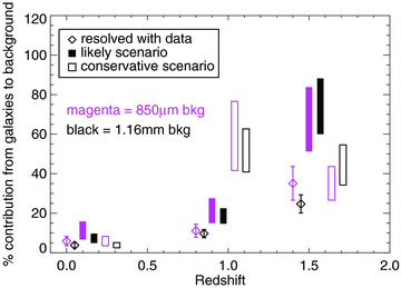
The redshift origins of the background at 850 μm and 1.16 mm under various scenarios (see Section 4 for details). The different plotting styles indicate different scenarios; all magenta points/bars are for the 850 μm background, while all black points/bars are for the 1.16 mm background. Points/bars are offset within the redshift bins for clarity. In what we deem the most likely scenario, 60–88 per cent of the 1.16 mm background comes from galaxies at z > 1.3.
Although we cannot quantify the probability that the unresolved 850 μm background is distributed as the resolved background, we are able to derive a lower limit to the amount of the total 1.16 mm background that comes from galaxies at z > 1.3. In a conservative scenario, all of the remaining unresolved 850 μm background comes from galaxies at z < 1.3. Assuming the ratio of 2.3 at z∼ 1 holds for the total background, an additional contribution of 40 – 2.3–4.4–14 = 19.3 Jy deg−2 at 850 μm corresponds to an additional contribution of 8.4 Jy deg−2 at 1.16 mm. If the unresolved 850 μm background is produced only by z < 1.3 galaxies, the contribution to the 1.16 mm background is 0.8 + 10.3 + 4.9 = 16 ± 1.3 Jy deg−2. Again, the remaining 19.9 – 16= 3.9 ± 1.3 of the 1.16 mm background comes from galaxies at z > 1.3. At minimum, 44 ± 10 per cent of the total 1.16 mm background comes from galaxies at z > 1.3. This conservative scenario is illustrated with unfilled bars in Fig. 10.
An alternate explanation to both scenarios is that all the unresolved background comes from a population of low-redshift galaxies with very cold dust and no warm dust (i.e. a population of galaxies with a disproportionate amount of large dust grains relative to small dust grains). Our decomposition of the (sub)mm background depends on selecting dusty galaxies at 24 μm– the selection could miss galaxies with little or no warm dust. Galaxies with an excess of cold dust need dust temperatures in the realm of ∼10 K at z∼ 1, and lower temperatures at lower redshifts, to account for the ratio of unresolved 850 μm to 1.1 mm background; large numbers of galaxies are unlikely to have these extreme dust temperatures.
In this paper, we use observational constraints on the fraction of the (sub)mm background that is resolved to hypothesize that 60–88 per cent of the 1.16 mm background comes from high-redshift galaxies. In order to resolve the total 1.16 mm background and provide direct constraints on the redshifts of the galaxies, we need improvements in both the catalogue to be stacked and the mm map. Any stacking catalogue must be deep and homogeneously selected across a large redshift range. The GOODS-N survey at 100 μm with Herschel will reach similar (total infrared luminosity) depths as the deepest surveys at 24 μm with Spitzer; furthermore, the flux density from 100 μm sources should correlate more tightly with mm flux density than does the flux density from 24 μm sources (dust emitting at 100 μm is a better tracer of the dust emitting at 1 mm). Much deeper radio catalogues than currently exist for stacking, using EVLA and ALMA, are also promising. Alternatively, future large dish (sub)mm telescopes, such as the Large Millimetre Telescope, will provide maps in which the bulk of the galaxies that contribute to the cosmic millimetre background are individually detected. Models presented in Chary & Pope (2010) predict that 60 per cent of the 1.2 mm background comes from galaxies with 1.2 mm flux densities higher than 0.06 mJy (30 times deeper than the combined map).
5 CONCLUSIONS
We create a deep (σ∼ 0.5 mJy) 1.16 mm map by averaging the AzTEC 1.1 mm and MAMBO 1.2 mm maps in the GOODS-N region. We verify the properties of this map by examining both the deboosted flux densities of the 41 secure detections and the stacked flux density of 24 μm sources. Of the 41 secure detections, 13 are new.
We test the effects of angular clustering of 24 μm sources on the stacked (sub)mm flux density. While clustering does not seem to lead to a significant overestimate of the stacked 1.16 mm flux density, it may be responsible for part of the overestimate of the stacked 850 μm flux density.
24 μm sources resolve 7.6 Jy deg−2 (31–45 per cent) of the 1.16 mm background; 3 Jy deg−2 comes from galaxies at z > 1.3. 24 μm sources resolve 12.3 Jy deg−2 (23–39 per cent) of the 850 μm background, and the submillimetre detections contribute an additional 16–26 per cent; 14 Jy deg−2 of the 850 μm background comes from galaxies at z > 1.3.
Using the ratio of the resolved 850 μm background to the resolved 1.16 mm background, we propose that 60–88 per cent of the cosmic millimetre background comes from high-redshift (z > 1.3) galaxies. In the most conservative scenario, 34–55 per cent of the 1.16 mm background comes from galaxies at z > 1.3.
We hope to directly detect the majority of the galaxies contributing to the millimetre background with future surveys using large telescopes (e.g. the LMT). Deeper catalogues for stacking, at radio and far-infrared wavelengths, are needed to fully resolve the mm background. Future studies will also need to assess the effects of angular clustering.
We thank the referee for their helpful comments. This work is based on observations made with the Spitzer Space Telescope, which is operated by the Jet Propulsion Laboratory, California Institute of Technology under a contract with NASA. Support for this work was provided by NASA through an award issued by JPL/Caltech. AP acknowledges support provided by NASA through the Spitzer Space Telescope Fellowship Program, through a contract issued by the Jet Propulsion Laboratory, California Institute of Technology under a contract with NASA. The Dark Cosmology Centre is funded by the DNRF. TRG acknowledges support from IDA. Support for MB was provided by the W. M. Keck Foundation. KC acknowledges the UK Science and Technology Facilities Council (STFC) for a fellowship.
REFERENCES
