


Abstract
We describe Monte Carlo models for the dynamical evolution of the massive globular cluster 47 Tuc (NGC 104). The code includes treatments of two-body relaxation, most kinds of three- and four-body interactions involving primordial binaries and those formed dynamically, the Galactic tide, and the internal evolution of both single and binary stars. We arrive at a set of initial parameters for the cluster which, after 12 Gyr of evolution, gives a model with a fairly satisfactory match to surface brightness and density profiles, the velocity dispersion profile, the luminosity function in two fields and the acceleration of pulsars. Our models appear to require a relatively steep initial mass function for stars above about turnoff, with an index of about 2.8 (where the Salpeter mass function has an index of 2.35), and a relatively flat initial mass function (index about 0.4) for the lower main sequence. According to the model, the current mass is estimated at 0.9 million solar masses, of which about 34 per cent consists of remnants. We find that primordial binaries are gradually taking over from mass loss by stellar evolution as the main dynamical driver of the core. Despite the high concentration of the cluster, core collapse will take at least another 20 Gyr.
1 INTRODUCTION
This is one of a series of papers in which we attempt to construct dynamical evolutionary models of old star clusters in the Milky Way. The first in the series concerned the massive, southern cluster ω Centauri (Giersz & Heggie 2003). That study was a pilot project which used a more primitive version of the code than is available now, especially with regard to stellar evolution. Nevertheless, it yielded quantitative theoretical results on mass segregation, which is usually neglected in studies of this cluster because of its very long relaxation time. Our updated code, more or less in its present form, was then tested in application to the old open cluster M67 (Giersz, Heggie & Hurley 2008), by comparison with existing N-body modelling. Then, we returned to the globular clusters, for which N-body modelling is either impossible or very limited. Our model of the nearby cluster M4 (Heggie & Giersz 2008a) showed that this object appears to have passed through core collapse, despite its uncollapsed (King-like) surface brightness profile. Turning next to the rather similar object NGC 6397 (Giersz & Heggie 2009), which does have a profile of the type thought to be typical of a post-collapse cluster, we found that it should be in a similar evolutionary phase to M4, and concluded that the difference between the two clusters was best explained as a result of fluctuations. Detailed N-body modelling (Heggie & Giersz 2009) confirmed that a post-collapse cluster like NGC 6397 should exhibit oscillations, on a time-scale of the order of 108 yr, as a result of which it could sometimes look like M4, and sometimes like NGC 6397. In summary, each time we have looked at a specific globular cluster with our technique, we have discovered something slightly surprising: mass segregation in ω Cen, the postcollapse status of M4 and core oscillations in NGC 6397.
In the present paper we turn our attention to the other famous, massive, southern globular cluster – 47 Tucanae (NGC 104). Like M4 and NGC 6397 there is a wealth of observations, even though it is considerably more distant. It is also much richer, reducing some statistical errors in such data as the surface brightness distribution. It was selected for detailed study during discussion at the programme ‘Formation and Evolution of Globular Clusters’, held at the Kavli Institute for Theoretical Physics, Santa Barbara, California, USA, in 2009 January, just as M4 had been selected at the MODEST-5 meeting (‘Modelling Dense Stellar Systems’) at McMaster University, Hamilton, Canada, in 2004 August. From the point of view of dynamical evolution, it differs from most of our earlier targets because of its long relaxation time (which is a consequence of its much greater mass). This makes it dynamically younger, raising the expectation that it should be easier to model. But the long relaxation time should also imply that its present state is more directly influenced by its initial conditions.
This paper first reviews both the observational data on 47 Tuc and earlier work on its dynamics (Section 2). Then in Section 3, we discuss our techniques, in terms of the simulation of dynamical evolution, the calculation of mock observational data and our search for satisfactory initial conditions. In the following section (Section 4), we present our optimal model, in the sense that, among the models we have studied, it is representative of those that provide the most satisfactory fit to a wide selection of the available observational data. Finally (Section 5), we consider such issues as the plausibility of our initial conditions, how these relate to current ideas on the earlier stages of cluster formation and evolution, and the mechanisms which dominate the dynamical evolution of the cluster at the present day. Section 6 sums up.
2 A REVIEW OF 47 TUC
2.1 Dynamical models
As with all globular star clusters, dynamical models of 47 Tuc fall into two classes (Heggie & Giersz 2008b): static models, such as King models (King 1966), and dynamical evolutionary models, which are the focus of our own contribution. (We exclude here the practice of fitting a template to such data as the surface brightness profile. Though often referred to as King models, and useful as they are for the measurement of such parameters as the core radius (e.g. Calzetti et al. 1993), they have no real dynamical basis.) In this section we survey existing models of these two kinds, though we often have to refer to various kinds of observational data on which we expand in later sections.
Illingworth & Illingworth (1976) fitted a single-mass King model to a composite surface brightness profile constructed from photometric data and star counts. Simple though it is, such a model was also used more recently by Freire et al. (2001) for a study of pulsar accelerations; and by McLaughlin et al. (2006) for the interpretation of the velocity dispersion profile, derived from proper motions and radial velocities. Several investigators have constructed multi-mass generalizations of the King model for 47 Tuc (Da Costa & Freeman 1985; Meylan & Mayor 1986; Mapelli et al. 2004). Meylan (1988, 1989) and Rees (1996) added anisotropy, in the style of Michie (1963).
A number of other, rather different static models have been constructed for 47 Tuc. It was pointed out by Sau Fa & Pedron (2001) that a better fit to the surface brightness profile could be obtained by construction of a model with a slightly different choice of distribution function from that of King. The rotation of 47 Tuc has been the subject of considerable study, but almost all dynamical models ignore it. One exception is the pair of models constructed by Davoust (1986). Finally in this section we mention the non-parametric analysis of Gebhardt et al. (1995), which derives the distribution function from the observational data.
More in line with the aims and methods of this paper are the dynamical evolutionary models of Murphy et al. (1998) and Behler et al. (2003). Though few details are available in these abstracts, the technique is a multi-mass Fokker–Planck code, with a discretized, piecewise power-law mass function and heavy remnants. The models are able to account for the stellar mass function, star counts, the velocity dispersion profile, pulsar accelerations and the radial distribution of neutron stars. The models fit better than a King–Michie model.
2.2 Observational data
Our purpose in this section is to review something of the wealth of observational data which exists for 47 Tuc. Not all of these data are compatible, and one of our aims is to explain where and why we have selected one data set over another.
2.2.1 Surface brightness profile and star counts
In several of the foregoing investigations the spatial distribution of matter in 47 Tuc has been specified in terms of a surface brightness profile, and two major compilations exist (Meylan 1988; Trager, King & Djorgovski 1995). The later of these is largely a superset of the former, though Meylan (1988) includes star count data in J from Da Costa (1982) which are excluded from the later compilation. The two compilations agree quite well; Trager et al. (1995) also provide an analytic fit to their data, and the rms difference between this and the data in Meylan (1988) is 0.28 mag. A large fraction of this is contributed by star counts at large radius, including the aforementioned J data.
Despite this apparently satisfactory state of affairs, some caution must be exercised in the construction of a composite profile from such disparate data. Da Costa himself (his fig. 7) shows that the slope of the density profile from different plates (differing essentially in the range of masses of the counted stars) is different, in a manner consistent with mass segregation. A further complication is the colour gradient exhibited by 47 Tuc (Chun & Freeman 1979), which has been traced to a radial variation in the fraction of light contributed by bright giants (Freeman 1985). One implication of these results is that it is not strictly possible to reconstruct the surface brightness from star counts by a constant shift, as is done in these compilations. Furthermore, beyond about 5 arcmin, the only genuine photometric data in these compilations are the drift scan measures of Gascoigne & Burr (1956), and an inspection of their fig. 1 does not inspire much confidence in the results at these radii. With this consideration in mind, in our modelling we have not relied solely on the surface brightness profile of Trager et al. (1995), but have also compared our models with counts from two sources, (i) the two deepest V data in the compilation of Trager et al. (1995), i.e. plates 3407 and 3754 from Da Costa (1982), and (ii) the surface density profile (based on star counts for stars above turnoff mass in the innermost 82.5 arcsec) published by McLaughlin et al. (2006).
One significant detail about our handling of the data in McLaughlin et al. (2006) concerns the passband. McLaughlin et al. (2006) give surface densities for stars above about turnoff; more precisely, for stars with mF475W < 17.8, corresponding roughly to V = 17.65 (McLaughlin et al. 2006, Section 4.1). These are empirical values, whereas our model creates V magnitudes based on model atmospheres. We have checked several synthetic data bases, and find that mF475W−V is considerably larger. For example for Padova isochrones (http://stev.oapd.inaf.it/cgi-bin/cmd) it is 0.284, for the bluest stars around turnoff at the appropriate age and metallicity, and for the appropriate Dartmouth models it is still larger. In Section 4.1 we present results based on both the empirical and synthetic values.
2.2.2 The velocity dispersion profile
For velocities we initially relied on the line-of-sight velocity dispersion profile of Meylan (1988), which was based on a catalogue of 169 radial velocities of giants. Nevertheless, much larger data sets have been acquired since, and we begin this section by reviewing more recent work, with a view to determining if the older data are adequate for our purpose.
Considerable interest has centred on the subsequent discovery (Meylan, Dubath & Mayor 1991) of two high-velocity stars with line-of-sight speeds (relative to the mean of the cluster) approximately four times larger than the central line-of-sight velocity dispersion. It can be argued that there is nothing particularly abnormal about these (Peterson 1994; McLaughlin et al. 2006). They do, however, have the effect of increasing the central line-of-site velocity dispersion from 9.4 ± 1.0 km s−1 (Meylan et al. 1991) to 11.6 km s−1. Therefore, it would not be surprising if the central velocity dispersion of a successful model exceeds that of the older data.
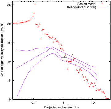
Radial velocities for 548 stars in the central region of 47 Tuc have been secured by Gebhardt et al. (1995), and the inferred velocity dispersion profile is plotted along with the older data in Fig. 1. This figure confirms the result that the central velocity dispersion may be considerably higher than in Meylan (1988).
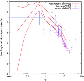
Line-of-sight velocity dispersion profiles of Meylan (1988), Gebhardt et al. (1995) and Lane et al. (2010). For the first of these the vertical error bars are as in the original publication, and the horizontal error bars give the range of projected radii in which the stars fall. For Gebhardt et al. (1995) we have copied curves in their figure which give estimates of the velocity dispersion profile and its 90 per cent confidence interval. For the most recent data set (Lane et al. 2010) we have copied the points and vertical error bars from their fig 11.
Recently, Lane et al. (2010) obtained a velocity dispersion profile based on the largest spectroscopic sample ever observed for 47 Tuc (see also Kiss et al. 2007; Székely et al. 2007), and we have included the results in the figure. Their results show that for the outer parts of the cluster the velocity dispersion appears to be rising with radius, while the central value (obtained by fitting a Plummer model) is only about 9.6 km s−1. Note, however, that one of the criteria for membership of 47 Tuc in their study was that the radial velocity must lie within a certain range of width about 45 km s−1 (their fig. 1). This would have excluded the two high-velocity stars discovered by Meylan et al. (1991), and probably suppresses the velocity dispersion at small radii. 25 stars which, according to the criteria of membership in Lane et al. (2010), are members of 47 Tuc actually lie outside the conventional tidal radius. Several of these extratidal stars lie in sparsely populated parts of the colour–magnitude diagram (their fig. 3), which suggests that they may not be members at all. It is possible that the membership criteria are insufficiently strict at large radii.
On account of such arguments, for the work reported here we have relied mainly on the data of Gebhardt et al., and so we now discuss it a little further. The sharp drop in the Gebhardt et al. data just inside 1 arcmin is interesting. Gebhardt et al. (1995) regarded it as a sharp rise (as the radius decreases), and suggested tentatively that it may indicate a central population of dark objects. The analysis of Gebhardt & Fischer (1995), however, implies that the M/L ratio inside this feature is little higher than at 5 arcmin. In fact, it implied that there was a zone of very low M/L ratio around 1 arcmin (presumably because the drop in velocity dispersion in this vicinity is almost Keplerian). Furthermore, the 90 per cent confidence limits on this result require an increase in M/L with increasing radius between about 1 and 4 arcmin. The lesson we draw from this discussion is that the features in the velocity dispersion profile may have little significance, and indeed the confidence limits themselves are subject to some doubt.
In our selection of models (Section 3) we have not used the wealth of data on proper motions (Rees 1996; King & Anderson 2001; McLaughlin et al. 2006), the bulk of which is confined to the innermost 100 arcsec. Nevertheless we shall compare some aspects of these data, such as anisotropy (Section 5.2), with one of our best models.
The rotation of the cluster is evident in both proper motions and radial velocities, and has been studied in many of the above papers. Unfortunately, however, our Monte Carlo technique is restricted to the case of spherical symmetry and no rotation. We return to this issue in Section 4.2.
2.2.3 Luminosity and mass functions
Ground-based data on the mass function (Hesser et al. 1987) provided an important constraint for the fitting of King-like models (Meylan 1989), and we shall see that luminosity functions continue to serve such a role in our work. Indeed, the use of the luminosity function is preferable, as it places the comparison closer to the observational domain, and simplifies problems connected with the mass–luminosity relationship. We have, however, mainly used more recent data: the luminosity functions derived from Hubble Space Telescope observations by Anderson & King (1996) at 1 and 14 core radii, where the core radius was taken to be 23 arcsec. The outer field goes down to magnitudes corresponding to stellar masses of about 0.1 M⊙. Other information on the luminosity function, though not used here, can be found in de Marchi & Paresce (1995), Santiago, Elson & Gilmore (1996) and Howell, Guhathakurta & Gilliland (2000).
We have retained the older data of Hesser et al. (1987) for one discussion in Section 4.3, where we consider their ‘composite’ luminosity function. As the authors themselves state, they did not attempt to correct for mass segregation when combining data secured at different radii, and it should not necessarily be regarded as a global luminosity function. Our interest in it is focused on the stars above turnoff, however.
2.2.4 Binary fraction
The binary fraction is very relevant for a variety of exotic objects, including blue stragglers and millisecond pulsars. Nevertheless, it seems to be observationally rather poorly constrained in most globular clusters, and 47 Tuc is no exception. The issue is complicated by mass segregation and the observational selection effects of the various techniques for detecting binaries.
From inspections of colour–magnitude diagrams, de Marchi & Paresce (1995) and Santiago et al. (1996) estimated that the fraction of ‘equal-mass’ binaries in fields 4.6 and 5 arcmin from the cluster centre was at least 5 per cent. Using the same basic approach, at the same distance of 4.6 arcmin, Anderson (1997) found a fraction of at most 2 per cent with mass ratio q > 0.5, in the magnitude range from V = 20.5 to 23.5. Again using broadly the same technique, Milone (personal communication) finds the fraction of binaries with q > 0.5 to be 0.015 ± 0.008, and the fraction of all binaries to be 0.026 ± 0.015. His measures refer to a region between 0.95 and 2.4 arcmin from the centre, and he points out that they take no account of the recently discovered intrinsic broadening of the main sequence (Anderson et al. 2009). In the central regions (< 90 arcsec) Albrow et al. (2001) estimated a binary fraction of about 14 per cent, based on observations of eclipsing binaries and some modelling. The stars observed range in V from about 16 to about 23, and it is known from modelling (e.g. Heggie & Giersz 2008a) that mass segregation is particularly pronounced among bright objects. Knigge et al. (2008) estimated a similar binary fraction among white dwarfs in the core.
Even though these estimates refer to somewhat different populations of binaries, and in some cases at different locations, the binary fraction seems to be the least well constrained of the observational quantities we have discussed.
2.2.5 Pulsars
It is estimated (Heinke et al. 2005) that 47 Tuc contains about 300 neutron stars. Among these are 23 observed millisecond pulsars (Freire et al. 2003).1 Since our modelling focuses on dynamical issues, the interest of these objects is twofold. First, some previous models of 47 Tuc have invoked such heavy remnants as being necessary to account for the central velocity dispersion (e.g. Meylan & Mayor 1986). Secondly, well-observed pulsars act as probes of the gravitational field (Phinney 1992), in a way that we now summarize.
16 of the millisecond pulsars have timing solutions which include measurements of the logarithmic period derivative  , where P is the pulse period. One contribution to this is intrinsic, caused by the spin-down of the pulsar, but the size of this contribution (which is positive) is estimated to be of the order of
  (Freire et al. 2001). In addition there is a Doppler contribution from the relative acceleration of the pulsar and the observer, and the main contribution is generally that due to the matter in the cluster itself. For a spherically symmetric cluster the magnitude of this term is GM(r) cos θ/(cr2), where M(r) is the cluster mass within the radius r of the pulsar, G, c are the usual physical constants and θ is the angle between the line of sight to the pulsar and the outward radial direction at its location in the cluster. Thus, the spin period of a pulsar located on the far side of the cluster appears to be decreasing, unless the contribution from intrinsic spin-down is too large. Of course, only the projected radius rp=r sin θ is known with any accuracy. For a given cluster model and given rp, however, the extreme values of the Doppler contribution can be calculated. Then, all observed values of
  should lie between these extrema, except for the small intrinsic contribution. This is illustrated for one of our models in Fig. 11.
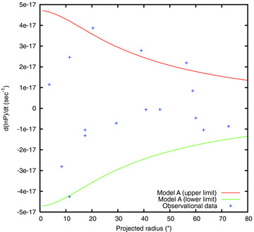
Comparison between spindown rates of millisecond pulsars (Freire et al. 2003) and the extreme contributions from the gravitational acceleration of Model A.
3 THE SIMULATIONS
3.1 Model description
As in previous papers in this series, the code we use is an updated version of the Monte Carlo code developed in Giersz (1998, 2001, 2006). It includes synthetic stellar evolution of single and binary stars using prescriptions described by Hurley, Pols & Tout (2000) and Hurley, Tout & Pols (2002). The only relevant updates to report here are the inclusion of (i) exchange interactions (through the use of cross-sections), and (ii) natal kicks for both neutron stars and black holes (which had been confined to single neutron stars in previous versions of the code).
For initial conditions we adopt the assumptions given in Table 1. The table also includes an indication of the range of numerical values which were explored in the search for a model which is described in Section 3.3. Some of our choices require a little elaboration here.
Choice of initial conditions, etc.
| Property | Distribution adopted | Parameter | Meaning | Range (small-scale models) | Range (full-scale models) | Notes |
| Number of stars | N | a | 1.8–2.2 × 10⁶b | |||
| Structure | King (1966) | W0 | Central potential | 4–11 | 7–10 | c |
| Tide | Giersz et al. (2008) | rt | Tidal radius | a | 72–116 pc | See text Section 3.1(iv) and d |
| Radius parameter | rt/rh | 25–500 | 21–60b | Determines rh (given rt) | ||
| Mass function | Two-part power law | m2 | Maximum mass | 2–150 M⊙ | 2–150 M⊙ | Kroupa (2008) but with |
| (single stars) | mb | Break mass | 0.86–0.9 M⊙ | 0.75–1 M⊙ | different parameter values | |
| m1 | Minimum mass | 0.1 M⊙ | 0.08 M⊙ | |||
| α2 | Upper index | 2.3–5.3 | 2.3–4.5 | Salpeter is 2.35 | ||
| α1 | Lower index | 0.4–1.3 | 0.4–1.3 | |||
| Binaries | Kroupa (1995) | fb | Binary fraction | 0–0.20 | 0–0.06 | See text Section 3.1(ii) |
| Mass segregation | None | But see the end of Section 4.2 | ||||
| Natal kicks | Gaussian | σ | One-dimensional dispersion | 190 km s−1 | 130–190 km s−1 | neutron stars and black holes |
| Age | 11 Gyr | 11–12 Gyr | ||||
| Metallicity | Z | 0.0035 | 0.003–0.0035 |
aSee text Section 3.3.
bLarger values were tried for truncated polytropic models.
cAlso Woolley (1954) and polytropic models (Section 4.2).
dA wider range was tried for truncated polytropic models.
The initial mass function (a two-part power law) depends on five parameters, but only four were adjusted in the search for a model. For the low-resolution initial search (Section 3.3) the minimum mass was held at m1 = 0.1 M⊙, as in previous papers in this series. It was kept at m1 = 0.08 M⊙ for the full-resolution models discussed in Section 4.
As in our work on M4 (Heggie & Giersz 2008a), the binary parameters follow the prescription of Kroupa (1995), except that the initial component masses are derived from the same initial mass function as the single stars in our model; its parameters normally differ in value from those in the mass function used by Kroupa. The component masses, period and eccentricity are then subject to ‘eigenevolution’ and ‘feeding’ algorithms. These have a physical basis and are designed to build in a number of correlations consistent with observational data.
For the initial spatial distribution we have adopted King models, but models which (in general) underfill the initial tidal radius. Thus there is a distinction between the tidal radius (determined by the strength of the tidal field and the mass of the cluster) and the edge radius of the King model. We have also experimented with several other types of model, as described briefly in Section 4.2.
A constant tidal field strength is used, as if the cluster were in a circular orbit. For 47 Tuc Tucholke (1992) and Dinescu, Girard & van Altena (1999) estimated an eccentricity of about 0.17, i.e. the Galactocentric distance varies by approximately this fractional amount on either side of its mean value. Therefore, our assumption has some approximate validity.
Though it is not strictly an issue of modelling, for the purposes of comparison between model and observations we need to choose values for the age and distance of the cluster. The adopted distance is the value given in Table 2, but for the main model described in Section 4 we found it slightly advantageous to choose an age at the upper end of the range in the table, i.e. 12 Gyr (see Section 4.5).
Data on 47 Tuc.
| RGC1 | 7.4 kpc |
 | 4.5 kpc |
| EB−V1 | 0.04 |
| [ Fe/H ]1 | −0.76 |
| Total mass M2 | 1.1 × 10⁶ M⊙ |
| Half-mass relaxation time trh1 | 3.0 × 10⁹ yr |
| Central relaxation time trc1 | 0.9 × 10⁸ yr |
| Age3 | 11+1−1× 10⁹ yr |
| r1c | 0.40 arcmin |
| r1h | 2.79 arcmin |
| r1t | 42.86 arcmin |
| RGC1 | 7.4 kpc |
| 4.5 kpc |
| EB−V1 | 0.04 |
| [ Fe/H ]1 | −0.76 |
| Total mass M2 | 1.1 × 10⁶ M⊙ |
| Half-mass relaxation time trh1 | 3.0 × 10⁹ yr |
| Central relaxation time trc1 | 0.9 × 10⁸ yr |
| Age3 | 11+1−1× 10⁹ yr |
| r1c | 0.40 arcmin |
| r1h | 2.79 arcmin |
| r1t | 42.86 arcmin |
Sources and notes: 1Harris (1996), updated on
http://www.physics.mcmaster.ca/~harris/mwgc.dat on 2010 January 19; 2Meylan (1989); 3Gratton et al. (2003), though their results have been simplified slightly.
Data on 47 Tuc.
| RGC1 | 7.4 kpc |
| 4.5 kpc |
| EB−V1 | 0.04 |
| [ Fe/H ]1 | −0.76 |
| Total mass M2 | 1.1 × 10⁶ M⊙ |
| Half-mass relaxation time trh1 | 3.0 × 10⁹ yr |
| Central relaxation time trc1 | 0.9 × 10⁸ yr |
| Age3 | 11+1−1× 10⁹ yr |
| r1c | 0.40 arcmin |
| r1h | 2.79 arcmin |
| r1t | 42.86 arcmin |
| RGC1 | 7.4 kpc |
| 4.5 kpc |
| EB−V1 | 0.04 |
| [ Fe/H ]1 | −0.76 |
| Total mass M2 | 1.1 × 10⁶ M⊙ |
| Half-mass relaxation time trh1 | 3.0 × 10⁹ yr |
| Central relaxation time trc1 | 0.9 × 10⁸ yr |
| Age3 | 11+1−1× 10⁹ yr |
| r1c | 0.40 arcmin |
| r1h | 2.79 arcmin |
| r1t | 42.86 arcmin |
Sources and notes: 1Harris (1996), updated on
http://www.physics.mcmaster.ca/~harris/mwgc.dat on 2010 January 19; 2Meylan (1989); 3Gratton et al. (2003), though their results have been simplified slightly.
3.2 Generation of observational data
We have already discussed (Section 2.2) the main kinds of observational data which we shall attempt to fit with our model. Here, we give the recipes used for the generation of the corresponding data from our model (and some additional data such as the core radius).
At any time, the output of the Monte Carlo model consists of a list of data for each star or binary. These data include the radius r (i.e. distance from the cluster centre), radial and tangential velocity (vr and vt), mass, V-luminosity LV in solar units and colour of the star. For binaries the same data are available for both components, along with the semimajor axis.
3.2.1 Surface brightness
 if r > d. The total surface luminosity density is the sum over all shells of radius r > d (which we also denote by ΣV in what follows), and then the surface brightness is given (in V magnitudes per square arcsec) by
This method has a disadvantage that the brightness is infinite along a line of sight such that d=r for some shell. It would be possible to construct a realization of the model by selecting the full position of each star at random on the corresponding shell, and then determine the surface brightness in a manner which is more akin to the observational approach. We have verified that this method produces similar results to the method described in the previous paragraph, and prefer that method (i.e. equation 1), as it has the merit of introducing no additional source of noise.
For the observational core radius we determine the smallest value of d such that the surface brightness is half that at the centre. (We also refer to a dynamical core radius in Section 5.5.)
3.2.2 Surface density profile, binary fraction and luminosity function
Our calculation of the surface density (i.e. number of stars per unit area on the sky) uses the same formulae as for surface brightness, as just described, except that LV is omitted, and the conversion is to number per square arcsec and not V magnitudes. For the (local) binary fraction we compute the ratio nb/(nb+ns), where nb is the projected density of binaries, and ns is the projected density of single stars. (Note, however, that the data in Table 4 give the global binary fraction.) The luminosity function is calculated in the same way as the surface density, but separates stars according to the appropriate magnitude bins.
Initial and present-day conditions for model A.
| t = 0 | t = 12 Gyr | |
| Na | 2.00 × 10⁶ | 1.85 × 10⁶ |
| Mass (M⊙) | 1.64 × 10⁶ | 0.90 × 10⁶ |
| Tidal radius (pc) | 86 | 70 |
| Half-mass radius (pc) | 1.91 | 4.96 |
| Half-mass relaxation time (Gyr) | 0.70 | 3.66 |
| W0 | 7.5 | – |
| Observational core radius (pc) | 0.42 | 0.55 |
| Binary fraction | 0.0220 | 0.0084 |
| Index of upper IMF | 2.8 | |
| Index of lower (I)MF | 0.40 | 0.36b |
| Minimum mass (M⊙) | 0.08 | |
| Break mass (M⊙) | 0.8 | |
| Maximum mass (M⊙) | 50.0 | |
| White dwarfs (M⊙) | 0 | 3.1 × 10⁵ |
| Neutron stars (M⊙) | 0 | 313 |
aNumber of single stars plus number of binaries.
bMeasured best fit between 0.3 and 0.8 M⊙, main-sequence stars only.
3.2.3 Profiles of line-of-sight velocity dispersion and proper motion
Consider the point on a shell of radius r at which it is pierced by the line of sight of projected radius d < r. We assume the transverse velocity of the star is randomly orientated in the tangent plane to the shell, and then it is easy to show that the mean square line-of-sight velocity is given by v2r(r2−d2)/r2+v2td2/(2 r2). For each shell within the line of sight, this expression is then weighted by the surface density of the star, i.e. by a factor  , and the weighted average gives the line-of-sight velocity dispersion.
For the line-of-sight velocity dispersion, stars fainter than absolute magnitude V = 6 are excluded from the sum. For proper motions similar formulae are used, with the appropriate magnitude limit (Fig. 12).
Anisotropy in the proper motions of Model A and the observational result for stars with mV < 18.5 within 100 arcsec (McLaughlin et al. 2006). The label on the ordinate specifies what is computed, the mean square radial and tangential proper motions at a particular line of sight being σ2R and σ2Θ.
3.2.4 Pulsar acceleration
For each line of sight, the line-of-sight component of the gravitational acceleration is computed at the location of each shell, and the maximum value found.
3.3 Finding a model
The starting point of our search for a model was a consideration of present estimates of the mass and dimensions of the cluster (Table 2). The half-mass relaxation time is long, which suggests that the cluster has not lost a very large fraction of its initial mass. Indeed, the formulae given by Baumgardt & Makino (2003) suggest that, even with its present mass, the dissolution time is of the order of 1011 yr. This in turn would suggest that most of the mass lost so far by 47 Tuc results from stellar evolution, and that its initial mass was less than twice its present mass. For much the same reason we began by assuming that its initial half-mass radius was not very different from its present value. Only in the core is the relaxation time short enough to suggest extensive evolution by relaxation.
In these small-scale models the age was taken as 11 Gyr, as in Table 2, and the minimum mass was taken to be 0.1 M⊙. These values differ from the values of 12 Gyr and 0.08 M⊙ adopted for the main model in Section 4, but the resulting differences are negligible for the purpose of the explorations discussed here. These models can be scaled to any value of N, which is not an input parameter of the model and is therefore not given in Table 1. Similarly we do not specify the range of rt for these models, as this also depends on the chosen scaling.
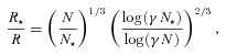
Our first finding was that the canonical values for the initial mass function did not provide a satisfactory fit to the luminosity functions which we were trying to match (see Section 2.2.3). We found that all our subsequent modelling of the luminosity functions (at least, below the turnoff) was satisfactory if we chose values closer to α1 = 0.5 and mb = 0.9 M⊙, where these parameters are defined in Table 1. (Nevertheless, slightly different values were eventually adopted for the model presented in Section 4; see also Section 4.5.) Thus, the low-mass initial mass function is flatter than in the canonical formulae of Kroupa (2008). Strictly, only the value of α1 is approximately determined by this comparison; all we can say of mb is that it is not much below the present-day turnoff mass, and the value chosen merely represents approximately the most modest change from the canonical values.
Our conclusion about α1 seems quite robust, and is illustrated in Fig. 2. This shows a scaled version of a model close to the one to be presented in Section 4, and one with identical parameters (see the caption to the figure and Table 3) except for the slope of the lower part of the IMF. Though a better fit could certainly be obtained by varying more than just one parameter, the figure does serve to illustrate the effect of a mismatch in the choice of IMF.
Observed luminosity functions at two radii (from Anderson & King 1996) compared with two models. One is a scaled version of a model close to that presented in Section 4, scaled to N* = 40 000, and the other is an identical model except for the power-law index of the lower initial mass function, which is the ‘canonical’ value of 1.3 (Kroupa 2008). The actual initial parameters for the first model are given in Table 3.
An approximate small-scale model.
| Parameter | Initial value |
| Number of stars | N* = 40 000 (N = 2 × 10⁶) |
| Total mass (M⊙) | 2.93 × 10⁴ (1.47 × 10⁶) |
| Tidal radius (pc) | 295 (109) |
| Half-mass radius (pc) | 6.6 (2.4) |
| Central potential of King model (W0) | 8 |
| Binary fraction | 0.02 |
| Upper mass function index | 3.3 |
| Lower mass function index | 0.5 |
| Minimum, break and upper mass (M⊙) | 0.1, 0.9, 50.0 |
Note: Corresponding values for a full-scale model, where these are different, are given in brackets.
In order to give a flavour of how our search for a model proceeded from this point, we now explore a coarse grid of the main initial structural parameters, namely the initial half-mass radius and concentration. [We adopt the models of King (1966) for the initial structure.] All the models in this particular discussion use a relatively large initial value of the tidal radius (r*t = 500 pc, where we give the value for the small-scale model.) It should also be said that they represent a tiny subset of all the models we explored (see Table 1).
Some results of this representative mini-survey are summarized in Fig. 3. The results of each model were scaled (by the particle number) to fit the central surface brightness of 47 Tuc, and then this figure gives the line-of-sight velocity dispersion at a projected radius of 1 arcmin. While these suggest that there is a range of relatively compact initial conditions (r*h in the range from 1.5 to 2 pc) yielding approximately the correct velocity dispersion (see Fig. 1), further inspection reveals serious problems.
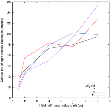
Line-of-sight velocity dispersion at 1 arcmin for a number of scaled models. Different curves correspond to different initial concentrations. The abscissa is the initial half-mass radius of a small-scale model with N* = 104 stars, and is related to that of a full-scale model with N stars by equation (2). The models have been scaled to the correct central surface brightness for 47 Tuc, and so the value of N differs from one model to another.
Figs 4 and 5 compare the entire surface brightness and velocity dispersion profiles for the model with initial concentration W0 = 9 and scaled initial half-mass radius 2 pc. It has been scaled to a system with N = 2 × 10⁶ stars. While the central surface brightness and velocity dispersion at 1 arcmin match reasonably well, as required, the remainder of the profiles do not match 47 Tuc at all. The surface brightness of the halo is too low, and the same result is obtained if one checks star counts (Da Costa 1982). The model does, however, have nearly the correct core radius. The poor match of the velocity dispersion profile is even more revealing. The deficiency at large radii may be attributable to the undermassive halo, as shown by the surface brightness profile. The rise in the velocity dispersion well inside the core radius, however, is in complete contrast with the observational result. This reveals the presence in the model of a segregated population of massive objects.
Surface brightness profile of a scaled model compared with the composite profile of Trager et al. (1995).
Line-of-sight velocity dispersion profile of a scaled model compared with the observational results of Gebhardt et al. (1995). The spike in the model is attributable to a single star at small radius. Only bright stars, with V < 5, were included.
As an aside, we consider briefly the nature of this population. Because of the scaling, the model has a low escape velocity, though the velocity dispersion of natal kicks (of black holes and neutron stars) was unscaled, and so, not surprisingly, the population of neutron stars is very small. The compact central population consists almost entirely of white dwarfs, which make up 49 per cent of the entire mass of the cluster. There is nothing abnormal about this, especially given the relatively flat low-mass initial mass function, which substantially decreases the mass of the main sequence below turnoff. In our favoured model, however (see Table 4), the white dwarf mass fraction is only 34 per cent, and the central velocity dispersion agrees better (Fig. 8).
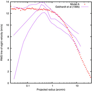
Line-of-sight velocity dispersion profile of Model A compared with the 90 per cent confidence band estimated by Gebhardt et al. (1995).
Returning to the problem of finding a suitable scaled model, we can also view the results of this mini-survey from a different angle; and it turns out to be a more fruitful approach. Instead of scaling to match the central surface brightness, consider the result if instead one scales to match the central line-of-sight velocity dispersion. Then it is found that the resulting models are too faint centrally, and the (observational) core radius is too large, no matter how compact the initial conditions are. A better fit could therefore be obtained if expansion of the core could be suppressed. Various mechanisms are known to cause expansion of the core, including loss of mass by stellar evolution, binary heating and the action of black holes. (The papers by Chernoff & Weinberg (1990), Heggie, Trenti & Hut (2006) and Merritt et al. (2004), respectively, may serve as samples of the extensive literature on these processes.) We judge that the initial binary fraction adopted here (2 per cent) is too low (for our choice of initial period and mass distributions) to cause significant core evolution; in any case the observational constraints (Section 2.2.4) do not suggest that it can be much lower, and so we have not attempted to reduce the binary fraction. The remaining mechanisms for core evolution, however, all involve the more massive stars in the initial mass function, and we have considered modifications here.
Despite its implausibility, perhaps, our efforts initially focused on truncation of the high-mass IMF, by severely reducing m2 (Table 1). Indeed values around 2 M⊙ gave rather satisfactory scaled models, without any change in the slope of the upper mass function from the canonical value of 2.3. One problem with such a mass function is that no neutron stars are formed, and so we explored different ways of altering the IMF. Though any significant increase in the break mass always gave poorer results, results were almost as good if we raised the maximum mass again but compensated by steepening the power-law index of the upper mass function.
With only small changes in the remaining parameters, the parameter values arrived at in this way led to the small-scale model specified in Table 3. Then, with further changes and much experimentation, we arrived at the full-scale model described in the next section. We summarize in Table 1 the entire ranges of all parameters which we explored, both with small-scale models (i.e. as described in this section) and with full-scale models (as in Section 4). We do not intend to suggest that all possible joint variations in these parameters were investigated; very often the extreme values in these ranges were tried only for one or very few choices of the remaining parameters. In principle, it would be desirable to adopt a more systematic way of searching this rather large parameter space. Harfst, Portegies Zwart & Stolte (2010) describe an N-body study of the Arches cluster which illustrates such an approach, at least when adjusting a pair of parameters (in their case the initial virial radius and particle number.)
4 A MODEL OF 47 TUC
Unlike the models discussed in the previous section, the model we are about to present is a full-scale model of 47 Tuc. It will be seen that the profiles and other data are considerably smoother than for the models discussed hitherto. This standard model will be referred to as Model A. Details of its initial specification, along with a summary of conditions at 12 Gyr, are given in Table 4. Though the slope of the upper mass function may seem steep, still higher values (in the range 3.75–4.5) were inferred by Meylan (1989). His result was based on the need to produce the appropriate mass of white dwarfs to account for the velocity dispersion profile. Our motivation is rather different, as we have already mentioned at the end of the last section. Meylan, incidentally, took a much more nearly canonical value for the power-law index of the lower mass function than ours (he took 1.2), but a similar break mass (he took 0.88 M⊙).
It may be of interest to note that each full-sized model such as this takes less than a day on a single Dual-Core AMD Opteron 2214 at 2.2 GHz.
4.1 Surface brightness and density profiles
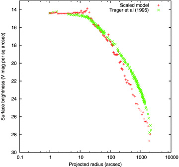
As can be seen in Fig. 6, model A is somewhat bright at small radii. Quantitatively, our central value is about 14.1 in the units of the figure, while fits by Trager et al. (1995) and McLaughlin et al. (2006) give values of 14.42 and 14.26, respectively. Less evident, perhaps, because of the steepness of the profile at large radii, is the fact that the model is too faint there. The mismatch approaches about 1 mag at the largest radii plotted (though this is less severe than for the scaled survey model shown in Fig. 4) and can be at least partially attributed to our treatment of the tide (see text below).
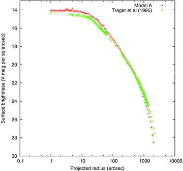
Surface brightness profile of Model A compared with the composite profile of Trager et al. (1995).
Star counts offer an alternative approach to the comparison of the spatial structure of the model with 47 Tuc (Fig. 7). The model is somewhat overdense at small radii. If the cut-off in V of the star counts is determined from synthetic model data, as described at the end of Section 2.2.1, the mismatch is approximately 0.1 dex. This is approximately compatible with the excess brightness discussed above.
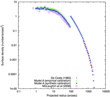
Surface density profile of Model A compared with some of the star counts of Da Costa (1982), which have a limiting apparent magnitude of mV = 19.45, and the surface density of stars above turnoff from McLaughlin et al. (2006). Details of the ‘calibration’ are given in Sections 2.2.1 and 4.1. For the model, we switch from one limiting magnitude to the other at 100 arcsec.
At large density, however, the evidence from surface density gives a different impression from the surface brightness, as the fit with the observational data is now much better. Though the fit is still imperfect, it was evidence like this which for us confirmed the possibility that the composite surface brightness profiles might not be very reliable at large radii. We had been alerted to this by finding models which produced satisfactory mass functions (to judge by luminosity functions below the luminosity of the turn-off) but which seemed faint at large radii when judged by the surface brightness profile.
Our treatment of the tide (Giersz et al. 2008) is a further complication, as it implies that the most distant star actually lies some distance inside the tidal radius. For this reason, the fact that the surface density distribution of the model still falls below the observations at large radii is not necessarily a significant issue.
4.2 Velocity dispersion profile
This, presented in Fig. 8, is perhaps the most unsatisfactory comparison for this model. Whatever the formal statistical result (by comparison with the 90 per cent confidence band estimated by Gebhardt et al. 1995), and however much it improves on the model shown in Fig. 5, it still gives the qualitative impression of not conforming to the shape implied by the observations. This is particularly noticeable in three places: at the smallest radii, where it might seem too high, and around 2 and 10 arcmin, where the model velocity dispersion seems too high and too low, respectively. Besides possible shortcomings of the model, a number of relevant factors should be borne in mind, and we consider them in turn.
Looking first at small radii, up to about 0.5 arcmin, we see that any well-fitting model with a relatively flat (or, at least, non-increasing) velocity dispersion profile must pass close to the 90 per cent confidence limits at very small radii and/or around 0.4 arcmin. Therefore, the fact that our Model A does so does not cast doubt on its correctness.
The second point to note is that, as mentioned in Section 2.2.2, our model takes no account of the rotation of the cluster. The maximum mean line-of-sight (rotational) velocity, about 6.5 km s−1, occurs at a radius of about 5–6 arcmin (Meylan & Mayor 1986); the Fabry–Perot observations of Gebhardt et al. (1995, their fig. 11) extend out to slightly smaller radii, but they give a value above 7.5 km s−1 already at about 4 arcmin. Thus, the rotation is large in the second of the three regions where the mismatch seems most pronounced. The influence of rotation may also extend to larger radii: it is worth noting that the single mass, rotating Fokker–Planck cluster models of Kim et al. (2008, their figs 1, 11 and 12) clearly show that rapidly rotating clusters evolve faster and have larger half-mass radii than non-rotating clusters. This will put more mass into the outer parts of a cluster, and increase the velocity dispersion there.
The third factor to bear in mind is the influence of the tide at large radii. We treat its action as a cut-off, which is an increasingly rough approximation as the tidal boundary is approached. [The observations of Gebhardt et al. (1995) extend to almost half the observed tidal radius.] It has been known since the work of Drukier et al. (1998) that the velocity dispersion profile in some clusters flattens off towards the tidal radius, presumably because of the effects of the galactic tide. Such an effect is certainly observable in N-body simulations (e.g. Giersz & Heggie 1997; Capuzzo Dolcetta, Di Matteo & Miocchi 2005; Küpper et al. 2010) and has also been confirmed recently for 47 Tuc by Lane et al. (2010) (see Fig. 1). Therefore, the apparently excessively rapid decline of the velocity dispersion at large radii in the model may be an artefact of our simple tidal treatment. We note in this respect that the multi-mass anisotropic King model of Meylan (1988) did a much better job in fitting the outer velocity dispersion and its trend. The very large half-mass radius in that model (Section 5.1) is no doubt a factor, placing more mass at large radii and elevating the velocity dispersion there. The fact is, however, that our models, which start as compact King models, do not evolve as far as those constructed by Meylan. Also, it seems likely that some of the velocity dispersion which Meylan's model fitted is due to processes which were not included in that model, i.e. the tidal field.
It is worth reporting here that we have attempted, with very limited success, to improve the outer velocity dispersion by constructing models which might enhance the mass density at large radii. In particular we tried:
Woolley models (Woolley 1954), which employ a truncated isothermal distribution, in contrast to the lowered isothermal distribution of the King model; their concentration can be specified in much the same way, i.e. by the scaled central potential W0;
polytropic models, with polytropic index exceeding the Plummer value of 5; the models were truncated at the tidal radius and revirialized globally, just as would be done with a Plummer model;
initially mass segregated models generated according to either (a) the prescription given by McMillan & Vesperini (2007), with time delay of stellar evolution up to 250 Myr; or (b) the method of Baumgardt, De Marchi & Kroupa (2008a), with mass segregation down to 2 M⊙.
Mass-segregated models do differ in the central part of the system, generally slightly lowering the velocity dispersion, but in the region farther out than about 5 arcmin they are indistinguishable from models without primordial mass segregation. Polytropic models in particular provided a slightly better fit to the velocity dispersion profile, though the improvement is too marginal to justify abandoning King initial conditions.
4.3 Luminosity and mass functions
Luminosity functions in fields at two radii are shown in Fig. 9, in comparison with data from Anderson & King (1996). According to those authors, turnoff corresponds to about V = 4.1 on the scale of this diagram. Below turnoff, then, the agreement is fairly satisfactory in both fields, in terms of both overall shape and normalization. The quality of the normalization is relevant to the discussion in Section 4.1. For instance, the inner field is at a radius of about 23 arcsec where, as we have seen, the evidence of both number counts (for stars above turnoff) and surface brightness is that the model is too dense or bright by about 0.1 dex. Nevertheless, the mean difference in the logarithm of the luminosity function in Fig. 9 between V = 4 and 8 is 0.02 ± 0.03 (standard error), i.e. the model is not significantly denser than the observations.
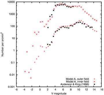
Luminosity functions at two radii, in Model A and from the observational data of Anderson & King (1996). Note that these authors specify the radii in terms of the core radius (1 and 14rc), and we have assumed rc = 23 arcsec.
This discussion is complicated by the fact that the data of Anderson & King (1996) do not extend much above turnoff, whereas the surface density data discussed in Section 4.1 are confined to stars above turnoff, and they also dominate the surface brightness. To explore the luminosity function above turnoff, in Fig. 10 we compare our global luminosity function with the composite luminosity function of Hesser et al. (1987). We have somewhat arbitrarily normalized the latter (by eye) in the upper main sequence, where we know from the evidence of Fig. 9 that the model appears to be satisfactory. A satisfactory match continues up to about the prominent peak (at the location of the horizontal branch), but no further. Actually, the distribution along the giant branch is known to be a sensitive test of stellar evolution (Bergbusch & VandenBerg 2001), complicated in 47 Tuc by the spatial variation of the giant branch itself (Freeman 1985; Bailyn 1994). Though we therefore make no attempt to resolve the mismatches in this brightest part of the luminosity function, it plays a significant role in the surface brightness, and problems here may well contribute to the fact that the surface brightness and density of the model appear to be excessive.
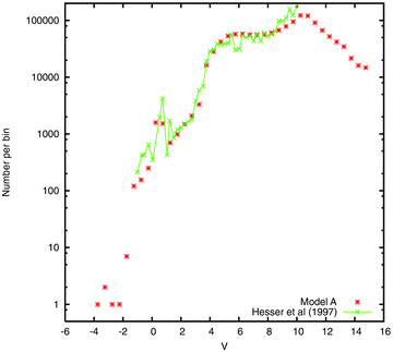
The global luminosity function of model A in comparison with that of Hesser et al. (1987). The latter has been normalized to give a reasonable fit in the upper main sequence.
Let us return again to a consideration of stars below turnoff. The low-mass mass function is often discussed in terms of the power-law index over some convenient mass range. We have preferred to carry out the comparison in the observational domain, i.e. in terms of the luminosity function, partly because the mass range over which the power law is fitted varies from one author to another, and partly because it is not always clear how the fit is actually carried out. In any event, such comparisons depend on the choice of mass–luminosity relationship. Nevertheless, we give one example, which is a comparison with the ground-based result of Hesser et al. (1987) for the global mass function. They found an index of 1.2 ± 0.3 (Salpeter = 2.35) for masses corresponding to 5 ≲V≲ 9, which corresponds to masses between about 0.5 and 0.8 M⊙. We find at least that an index of 0.9 provides a reasonable fit in this range. Nevertheless, a smaller value provides a better fit (in our model) if the range is extended to include more of the lower main sequence (Table 4). Indeed, the change from the primordial value is less than 0.1. Baumgardt & Makino (2003) used N-body models (not specifically geared to 47 Tuc) to assess the dependence of the mass-function index on mass lost by the cluster; and our result is entirely consistent with their fig. 9, since in our model 47 Tuc has lost less than half of its initial mass.
4.4 Pulsar accelerations
Fig. 11 shows that the model is very nearly consistent with observations of the spin-down of pulsars in 47 Tuc. The fact that three lie just above the upper curve is consistent with estimates of the small intrinsic component (Section 2.2.5). The critical object in this plot is the pulsar with the largest negative period derivative. It is known as 47 Tuc S (Freire et al. 2003), and these authors showed that it implies a projected mass/light ratio M/L > 1.4 in the region of the pulsar. In fact, the projected value of M/L at the location of this pulsar in our model is about 1.1. Note, however, that our model is a little bright in the core (Section 4.1), which depresses the value. (Incidentally, the projected value of M/L increases from this central value to about 2.3 at large radii; the global value is about 1.52.) Generally speaking, the tension between the requirements of the central surface brightness, on the one hand, and the acceleration of 47 Tuc S, on the other hand, was the single most important constraint in our attempts to find a satisfactory model.
4.5 Variation of parameters
Even though we had to work very hard to reach Model A, and discarded numerous models in the process, we can make no claim to the uniqueness of the model presented above, even within the limitations of the parameters which characterize our initial conditions. But in this section we wish to summarize the most notable changes (in the surface brightness, surface density, velocity dispersion profile, mass functions and pulsar accelerations) which occur if we adjust our choice slightly. The list of parameters begins with those in Table 4, but we have also considered a number of other possibilities, which are included in the list below. Where we have varied a given parameter, the values of the remaining parameters are fixed and close to, but not always exactly the same as, those in Model A. Where no mention is made of changes, it means that the changes (in the five quantities listed above) are negligible in comparison with other entries. We generally desist from giving a theoretical interpretation of these empirical statements, each one of which might be a research project on its own.
N (Initial number of stars): an increase by 5 per cent leads to an increase in the velocity dispersion by about 3 per cent, and an increase in the maximum gravitational pulsar spinup by about 4 per cent.
rt (Initial tidal radius): an increase by about 25 per cent leads to a decrease in the central surface brightness by about 0.3 mag and a corresponding decrease in the luminosity function in the inner field, an increase in the outermost radius in the surface brightness and density profiles by about 10 per cent, a decrease in the central line-of-sight velocity dispersion by about 5 per cent and a decrease in the maximum gravitational pulsar spinup by about 25 per cent. Note that, because we hold the initial ratio of tidal and half-mass ratio constant, a variation of the initial value of rt also affects that of rh.
rt/rh (Initial ratio of tidal and half-mass radii): an increase by 12.5 per cent (i.e. a correspondingly more compact initial configuration, relative to the tidal radius) gives an increase in the central surface brightness by about 0.1 mag per square arcsec, an increase in the central velocity dispersion by about 4 per cent and an increase in the maximum gravitational pulsar spinup by about 18 per cent.
W0 (Initial King concentration): an increase by 1 leads to an increase in the maximum gravitational pulsar spinup by about 14 per cent, but no other significant changes. This is also discussed in Section 3.3 (see especially Fig. 3).
fb (Initial binary fraction): an increase by 50 per cent (e.g. from 0.02 to 0.03) leads to a decrease in the central surface brightness by about 0.3 mag, a decrease in the central surface density by about 19 per cent and a decrease in the maximum gravitational pulsar spinup by about 11 per cent.
α1 (Index of the lower initial mass function): an increase by 0.1 (e.g. from 0.4 to 0.5) decreases the velocity dispersion profile by about 2 per cent, and causes small changes in the outer luminosity function as expected from the discussion in Section 3.3 (see especially Fig. 2).
α2 (Index of the upper IMF): an increase by 0.2 (e.g. from 2.8 to 3.0) leads to an increase in the central surface brightness by about 0.4 mag, an increase in the central surface density by about 0.15 dex and an increase in the maximum gravitational pulsar spinup by about 18 per cent.
mb (Break mass): an increase from 0.75 to 0.85 M⊙ leads to a decrease in the central surface brightness by about 0.6 mag, a decrease in the central surface density by about 30 per cent, some changes (in line with naive expectations from the change in break mass and the smaller central surface density) in the inner luminosity function and a decrease in the maximum gravitational pulsar spinup by about 20 per cent.
m1 (Minimum initial mass): we did not experiment widely with this parameter, but can report that an increase from 0.08 to 0.1 M⊙ causes an increase in the core velocity dispersion by about 2 per cent.
m2 (Maximum initial mass): a change from 50 to 150 M⊙ leads to negligible changes.
t (Time [Age]): an increase by 1 Gyr leads to a decrease in the central surface brightness by about 0.15 mag, a decrease in the central surface density by about 20 per cent and a decrease in the velocity dispersion by about 6 per cent.
D (Distance): an increase by 0.5 kpc leads to a corresponding reduction in the apparent length-scale of the surface brightness, surface density and velocity dispersion profiles, and an increase in the inner luminosity function by about 8 per cent.
Z (Abundance): an increase by 0.0005 from 0.003 to 0.0035 leads only to a decrease in the maximum gravitational pulsar spinup by about 4 per cent.
σk (One-dimensional dispersion of natal kicks of neutron stars): a decrease from 190 km s−1 (our canonical value) to 160 km s−1 leads to no significant changes, but a larger decrease to 130 km s−1 leads to an increase in the maximum gravitational pulsar spinup by about 10 per cent.
5 DISCUSSION OF THE MODEL
5.1 The size of 47 Tuc
A description of the spatial structure of globular clusters is often reduced to just three values: the core, half-mass and tidal radii. Our value for the tidal radius (Table 4) is rather comparable with those of Meylan (1988, about 70 pc) and Table 2 (which converts to 56 pc at the stated distance). Our value for the observational core radius (Table 4) is quite similar to that derived from Table 2, i.e. 0.52 pc. There is, however, an amazing variation in quoted values for the half-mass radius. Data in Table 2 lead to a value of about 3.65 pc, and the difference from our value (Table 4) may be explicable if the former value should really be understood as a projected half-light radius. The values in Meylan's best models, however, lie close to 9.5 pc, and we have no explanation for such a wide disagreement. It does, however, have the effect of placing more mass at larger radii in his model, and this may be one reason why his fit with the velocity dispersion profile at large radii is more successful than ours (see Section 4.2.)
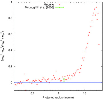
5.2 Velocity anisotropy
The velocity anisotropy of 47 Tuc near the centre has been constrained observationally by King & Anderson (2001) and McLaughlin et al. (2006). The former authors also measured anisotropy at about 4 arcmin from the cluster centre, but gave no quantitative results. Fig. 12 shows anisotropy among bright stars (V < 6) in our model, compared with the result for the brightest stars (mV < 18.5) within about 100 arcsec of the centre (McLaughlin et al. 2006). Though the observational result differs only marginally from zero, the results are consistent. A rapid rise at large radii, as seen in our model, is qualitatively consistent with what was inferred indirectly by Meylan (1988) on the basis of model fitting.
5.3 The binary frequency
Fig. 13 shows the radial distribution of the fraction of main-sequence binaries. This was calculated as in Section 3.2.2, except that in calculating the surface density of single stars we include only main-sequence stars, and in the surface density of binary stars we include only binaries in which both components are main-sequence stars. In both cases also the apparent V magnitude was limited to the range 20.5 to 23.5. These are quite appropriate choices for comparison with the observational data summarized in Section 2.2.4, except that the range of magnitudes used by Milone et al. (2008) was a 3-mag range specified in I. In the radial range of their data, our result is just consistent with theirs.
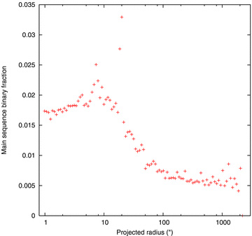
Projected fraction of main-sequence binaries (as defined in the text) in Model A. The high points are an artefact of the way in which the surface density is computed, which can be very large if the line-of-sight nearly coincides with the radius of a binary.
Of greater relevance for dynamics is the fraction of all binaries, not just those with main-sequence components. Our initial conditions generate a large proportion of relatively soft pairs. These are quickly destroyed, and the global fraction decreases by over 60 per cent (Table 4). Within the innermost 1000 stars, however, the binary fraction increases with time as recorded in Fig. 14, because of mass segregation.
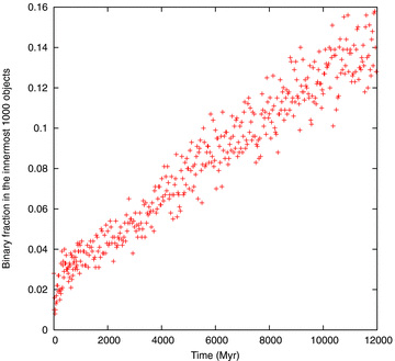
Fraction of all binaries in the innermost 1000 objects in Model A.
5.4 The dynamical role of dark remnants
In the core, the velocity dispersion in the model is certainly affected by degenerate components, which make up about 51 per cent of the mass there, but their mass fraction decreases at larger radii to give a global ratio of about 34 per cent (see Table 4). At face value, our result for the core contrasts with the finding of McLaughlin et al. (2006), who suggested, on the basis of the profile of dispersion of proper motions, that the contribution of heavy remnants (such as neutron stars and white dwarfs) is only a fraction of a per cent. The resolution of this discrepancy may simply be to understand that their estimate applied only to neutron stars, and perhaps the most massive white dwarfs. Our global result is comparable to a number of earlier estimates, based on model fitting, which were summarized by Heggie & Hut (1996).
Despite our tinkering with the initial mass function, and despite giving natal kicks with a one-dimensional dispersion of 190 km s−1, our model appears to produce a reasonable number (213) of neutron stars. A recent indirect estimate, based on a quite simple demographic argument, puts the total neutron star population in the cluster at ‘∼300’[Heinke et al. (2005); see also Verbunt & Meylan (1988)]. It has been argued (Ivanova et al. 2008) that substantial numbers of neutron stars must be formed in processes leading to smaller natal kicks than assumed in our model, and so the number in the model could well be larger if this refinement were added.
In our model there are only 19 stellar mass black holes at the present day, and their total mass is small compared with that of other remnants. The maximum number present at early times is over 1000, but the number falls to less than 40 within the first 30 Myr.
There is no sign of any early phase of runaway coallescence in the model. The results of Portegies Zwart & McMillan (2002, their equation 17), based on theory calibrated by N-body models up to N = 64k, imply that the collision rate is less than 1 per Myr. They also noted, however, that their result is likely to be an overestimate at half-mass relaxation times above about 30 Myr. Furthermore, our upper mass function is steeper than theirs, and this helps to diminish the rate of collisions. Incidentally, the initial half-mass density, which is 0.28 × 10⁵, is within the range of a number of young massive clusters at the present day (Portegies Zwart, McMillan & Gieles 2010).
5.5 The dynamical status of 47 Tuc
Because of its high concentration, it is tempting to assume that 47 Tuc is close to core collapse. Though it is a massive cluster, its core relaxation time is given (Harris 1996) as trc≃ 9 × 10⁷ yr. For an equal-mass King model having the same concentration as 47 Tuc at the present day, i.e. about 2.03, the core-collapse time is about 400trc (from data in Quinlan 1996). But it is known (e.g. Chernoff & Weinberg 1990) that the time to core collapse in systems with unequal mass is much smaller than that in equal-mass systems; these authors quote an example of a W0 = 7 King model, where a multi-mass system collapses in a time smaller than an equal-mass system by a factor of approximately 45. Putting all these factors together suggests that, indeed, the core of 47 Tuc should collapse within about 1 Gyr. The large numerical factors involved, however, suggest that this argument is quite precarious.
The spatial evolution of Model A is shown in Fig. 15. The core radius is represented by the two curves, one of them quite wavy, near the bottom of the figure, not far from the 1 per cent Lagrangian radius. These two curves are Bezier fits to rather noisy data on the core radius (cf. Fig. 16) generated in two ways. The curve labelled in the key as ‘dynamical’ is determined from the mass-weighted three-dimensional velocity dispersion and density of the innermost 20 particles, using the formula r2c = 3〈v2〉/(4πGρ0). The ‘observational’ curve is determined from a computation of the surface brightness profile, and is the radius at which this falls to one half of its central value (Section 3.2.1).
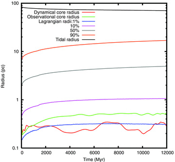
Evolution of Lagrangian, tidal and core radii in Model A. Definitions of the core radii are given in the text.
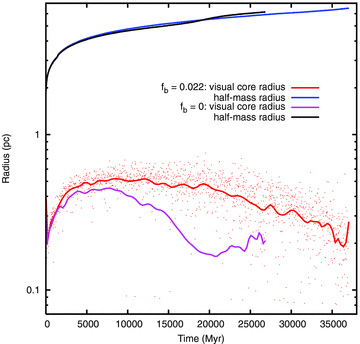
Evolution of half-mass and observational core radii in Model A and in a model with no primordial binaries but which is otherwise identical. The core radii are smoothed, but the original model data are also shown for Model A. Both runs were stopped at the point where the data ends.
We first notice that, except at the very start, there is a fairly steady (though decelerating) increase in the observational core radius, at least in absolute terms. It also increases relative to the dynamical core radius within the first few Gyr. We interpret the increase relative to the dynamical core radius as due to a combination of stellar evolution and mass segregation: as the turnoff mass decreases, the observable core is determined by stars of lower mass, which are more spatially dispersed. Hurley (2007) has described a similar effect in N-body simulations, but attributed it to the core collapse of the heavy (and presumably dark) stars. Perhaps both effects are present, or perhaps they are simply somewhat different descriptions of the same processes.
After the first few hundred Myr, the dynamical core radius is almost constant in absolute terms, but does appear to decrease slowly with respect to the half-mass radius (Fig. 15). The time-scale of this process, which we refer to as core collapse, is difficult to estimate from Fig. 15, but the predicted future evolution is given in Fig. 16. Evidently the collapse of the core slowly accelerates, but continues for at least a further 25 Gyr! On this evidence, then, 47 Tuc is far from core collapse.
Now we turn to the mechanism which causes the overall expansion of the system, the fact of which is evident from Fig. 15. Three processes come to mind:
mass loss from stellar evolution;
primordial binaries;
new binaries, formed in three-body interactions.
Empirical evidence comes from a comparison simulation in which the initial binary fraction was 0 (Fig. 16); we refer to this as Model A0. The half-mass radius increases at almost the same rate in both models, even though Model A0 contains at most one binary (formed in three-body interactions) until it reaches an age of about 23 Gyr (a few Gyr after the estimated time of core bounce, at about 20 Gyr). There are no binaries in it between about 500 Myr and 4 Gyr, and yet the expansion of the half-mass radius of Model A0 is very close to that of Model A, even during this period. It must be concluded, therefore, that the effect of binaries is almost negligible in both models, and almost the entire expansion must be due to mass loss from stellar evolution, at least up to an age of 12 Gyr.
The difference between the two models is more noticeable in the core, however, and we conclude that the core of 47 Tuc would be about 20 per cent smaller were it not for the action of the primordial binary population. In Model A0 it seems clear that the core radius has passed its maximum by an age of 8 Gyr, and the figure shows that core collapse is arrested at about 20 Gyr. From then on three-body binaries form in greater abundance, and there is a slight but noticeable acceleration in the expansion of the half-mass radius.
It may seem surprising that mass loss from stellar evolution is dominant. Its time-scale, however, is set by astrophysics. The other possible competitors (core collapse, and heating by primordial binaries) scale with the relaxation time, other things being equal. This time-scale increases with the mass of the cluster, and so for a sufficiently massive cluster, these stellar dynamical processes are relatively weak. 47 Tuc ranks fifth among the globular clusters of the Galaxy for luminosity (Harris 1996), and, given the rather narrow range of M/L ratios, is certainly one of the most massive.
It is an interesting and puzzling fact that the most luminous Galactic globular clusters tend to be the most concentrated (van den Bergh 2003). It is puzzling because, if we ignore stellar evolution, we expect the clusters of lowest mass to evolve fastest and therefore to approach or enter core collapse sooner; and this is the opposite of what is found. We see from this model of 47 Tuc, however, that high concentration is not necessarily any indication that the cluster is close to core collapse.
5.6 Missing ingredients
Several realistic aspects of star cluster evolution are omitted from our modelling. These include rotation, oblateness effects, a time-dependent tide (due to the ellipticity of the Galactic orbit of the cluster), tidal accelerations (as opposed to a cut-off), various aspects of binary dynamics (because we use cross-sections for the interactions) and the complexities of initial conditions. Some of these omissions are common to virtually all simulations of star cluster dynamics, and have been since the field began. At the present day, however, especially in the context of globular star clusters, it is the question of initial conditions which is most controversial and most fluid.
Initial conditions are complicated by a number of factors, of which we highlight two. The first is early gas expulsion. This has been the subject of considerable research for some time now (e.g. Geyer & Burkert 2001; Fellhauer & Kroupa 2005; Bastian & Goodwin 2006; Goodwin & Bastian 2006; Marks, Kroupa & Baumgardt 2008; Baumgardt, Kroupa & Parmentier 2008b), but we have ignored its effects. The second problem is that it has to be recognized that 47 Tuc cannot really be regarded as consisting of a single stellar population any more (Anderson et al. 2009). The appropriate paradigm for this situation, let alone its simulation, is full of uncertainties (Downing & Sills 2007; D'Ercole et al. 2008; Choi & Yi 2008).
Faced with these complexities one might conclude that a modelling exercise like that in the present paper is meaningless, misguided or at least premature. Our view on this is based on the fact that these missing features may affect only the first hundred million years of evolution, and perhaps less. We make the assumption that our models, after such a period of evolution, do resemble hypothetical models which start with different initial conditions but do include these missing ingredients. Thus, Marks et al. (2008) have shown that models which include gas expulsion produce a mass function which approximately resembles what we have chosen for our IMF (at least qualitatively, in the sense that the lower mass function will have an index smaller than the canonical value of around 1.3).
These processes are likely to depend on the mass of the cluster, and it is not surprising that our choice of IMF for 47 Tuc is quantitatively somewhat different from those we preferred for the clusters NGC 6397 and M4 (Heggie & Giersz 2008a; Giersz & Heggie 2009), which we consider to have been less massive initially by a factor of about 4. But the length-scale is also important. It is interesting to note, for instance, that the central density of our initial conditions for these three clusters lies within a fairly small range (Table 5). The same is true of the central escape speed. Indeed, for most of its life so far, the central escape speed in 47 Tuc is larger than for the other two clusters by a factor of only about 2 (see Giersz & Heggie 2009, Fig. 12), though it still exceeds 40 km s−1 at the present day. If chemically contaminated winds are a significant factor in the production of a second generation, the retention factors among different clusters may not vary over a wide range.
Initial central conditions for models of three clusters.
| Cluster | Central density (M⊙ pc−3) | Core radius (pc) | Escape speed (km s−1) |
| M4 | 0.9 × 10⁶ | 0.31 | 81 |
| NGC 6397 | 3.0 × 10⁶ | 0.22 | 101 |
| 47 Tuc | 1.0 × 10⁶ | 0.37 | 116 |
| Cluster | Central density (M⊙ pc−3) | Core radius (pc) | Escape speed (km s−1) |
| M4 | 0.9 × 10⁶ | 0.31 | 81 |
| NGC 6397 | 3.0 × 10⁶ | 0.22 | 101 |
| 47 Tuc | 1.0 × 10⁶ | 0.37 | 116 |
When this project of fitting Monte Carlo models to individual globular clusters was begun, it was thought that post-collapse clusters would be most difficult to treat, because of the complex interaction of several processes which would lead to their present structure. Our conclusion now is that pre-collapse clusters are equally difficult, because they have changed less from their virtually unknown initial conditions.
6 CONCLUSIONS
We have constructed a dynamical evolutionary model of the massive Galactic globular cluster 47 Tucanae (NGC 104). The model takes into account dynamical interactions between stars and binaries, the stellar evolution of these components and the effect of the Galactic tide. We make no claim for the uniqueness of this model, though numerous other models were eliminated in the search for it.
The model begins with a moderately concentrated King model (W0 = 7.5) without primordial mass segregation. The initial and present-day characterization of the model, including values for its mass, spatial dimensions, the mass of degenerate remnants and the binary fraction, are given in Table 4. In summary, the initial mass, half-mass radius and number of stars are 1.64 × 10⁶ M⊙, 1.91 pc and 2.00 × 10⁶, respectively. By the present day these values have changed to 0.90 × 10⁶ M⊙, 4.96 pc and 1.85 × 10⁶, respectively. The most unorthodox aspect of the initial conditions is the mass function, which is steeper than Salpeter for high masses, and relatively flat at low masses.
We judge the success of the model by comparison with observations of 47 Tuc at the present day: the surface brightness and surface density profiles, the velocity dispersion profile, the luminosity function at two radii and observed pulsar accelerations. The centre of the model is a little bright, perhaps because of some flaw in the recipes for stellar evolution of post-main-sequence stars. The least satisfactory comparison is with the velocity dispersion profile. On the other hand, it is not clear how to assess the velocity dispersion profile of a spherical, non-rotating model which is constructed so as to resemble the spatial structure of a somewhat flattened, rotating object.
We find that the primordial binary population of 47 Tuc is playing a significant role in the evolution of the core radius but not, at present, a dominant one. The cluster is far from core collapse, which will not take place for another 25 Gyr at least.
Updated at http://www2.naic.edu/~pfreire/47Tuc/
We are indebted to M Bagchi for several very instructive conversations about the pulsars in 47 Tuc, to P Hut for fruitful discussion about the processes behind the evolution of our model, and to J. Kaluzny for advice on the age and distance of 47 Tuc. We are grateful also to the referee for helping us to organize and express our thoughts a bit better. DCH thanks his host, S Mineshige, for hospitality at Kyoto University during a visit in which this work progressed a lot. The visit was supported by the Grant-in-Aid for the Global COE Program ‘The Next Generation of Physics, Spun from Universality and Emergence’ from the Ministry of Education, Culture, Sports, Science and Technology (MEXT) of Japan. He also warmly thanks his coauthor for his hospitality during a visit to CAMK. MG was supported by the Polish Ministry of Sciences and Higher Education through the grants 92/N-ASTROSIM/2008/0 and N N203 38036.
REFERENCES
