A Saturnian cam current system driven by asymmetric thermospheric heating Free

Abstract

1 INTRODUCTION

Planetary-period magnetic field oscillations in Saturn's magnetosphere were first detected in Pioneer and Voyager data (Espinosa & Dougherty 2000; Espinosa, Southwood & Dougherty 2003b). In recent years, these oscillations have been studied in more detail using data from the Cassini mission (e.g. Cowley et al. 2006; Andrews et al. 2008; Provan et al. 2009) and shown to be correlated with kilometric radio emissions (Gurnett et al. 2007; Andrews et al. 2008). The most unusual characteristic of these oscillations is the slow drift in the periodicity, first identified in SKR emissions by Galopeau & Lecacheux (2000). Smith (2006) suggested that the slowly varying but stable nature of the periodicity of these various phenomena was consistent with a source in the thermosphere–ionosphere, and suggested in outline how the upper atmosphere could impose such perturbations on the magnetosphere. Following Espinosa et al. (2003a), Southwood & Kivelson (2007) separately proposed a model of ‘cam currents’ to explain the specific phase relations of the observed magnetic field perturbations. The purpose of this paper is to determine whether such a system of cam currents can indeed be driven by a source in the thermosphere–ionosphere.

The Southwood & Kivelson (2007) model proposes an interhemispheric current system flowing between the Northern and Southern hemispheres on magnetic shells in the range L = 12–15R_S. The outline of this current system is shown in Fig. 1. This shows currents flowing between the Northern and Southern ionospheres along a shell of dipolar field lines at L = 15. The key characteristic of these currents is that their magnitude and direction are distributed sinusoidally in longitude, producing an approximately uniform field inside the shell of field lines as sketched in the diagram on the right-hand side of Fig. 1. In order to match the observations, the magnitude of this field must be of the order of a few nT (Southwood & Kivelson 2007).

Figure 1

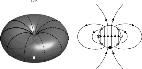
Sketches of the proposed current system, from Southwood & Kivelson (2007). The left-hand figure shows a dipolar shell of field lines at L = 15R_S on which currents flow between the Northern and Southern ionospheres. The thickness of the lines represents the magnitude of the interhemispheric current, while the solid and dashed lines indicate north–south and south–north currents, respectively. The right-hand figure is a sketch of the approximate magnetic field distribution produced by these currents in the equatorial plane. In practice, this would not be perfectly uniform as shown in the figure. The white dot on the left figure and the black dot on the right figure represent the same location on the L = 15 shell.

Open in new tabDownload slide

In this study, we shall investigate whether asymmetries in the upper atmosphere could plausibly generate such a system of currents. In Section 2, we describe a model of the thermosphere–ionosphere and the temperatures and winds it predicts when forced with asymmetric heating. Sections 3 and 4 describe the resulting current systems and magnetic perturbations; Section 5 discusses the plausibility and consequences of our results.

2 THERMOSPHERE–IONOSPHERE MODEL

2.1 Details of the model

Our thermosphere–ionosphere model is a global circulation model, essentially identical to that used by Smith et al. (2007) and Smith & Aylward (2008). Here we briefly describe the nature of the model and the modifications that have been made to it to suit this study.

2.1.1 Outline of the model

The thermospheric model used by Smith et al. (2007) and Smith & Aylward (2008) was a two-dimensional version, in latitude and altitude, of the three-dimensional model described by Müller-Wodarg et al. (2006). In the former model, longitudinal symmetry was assumed in order to study the rotational coupling of the thermosphere–ionosphere and magnetosphere in detail. For this study, we are specifically interested in longitudinal asymmetry, so we move back to a three-dimensional model. This is a trivial step because the full three-dimensional equations are already represented in the code, as described in detail by Müller-Wodarg et al. (2006). Briefly, the model solves the Navier–Stokes equation on a fixed latitude–longitude–pressure grid, including terms due to advection, curvature, Coriolis forces, viscosity, pressure gradients and ion drag. Neutral temperatures are calculated taking into account advection, viscous heating, Joule heating, thermal conduction and adiabatic heating and cooling, in addition to the arbitrary heating distributions described below.

We do not explicitly calculate plasma flows either in the ionosphere or in the magnetosphere. We assume a simple, fixed axisymmetric plasma flow distribution for the magnetosphere, as described below, sufficient to drive a reasonably realistic baseline distribution of Joule heating and ion drag in the thermosphere. The electric fields associated with these plasma flows are assumed to penetrate unmodified across the full depth of the region that we model. Our calculations of perturbations to the magnetosphere are then based entirely on considerations of current closure and application of the Biot–Savart law. We do not at this stage attempt to model how the currents that we predict may feed back on the dynamics of the magnetosphere.

2.1.2 Resolution of the model

The increase in dimensionality of our model compared to that used by Smith et al. (2007) and Smith & Aylward (2008) necessitates a decrease in resolution in order to maintain manageable run times. For this study, we use a latitude resolution of 2°, a longitude resolution of 10° and 20 pressure levels at a resolution of 0.5 scale heights. The grey lines in Fig. 2 show how the 2° latitude resolution maps to the equatorial magnetosphere along dipole field lines. The base of the model is at a pressure of 100 nb, with the base temperature held at 143 K consistent with the temperature profile presented by Moses et al. (2000). All runs presented here start ‘cold’ at a global temperature of 143 K and are run forward for 400 planetary rotations. This run time is sufficient for the model to reach approximate thermal and dynamical equilibrium (Smith et al. 2005).

Figure 2

Mapping between the ionosphere and magnetosphere using dipole magnetic fields. The solid black lines show the latitude range of our heating distribution. The dotted lines show the approximate 12–15 L-shell range for the cam currents defined by Southwood & Kivelson (2007). The dashed line shows the location of the flow shear in our simplified model of rotational flow in the magnetosphere, coinciding with the main auroral oval in the interpretation of Cowley et al. (2004). The thin grey lines (two of which lie contiguous with the solid black lines already described) show how the latitude points of our thermosphere model map to the equatorial magnetosphere.

Open in new tabDownload slide

2.1.3 Global heating

The thermal structure of Saturn's upper atmosphere is not fully explained. The observed exosphere temperature of ∼400 K (Smith et al. 1983) is higher than can be explained by absorption of solar radiation alone. We are not specifically interested in this question here, but do wish to represent the thermospheric structure with a reasonable level of accuracy. We therefore artificially reproduce the observed exosphere temperature with an arbitrary and globally uniform heat source. This is similar to the approach taken by Müller-Wodarg et al. (2006) to reproduce the ∼400 K exosphere temperature using an arbitrary global distribution of ‘wave heating’. Our approach is to use the same form of vertical heating distribution as Smith et al. (2005):

1

where q_m is the heating rate per unit mass in W kg⁻¹, q_m∞ is the limiting value at the top of the thermosphere and p₀ is the characteristic pressure that determines the peak heating rate per unit volume. By trial and error, we choose parameters of q_m∞ = 1.6 W kg⁻¹ and p₀ = 4 nb to produce a reasonable match to the occultation data of Smith et al. (1983) and Hubbard et al. (1997), the former being represented by the temperature profile constructed by Moses et al. (2000). The resulting global temperature profile after 400 planetary rotations is shown in Fig. 3. Also shown is the heating profile, plotted in units of ⁠.

Figure 3

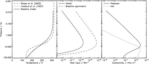
Left-hand panel: baseline global temperature profile (solid line) compared to the profiles presented by Hubbard et al. (1997) (dotted line) and Moses et al. (2000) (dashed line). The thermospheric part of the Moses profile is based on the data of Smith et al. (1983). Middle panel: heating profiles per unit volume for the baseline temperature profile in the left-hand panel. Solid line: global baseline heating rate; dashed line: asymmetric heating rate imposed across a limited longitude–latitude range (see text). Right-hand panel: conductivity profiles in mho m⁻¹ for the baseline temperature profile in the left-hand panel. Solid line: Pedersen conductivity; dotted line: Hall conductivity.

Open in new tabDownload slide

Note that, in principle, we could derive a vertical profile of heating and cooling that exactly matched any temperature profile. However, we think it preferable to use a simple analytic heating profile that produces temperatures approximately matching the observations.

2.1.4 Asymmetric heating

In addition to this global heating distribution, we introduce an asymmetric heating distribution. Some possible sources of such asymmetric heating of the thermosphere have been discussed previously by Smith (2006) and will be discussed further in Section 5. However, at this stage we shall not dwell too much on the possible origin of this asymmetric heating – we are principally interested in the hypothetical effects of such a heat source if it does exist.

We choose to impose the heating using the same functional form of heating distribution described above (equation 1), but within a limited latitude and longitude range. For our standard run, we add an extra component of heating with q_m∞ = 50 W kg⁻¹ and p₀ = 4 nb (see Fig. 3) in the longitude range 180°–360° and the latitude range 72°N–78°N. Within this region the asymmetric heating therefore has the effect of increasing the existing heating by a factor of ∼30 while not changing its dependence on pressure.

The broad longitude range chosen reflects the simplest possible form of longitudinal asymmetry. This distribution in longitude is equivalent to a square wave plus a constant, and thus contains a combination of odd harmonics m = 1, 3, 5 … and a zero-frequency harmonic. The heating is imposed only in the Northern hemisphere in order to be certain that a hemispheric asymmetry is introduced. Fig. 2 shows how the latitude range of the asymmetric heating maps into the magnetosphere in a dipole field.

The specific latitude range 72°N–78°N is chosen because this introduces the heating in a region coupled to the field lines that are expected to carry the cam currents. Using a dipolar model, the range 12–15R_S in the magnetosphere maps to latitudes of 73.2°N–75°N. Thus, our heating completely encapsulates this range. Furthermore, as described below, we choose the latitude 75° as the approximate boundary between corotational and subcorotational flow in our simplified magnetospheric plasma flow model. Thus, a second reason for the location of our asymmetric heating, and the reason for the specific latitude limits of 72° and 78°, is that it is centred on this important latitude for thermospheric dynamics.

2.1.5 Ionosphere

Thermosphere–ionosphere coupling is implemented using the same simplified scheme described by Smith & Aylward (2008). This entails using data from an ionosphere model to produce a global fixed map of Pedersen and Hall conductivities and then fixing these in such a way that the height-integrated conductivities are independent of variations in the thermal structure. We wish to keep our model as simple as possible, so use a globally averaged profile of conductivities at all latitudes and longitudes. We generate this by taking equinox ionosphere profiles at 70°N and 70°S from a recent version of the Moore et al. (2004) ionosphere model (Luke Moore, private communication). We average these in longitude, producing average ionospheres for mid-to-high latitudes in both the Northern and Southern hemispheres, and then average these two profiles to produce a single representative ionosphere. We then calculate a profile of conductivity, which we fix according to the procedure described by Smith & Aylward (2008). We choose to use ionosphere profiles from a latitude of 70° to provide a reasonable representation of conductivities across the mid-to-high latitude range in which we are interested.

The resulting profiles of conductivities calculated for our baseline thermal structure are shown in Fig. 3. This shows that across most of our altitude range Pedersen conductivity is much more important than Hall conductivity, although Hall conductivity is more important at the base of the model and may make a dominant contribution to currents at altitudes that we do not study here. Across our altitude range, the height-integrated Pedersen and Hall conductivities are 0.76 and 0.55 mho, respectively.

2.1.6 Rotational coupling to the magnetosphere

Smith & Aylward (2008) presented a detailed analysis of the interaction between the thermosphere–ionosphere and magnetosphere at flow shears in the rotational profile of the magnetosphere, as represented by the model of Cowley, Bunce & O'Rourke (2004). Such an analysis is not the purpose of this study, nor is it possible with the reduced latitudinal resolution necessitated by the use of a three-dimensional model. We therefore use a very simplified model of the rotational plasma flows in the magnetosphere, which is enough to represent the overall forcing of the thermosphere–ionosphere by the magnetosphere without introducing unnecessary complications. To this end we assume that the plasma in the magnetosphere rigidly corotates with the planetary angular velocity (which, for the purposes of the thermosphere model, means rigid corotation with the lower boundary pressure surface) at colatitudes greater than 15°. Polewards of this colatitude we assume 30 per cent of rigid corotation. The location that this colatitude maps to in a dipole magnetic field is shown in Fig. 2 by the dashed line.

These plasma flows then interact with the thermosphere using the same formulations of Joule heating and ion drag described by Smith & Aylward (2008). We assume a constant vertical magnetic field at all latitudes, taking a round value of 60 000 nT consistent with the fields observed in Saturn's polar regions. The advantage of assuming a vertical field is transparency in linking field-aligned currents to the thermosphere model, since individual field lines can be correlated uniquely with latitude–longitude grid points. The advantage of assuming a constant field is that our model of conductivity can be held fixed at all latitudes while retaining a reasonable degree of self-consistency. Both assumptions are good at high latitudes but become progressively weaker moving towards the equator. At latitudes below about 60° at which the assumptions begin to become genuinely poor, our calculations are unlikely to make an important contribution to the cam currents, since these regions map to radii of less than ∼4R_S.

2.2 Results

We now describe the results of one run encapsulating all of the elements described above.

The overall behaviour of the neutral winds is essentially identical to that described by Smith et al. (2007), showing a high degree of axial symmetry. Ion drag generates a region of subcorotating neutral flow at high latitudes, which is forced by Coriolis forces into a convergent polewards flow that generates heating at the pole itself. This behaviour has already been comprehensively analysed by Smith et al. (2007) and Smith & Aylward (2008). Instead, we focus here on the axially asymmetric behaviour that is induced by the axially asymmetric component of heating.

The asymmetric components of the temperatures and horizontal winds are shown in Fig. 4 for the pressure level n = 6 (at a pressure of ∼8 nbar). This altitude coincides with the peak of the Pedersen conductivity and therefore makes the greatest contribution to coupling with the magnetosphere. The asymmetric components are calculated by longitude averaging each quantity and then subtracting this average from the original value at each point. It is perhaps not surprising that the asymmetric heating has introduced an asymmetry in the temperatures and winds! What is interesting about these results is that the very simple and geometrically confined heat source has produced a globally smooth and symmetric distribution of temperatures and winds, which very nearly varies sinusoidally in longitude.

Figure 4

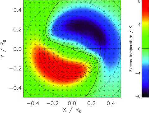
Excess temperature and winds at pressure level n = 6 in the northern polar region after the axially symmetric values have been subtracted. The plot is shown using an orthographic projection, equivalent to viewing the planet from infinity. The colour-scale indicates the excess temperature, with zero excess temperature indicated by the solid contour. The arrows show the size and direction of the excess horizontal wind. The length of the arrows represents the total size of the excess horizontal wind: the longest arrows show a speed of ∼20 m s⁻¹. The dotted lines show circles of constant latitude at 10° spacing; the dot–dashed line represents our zero longitude; the dashed circles show the latitudes mapping to ∼12–15R_S in the magnetosphere; and the triple dot–dashed contour shows the region in which our asymmetric heat source is applied.

Open in new tabDownload slide

To illustrate this, we have Fourier decomposed the longitudinal distribution of temperatures and winds at each latitude. The upper panels of Fig. 5 show the relative amplitudes of the first five harmonics as a function of latitude for the temperature, meridional wind and zonal wind. The thick lines show the equivalent decomposition of the square wave heating distribution. With the exception of the meridional winds in the range 65°N–75°N, the higher order harmonics are everywhere relatively less significant than they are in the heating distribution. Thus, the higher order harmonics in the heating distribution have been very effectively ‘washed out’ by the thermospheric winds to produce a smoothly varying and nearly sinusoidal pattern of thermospheric flow. It is also notable that the odd harmonics (m = 3, 5) are both more significant than the next lowest order even harmonics (m = 2, 4), suggesting that most of the asymmetric structure does indeed originate from the heating distribution, which contains only odd harmonics. The lower panels in the figure will be discussed later.

Figure 5

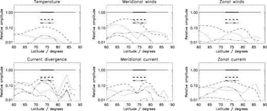
Fourier decomposition of temperature and winds (at the n = 6 pressure level) and current parameters (height-integrated). The solid, dotted, dashed, dot–dashed and triple dot–dashed lines, respectively, show the relative amplitude of the m = 1, 2, 3, 4 and 5 harmonics of the longitudinal distribution of each parameter as a function of latitude. The thick lines show the equivalent information for the square wave heating distribution (which by definition does not contain any even harmonics).

Open in new tabDownload slide

We do not show equivalent plots to Figs 4 and 5 for the Southern hemisphere, because the asymmetries are negligible, that is, the asymmetry introduced by heating in the Northern hemisphere does not significantly propagate across the equatorial thermosphere. This opens up the possibility that two independent asymmetric heat sources could exist in each hemisphere, driving rotating signatures in the magnetosphere at different rates (see Section 5).

3 INTERHEMISPHERIC CURRENTS

3.1 Calculation of currents

Given the distribution of winds, plasma flows, conductivities and magnetic fields discussed above, we calculate the distribution of horizontal currents in the thermosphere–ionosphere using the same procedure as Smith & Aylward (2008). Inevitably there are regions where these currents are convergent or divergent, and in these circumstances we require that the current is somehow closed. This can occur either by the local generation of an electric field that drives currents opposite to the wind-driven currents or by the current flowing along field lines into the magnetosphere, where the current can complete the circuit either by flowing across field lines in the magnetosphere or by flowing across a conductance in a connected region of the thermosphere–ionosphere. We assume here that none of our current closure is provided by cross-field line currents in the magnetosphere; all current closure occurs in the thermosphere–ionosphere.

Since we require our current systems to be quasi-static, we would expect any induced electric field to be slowly varying and thus to persist for long enough to penetrate along the magnetic field lines to the opposite hemisphere. Hence, any closure current driven in the ionosphere must flow in both hemispheres. Fig. 6 shows the situation as an equivalent circuit diagram. The winds in both the Northern and Southern hemispheres act effectively as current sources providing currents I_N and I_S, which must close through the conductances Σ in the Northern and Southern hemispheres (which in this study are assumed to be equal). These conductances are connected in parallel by ideal wires, representative of the magnetic field, which carry a current I_∥. An identical voltage V must be induced across both conductances and therefore an identical current I_C=ΣV must flow through each. Applying current closure at each junction, it is clear that I_C = 0.5 (I_N+I_S) and I_∥ = 0.5 (I_N−I_S). Half of the closure current for the north flows in the south, and vice versa, and since these currents must flow along the field in opposite directions, the net interhemispheric current must be half the difference between the current supplied by each hemisphere.

Figure 6

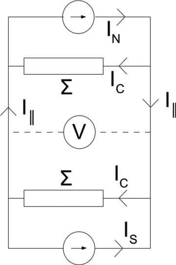
Sketch of an idealized interhemispheric circuit. The Northern and Southern hemispheres each contains both an ideal current source, representing the wind-generated currents, and a conductance. The vertical wires in the sketch represent the highly conducting magnetic field lines connecting the two hemispheres.

Open in new tabDownload slide

In reality, the current that is required to close is the divergence of the horizontal current in each hemisphere. Applying the model described above, it is clear that the current j_∥ flowing along the magnetic field between the hemispheres from north to south is

2

where J_N and J_S are the horizontal currents in the Northern and Southern hemispheres, respectively. The minus sign is introduced relative to the above discussion because a positive divergence in the Northern hemisphere implies a current flowing from south to north.

A secondary effect of the induced electric field is energy and momentum transfer between the hemispheres. In the thermosphere, this is manifested as Joule heating and ion drag. This has the potential to produce feedback effects, which may change the nature of the thermospheric flows. To analyse this we would need to explicitly calculate the induced electric fields: for this study, we simply assume that the interhemispheric current is given by the formula above and neglect interhemispheric energy and momentum flows.

3.2 Results

Fig. 7 shows the asymmetric horizontal currents in the Northern hemisphere and the asymmetric component of their divergence, in a similar format to Fig. 4. This figure shows only the divergences of the horizontal current in the northern polar region. There are also divergences in the Southern hemisphere, but these are negligible in comparison and are not shown. We ignore longitudinally symmetric divergences. Although these may be involved in currents flowing into the magnetosphere, they will by definition produce an identical signal at all longitudes, thus not contributing to the cam current system even if they are important in terms of global angular momentum transfer. However, it is worth noting that since we are imposing extra heating in the Northern hemisphere, we do observe a small north–south asymmetry in the longitudinally symmetric component of the current divergence.

Figure 7

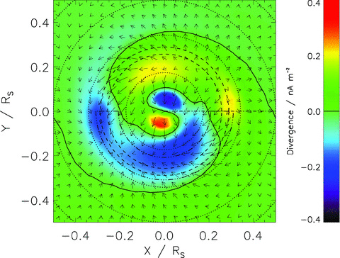
Horizontal currents and their divergences in the northern polar region. The colour-scale indicates the size of the divergence. Note that a positive divergence implies a downward current, corresponding to the south–north current in the equatorial plane. The solid line is a contour of zero divergence, and because the divergences in the Southern hemisphere are negligible, this is, to a very good approximation, magnetically connected to the equivalent solid line in Fig. 8. The arrows show the size and direction of the height-integrated Pedersen and Hall currents at each location. The longest arrow represents a current of ∼1 mA m⁻¹. The dashed, dotted, dot–dashed and triple dot–dashed lines have the same meaning as in Fig. 4.

Open in new tabDownload slide

There are two interesting features of the distribution of current divergence. First, the regions of positive and negative divergence show a clear spiral structure. This appears to be a consequence of the action of the Coriolis force on thermospheric winds, and will be discussed below. Secondly, a Fourier decomposition of the distribution of current divergence in longitude (Fig. 5) shows that the m = 3 and 5 harmonics are almost as significant in the distribution of current divergence as in the square wave heating distribution in the range 70°N–75°N. Since in our simple model of current closure the current divergence directly determines the interhemispheric current in the magnetosphere, we can therefore expect some higher order harmonics to be present in the resulting magnetic field perturbations. It is also worth noting that these higher order harmonics are much more pronounced in the current divergence than in the meridional and zonal horizontal currents. This is because taking the divergence increases the relative amplitude of the higher order harmonics. Thus, the situation that we predict in which the m = 1 harmonic is relatively dominant is only possible because the action of the thermosphere significantly reduces the relative amplitude of the higher order harmonics in the horizontal wind and current distributions before the divergence is calculated. This leads us to the general suggestion that the thermosphere promotes the formation of current systems with m = 1 symmetry by favouring this mode over higher order harmonics.

Fig. 8 shows the resulting field-aligned interhemispheric currents mapped into the equatorial plane of the magnetosphere. We use a dipole field for all calculations in this study as a sufficient approximation in the inner region of Saturn's magnetosphere. The greatest current densities shown are of the order of 0.1 pA m⁻² at L∼ 4, inside the region of the predicted cam currents. The size of the current then decreases rapidly with distance from the planet due to the inverse cube relationship of the magnetic flux density.

Figure 8

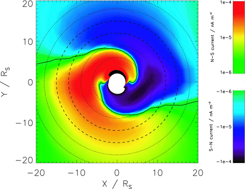
Interhemispheric currents mapped into the equatorial plane. The colour-scale indicates the size and direction of the interhemispheric currents. The solid line is a contour of zero interhemispheric current. The dashed lines show the L-shells 12 and 15 between which the current system proposed by Southwood & Kivelson (2007) is predicted to flow. These dashed lines are magnetically connected to the equivalent dashed lines in Fig. 7. The dotted lines shows L-shells at a spacing of 3R_S, thus indicating the locations of the five L-shell ranges used to produce Fig. 9.

Open in new tabDownload slide

4 MAGNETIC FIELD PERTURBATIONS

4.1 Calculations using the Biot–Savart law

To calculate the magnetic field perturbations, we treat the magnetic field lines as discrete wires carrying all of the current flowing out of each latitude–longitude cell in the atmosphere. Using the relatively low resolution of the thermosphere model, this produces poor results, so we linearly interpolate field-aligned currents on to cells of size in longitude and in latitude. Each magnetic field line originating at the centre of one of these cells is then divided into approximately 100 sections of equal length spanning the range from the ionosphere to the equatorial plane. Finally, we apply the Biot–Savart law to these sections, taking into account both hemispheres, to calculate the induced magnetic field in the equatorial plane.

4.2 Results

4.2.1 General morphology

Fig. 9 shows the calculated magnetic field perturbations in the equatorial plane. The first five panels show the magnetic field induced by the currents flowing in five adjacent L-shell ranges (6–9, 9–12, 12–15, 15–18, 18–21), and the final panel shows the total magnetic field induced by all of these contributions. The total size of the flux density is shown by the colour contours and the direction of the field is shown by the arrows. The dashed lines show the L-shell ranges used to calculate the field shown in each plot, and the solid line the orbit of the hypothetical spacecraft described below.

Figure 9

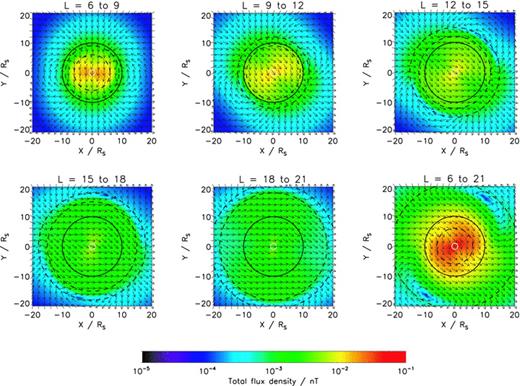
Magnetic field perturbations in the equatorial plane. The first five plots show the field perturbations due to currents flowing on specific ranges of L-values, as marked and indicated by the dashed lines; the final plot, at the bottom right-hand side, shows the total field perturbation due to currents flowing on magnetic shells in the range L = 6–21, again indicated by the dashed lines. The colour-scale indicates the magnitude of the flux density. The arrows indicate the direction of the perturbation field. The solid line on each plot indicates the orbit of the hypothetical spacecraft discussed in the text.

Open in new tabDownload slide

The magnetic fields induced by each L-shell range are similar in that they are all roughly uniform within the current-carrying shells, and roughly dipolar beyond them. This is a simple consequence of the asymmetry being dominated by a sinusoidal variation in longitude, and is essentially identical to the magnetic field that Southwood & Kivelson (2007) described, which would be induced by currents flowing along a narrow range of L-shells with this type of longitude asymmetry. More interesting than this is that the orientation of the roughly uniform field produced within each L-shell range is different, rotating eastward with increasing radial distance. The total magnetic field vectors in the final panel also show this rotation, although the behaviour is slightly more complex when different contributions are combined. This effect will be discussed further below.

The observation that the magnetic field induced by this whole range of L-shells is approximately uniform is enough to match the Southwood & Kivelson (2007) model. However, in order to emphasize this point, we show in Fig. 10 the magnetic field perturbations that would be observed by a spacecraft in a circular orbit at 10R_S. This shows that the observed radial and azimuthal fields are approximately out of phase by 90° and are a good match to a sinusoidal model, the azimuthal field appearing closer to a perfect sinusoid. While it is clear that the morphology of the magnetic field perturbations is a good match to the observations, the magnitude of the field is not. The typical fields observed by a spacecraft are of the order of a few nT, whereas our predicted fields are two orders of magnitude lower than this, of the order of 10 pT. Some possible mechanisms for increasing the magnitude of the field are discussed in Section 5.

Figure 10

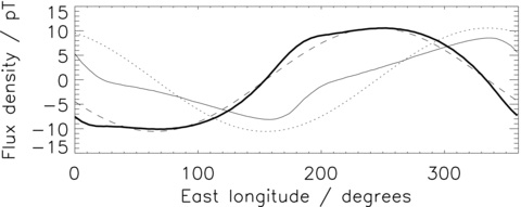
Magnetic fields perturbations observed by a spacecraft in orbit at radius 10R_S. The thick and thin solid lines show the azimuthal and radial fields, respectively. The dashed and dotted lines show two sinusoids, out of phase by 90° with their phase and amplitude adjusted by eye to fit the model output.

Open in new tabDownload slide

4.2.2 Phase variation with radial distance

Also of interest is the relative phase of the magnetic field perturbations at different radial distances. Gurnett et al. (2007) found that within ∼12R_S the phase of the magnetic field perturbations was almost independent of the distance, but that beyond this radius a large phase lag of ∼ 40° developed by ∼ 20R_S. In this context, ‘phase lag’ implies that the perturbation is shifted slightly westwards at larger radial distances as would be expected if the disturbance propagates outwards from a source in the inner magnetosphere.

In our results, we find that the opposite situation develops. As has already been commented, the field perturbations induced by different L-shell ranges shown in Fig. 9 rotate eastwards with increasing radial distance. As a result, the magnetic field perturbations at larger radial distances lead those at smaller radial distances. This is illustrated by Fig. 11, which shows the normalized azimuthal and radial fields predicted by our model at six radial distances. In both cases, there is a clear eastward phase shift with increasing radial distance. This phase shift is much clearer in the azimuthal field. Interestingly, the azimuthal field shows most of its phase shift beyond 6R_S, while the radial field shows very little variation beyond this radius.

Figure 11

Phase shifts of magnetic field perturbations with radial distance. The left- and right-hand plots, respectively, show the variation of the azimuthal and radial field perturbations with longitude for six L-values. The amplitude of each trace has been normalized. The dashed and dotted lines show a sinusoid fit to the data with a phase varying linearly with the L-value. The sinusoid fits for the azimuthal and radial fields have been determined independently. Note that this plot is similar to fig. S3 of Gurnett et al. (2007), but they use a west longitude system, such that a left-to-right shift on their figure represents the opposite phase shift to a left-to-right shift on our figure.

Open in new tabDownload slide

Fig. 11 also shows sinusoidal fits to the model output. We have fitted sinusoids by eye to the field perturbations at L = 3 and 18, and then interpolated the phase linearly between these two extremes. Based on these fits, the azimuthal and radial fields show phase shifts of 80° and 30°, respectively, across the range shown. At L = 3, the azimuthal field leads the radial field by 95°, while at L = 18, it leads by only 45°. However, it is clear that the sinusoid fit to the radial field is poor, so this inferred change in the phase relationship between the two components should not be considered significant. However, the difference in magnitude of the phase shifts for the two components is clear and significant and demands an explanation.

The phase shift itself occurs simply because the longitudinal variations of the currents flowing on each set of L-shells are not precisely in phase. This effect is almost certainly a consequence of the importance of Coriolis forces in the upper atmosphere. Any meridional transport will tend to be modified by Coriolis forces to produce zonal motions, such that features at adjacent latitudes are unlikely to be coupled without a longitudinal phase difference being generated by zonal wind shear. Specifically, an equatorward motion will be modified westwards and a poleward motion modified eastwards by Coriolis forces. The effects of this are visible in Figs 4, 7 and 8, all of which display clear spiral structures about the pole, oriented south-west to north-east at the planet. Although we are only presenting the results of one model run, we can thus tentatively suggest that phase shifts of this nature – but possibly not of this magnitude – should be expected to be a universal feature of cam currents driven by upper atmospheric winds.

The difference in the magnitude of the phase shifts in the azimuthal and radial components can be explained by analysing the distribution of magnetic field perturbations produced by a specific shell of field-lines. Here, we analyse the magnetic field perturbations produced by currents on L-shells in the range 12.5–13.5. We choose this range because it lies in the centre of the postulated region of cam currents, and the radial distance L = 13 maps almost exactly to a latitude of 74°, which coincides with a ring of grid points in the thermosphere model. This means that the currents flowing on this small range of shells are almost exclusively determined by the divergence of the currents flowing at this specific well-defined latitude. Fig. 12 shows a Fourier analysis of the amplitude of the first five harmonics of the longitudinal distribution of magnetic field perturbations produced by this range of shells, as a function of the radial distance. The line formats are the same as those in Fig. 5.

Figure 12

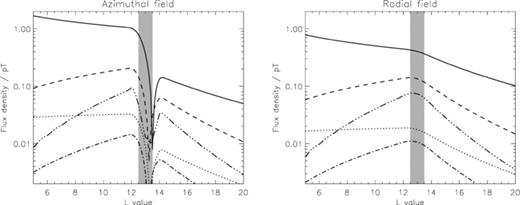
Fourier analysis of magnetic field perturbations due to currents flowing in the range L = 12.5–13.5R_S, shown by the grey shaded region on the plot. The lines show, using the same formats as Fig. 5, the magnitudes of the first five harmonics of the longitudinal distributions of azimuthal and radial field perturbations.

Open in new tabDownload slide

The difference between the magnitude of the radial and azimuthal field perturbations either side of the current sheet is striking. The amplitude of the azimuthal field perturbation rises by a factor of ∼5 on crossing the current sheet in the direction of the planet, and also changes sign (which is not shown in the figure) while the radial field remains approximately constant. Thus, as we move outwards through the magnetosphere, the contribution to the azimuthal field from each shell that we cross becomes abruptly both small and negative. Since the phase of the perturbation at any radial distance is a weighted combination of the phases of all of the contributions from different magnetic shells at different distances, the sudden removal of one of these components can significantly alter this combination and allow the phase of the azimuthal field to change significantly over a relatively short radial distance. By contrast, the radial field generated by each shell of field lines has a significant influence on the field at both larger and smaller radii, such that we would expect the radial field signature to vary more gradually and be a mixture of contributions from a broader range of radial distances.

The Fourier analysis also allows us to suggest why the azimuthal field is closer to a perfect sinusoid. As we have just described, most contributions to the azimuthal field are made inside a current-carrying shell. Fig. 12 clearly shows that inside a shell the m = 1 harmonic grows with decreasing radial distance, while the higher order harmonics all decline in amplitude. The same is true for the radial field inside a shell, but outside the shell the m = 2 and 3 harmonics in the radial field decline at a similar rate to the m = 1 harmonic. Since, as discussed above, a shell makes a significant contribution to the radial field at both smaller and larger radial distances, the latter effect means that higher order harmonics in the radial field produced by currents at a given radial distance can persist to much larger radial distances. This effect is apparent in Fig. 11, in which a single non-sinusoidal structure persists from L = 9 all the way out to L = 18.

5 DISCUSSION

5.1 Possible origin of heating

We have shown that asymmetric heating at high latitudes can generate magnetic field perturbations of the appropriate distribution in the magnetosphere. However, our imposed heating distribution was essentially arbitrary. We now suggest some possible origins of such a heating distribution. Two issues need to be addressed: the location of the rotating feature that ultimately drives the heating and the mechanism for generating the heating itself.

The key property of the feature that drives the heating is that it must rotate stably at a period close to that at which the magnetic field perturbations are observed to rotate. Since this period is close to the rotation period of the lower atmosphere as observed in the motion of cloud features, the heating must originate in a layer of the atmosphere that does not substantially subcorotate due to drag from the magnetosphere. This would appear to rule out the high-latitude thermosphere that is directly coupled to the subcorotating outer magnetosphere. However, it does not rule out regions at lower altitudes or latitudes. Therefore, our heat source could be located anywhere in the lower and middle atmosphere or at mid-latitudes in the thermosphere.

The existence of stable features rotating with the planet in the lower atmosphere is well established. Numerous relatively small storm systems are observed at Saturn, and the Great Red Spot of Jupiter has existed stably for over 150 yr (Ingersoll et al. 2004). Although these features are tropospheric, it is possible that such a large-scale vortex exists in the mid or high latitudes in Saturn's middle atmosphere, but has not been observed due to the relative difficulty in making observations of this part of the atmosphere. At Saturn, the persistence of the northern polar hexagon (first described by Godfrey 1988 and also a feature of the lower atmosphere) is now well established (e.g. Baines et al. 2009), and a similar or related feature in the middle atmosphere could also provide the asymmetry that we require.

It is quite clear that there is no evidence to support the existence of a comparable stable feature in the mid-latitude thermosphere. However, we can speculate that such a feature would be most likely to persist at regions of shear in the zonal flow where vortices might be formed by the Kelvin–Helmholtz instability. Such a flow shear exists at the boundary between the higher latitude regions subject to subcorotational ion drag from the outer magnetosphere and the lower latitude regions connected to the corotating inner magnetosphere. Smith & Aylward (2008) showed that these lower latitude regions actually tend to supercorotate slightly, because the ion drag acting on the higher latitudes induces a poleward flow that is spun up by Coriolis forces. There is thus a point in this flow shear that rotates at the correct planetary period, and a vortex forming in this region could thus have the appropriate properties. In our model, such a vortex would lie approximately in the 72°–78° latitude range in which we impose our asymmetric heat source. Another possibility is that asymmetric heating is driven not by a discrete feature but simply by variation in the degree of turbulence in different longitude sectors. A discrete ‘storm’ localized in longitude could generate such an asymmetry across a large range of longitudes if it had a turbulent wake.

Any of these possibilities essentially represent asymmetries in the winds in various different regions of the atmosphere. In our model, we have represented such an asymmetry by an increase in thermospheric heating, but in practice any form of asymmetry in thermospheric forcing will produce an asymmetry that is likely to generate a corresponding asymmetry in the magnetosphere. A lower or middle atmosphere feature could generate an asymmetry in thermospheric forcing, if there was substantial generation of gravity waves which may break in the thermosphere and generate asymmetric heating and/or drag. A feature existing directly in the thermosphere would represent the asymmetry itself and would also generate asymmetries in Joule heating and ion drag.

5.2 Magnitude of field perturbations

As already discussed, our results provide a good match to the observed morphology of the magnetic field perturbations, but not to their magnitude. For our mechanism to explain the observations, the magnitude of the currents generated must therefore be greater by a factor of ∼100. There are several possibilities for providing this increase.

Most obviously, any of the atmospheric parameters that directly contribute to the size of the current may have been underestimated. A greater intensity of heating seems likely to increase the magnitude of the currents, but a factor of 100 seems unlikely to be achieved without grossly overheating the thermosphere. Similarly, changing the altitude or vertical distribution of the asymmetric heat source seems unlikely to produce the required increase. More plausible is that the conductivities are underestimated. Our ionosphere model, based on that of Moore et al. (2004), does provide a reasonable match to the observed electron densities at Saturn. However, there may be localized zones of enhanced electron density. For example, we would except such enhancements at or close to the main auroral oval.

If all other things remain equal, we would require an enhancement of the conductance by a factor of 100 to provide a commensurate increase in the interhemispheric currents. However, the existence of a sharp latitudinal gradient in conductance would represent an independent mechanism for producing a divergence in the horizontal currents that has not been studied directly here, since the divergences that we have calculated have been a direct consequence of structures in the horizontal winds only. Hence, in this scenario, we may not need a factor of 100 enhancement to supply the required currents, a possibility that deserves further study.

Even if a conductivity enhancement has an associated sharp gradient, a latitudinally extended enhancement may not provide the required enhancement in current density because it will also lead to increased ion drag, thus slowing the winds that generate the currents. Hence, a latitudinally thin region of enhanced conductivity is probably ideal, providing a large divergence in the horizontal current density at its edges without significantly impeding the neutral flow that generates the currents in the first place. However, a further problem with this might be the formation of almost equal and opposite interhemispheric current sheets at the northern and southern boundaries of the conductivity enhancement. These would flow on closely nested magnetic shells, producing almost equal and opposite field perturbations that would essentially cancel each other out. It is clear that a detailed assessment of the effect of various plausible conductivity enhancements is required.

A further possibility is that the asymmetric currents required may be generated at lower altitudes. This study has investigated principally the Pedersen conducting region of the upper atmosphere. The winds generated by an asymmetry in the Hall conducting region, which lies largely below our model's lower boundary at 100 nb, may drive more significant currents into the magnetosphere. However, it is worth noting that there is a limit to the depth at which such an asymmetry could be coupled to the magnetosphere. The field-aligned conductivity decreases with increasing neutral density, such that sufficiently deep in the atmosphere any asymmetric structures will be electrically insulated from the magnetosphere, even if there is sufficient ionospheric density to generate large horizontal currents.

Finally, a limiting factor in the magnitude of the divergences predicted by our model is the spatial resolution of the thermospheric grid. The latitude resolution of 2° and longitude resolution of 10° both correspond to spatial distances of ∼2000 km at the latitudes that map to the cam currents. Structures in the upper atmosphere related to auroral processes are known to exist on scales smaller than this. For example, the width of the auroral oval is of the order of 300–600 km (Cowley et al. 2004), implying that spatial gradients in parameters, such as the ionospheric conductance and plasma flow speeds, must occur on a still smaller scale, perhaps 100 km or smaller, an order of magnitude below our spatial resolution. Divergences that develop over these scales are not resolved by our model. Thus, the lower spatial resolution of our thermosphere model may partially account for the small size of the calculated magnetic field perturbations. A related issue is that due to the mapping between the thermosphere and equatorial magnetosphere, the 2° resolution of the model maps to relatively low L-shell resolution in the magnetosphere across our region of interest, as clearly shown by the grey lines in Fig. 2. This means that the interhemispheric currents that we calculate are distributed smoothly over many R_S, while in reality they may flow in much more spatially confined sheets.

5.3 Hemispheric asymmetries

This study has focused on an asymmetry introduced in the Northern hemisphere. This choice is completely arbitrary. What would be the effect of adding an identical heat source in the Southern hemisphere at the same longitude? The opposite sign of the Coriolis force in the Southern hemisphere would ensure that the winds generated are a mirror image of those in the north. The opposite sign of the magnetic field in the Southern hemisphere then further ensures that all divergences of horizontal currents would be identical, such that the currents driven by the two hemispheres would cancel each other out, producing zero interhemispheric current. However, it seems unlikely that two identical regions of heating could remain correlated in longitude in this way, unless there was an underlying driver much deeper in the planet.

Furthermore, recent research (Gurnett et al. 2009) has shown a hemispheric asymmetry in the rotation rates of radio emissions related to high-latitude magnetic field lines, with SKR emission from the Northern and Southern hemispheres exhibiting periods of about 10.8 and 10.6 h, respectively. If the same mechanism that generates the cam currents is also related to these radio emissions, then we would require two complementary regions of asymmetric heating in the north and south rotating at these two slightly different rates. Assuming that the perturbations in the Northern and Southern hemispheres were roughly identical in terms of the magnetic perturbations produced, and that they behaved essentially independently, we would expect them to beat against each other, sometimes interfering constructively and sometimes destructively, with a period of approximately 50 Saturn rotations.

Another simplification of our model is that the Northern and Southern hemispheres have identical ionospheric conductances, which would only be expected at equinox. We can predict the effect of seasonally variable ionospheric conductances if we reanalyse the equivalent circuit in Fig. 6 with independent northern and southern conductances Σ_N and Σ_S. If we assume to a first approximation that the thermospheric wind distributions are independent of the conductances, then the currents in the north and south will be proportional to these conductances, I_N=Σ_NV_N and I_S=Σ_SV_S, where V_N and V_S are effective wind-generated voltages in the Northern and Southern hemispheres, respectively. These modifications imply the following formula for the closure current I_∥:

3

As commented above, this implies that, if there are equivalent thermospheric asymmetries in the Northern and Southern hemispheres, the closure current will fall to zero. However, it also shows a symmetry in the dependence of the closure current on the northern and southern conductances. For example, the component of the closure current driven by V_N has exactly the same dependence on Σ_N as it has on Σ_S. This is due to two complementary effects. First, a larger Σ_N means that a larger current is generated by the winds in the Northern hemisphere, implying a commensurately larger closure current. Secondly, a larger Σ_S implies that a greater proportion of the closure current flows in the Southern hemisphere, also implying a larger interhemispheric closure current. The combination of these effects means that for fixed Σ_N or Σ_S, the above expression for I_∥ maximizes when the two conductances are equal.

A naive interpretation of this result implies that the interhemispheric current should maximize at equinox. However, the factors influencing conductance are complex, such that during solstice one conductance may rise much more than the other falls, making it difficult to predict how the interhemispheric current will change. Nevertheless, it is clear that if either of the conductances falls to a very small value during solstice (which seems perfectly possible with the correct combination of winter illumination conditions and ring shadowing), then the interhemispheric current will also fall almost to zero – either because very little current is being generated in the winter hemisphere or because very little current closes across the winter hemisphere.

All of these considerations make the assumption that solar insolation is the main driver of ionospheric conductance. While this seems highly likely at low latitudes, the exact balance between solar and auroral ionization at mid and high latitudes is open to question. If auroral ionization dominates at the latitudes where the cam currents are generated, then we might expect very little seasonal variation.

Finally, the above discussion assumed that thermospheric winds would remain independent of conductance. In practice, a larger conductance will increase ion drag and may therefore slow thermospheric winds and reduce the effective wind-generated voltages, producing a non-linear dependence of current on conductance. The effect of this would be to disrupt the hemispheric symmetry of equation (3). As commented above – and taking the example of currents generated by an asymmetry in the north – the two effects that produce the symmetry are that a rise in the conductance in the north will produce a proportionate rise in the generated currents and that a rise in the conductance in the south will produce a proportionate rise in the interhemispheric closure currents. If the winds that generate the currents are slowed by a rise in conductance in the north, the former effect would be slightly reduced. Thus, a larger conductance in the south would be most conducive to the existence of a large closure current generated by an asymmetry in the Northern thermosphere. So, in this scenario, we expect a northern asymmetry to produce the greatest effect during southern summer.

5.4 Radial phase shifts

As described in Section 4.2.2, we find that the phase of the magnetic field perturbations at larger radial distances leads those at smaller radial distances. This is a specific consequence of the action of the Coriolis force on structures in the thermosphere, and therefore the observation of such a phase shift would provide evidence of a thermospheric source for the cam currents. However, at present, there is clear evidence for a large radial phase lag, increasing with radial distance, beyond L∼ 12, and indications of a possible small phase lag, again increasing with radial distance, within this radius (Gurnett et al. 2007). The evidence for the phase lag in the inner region is marginal, and indeed Andrews et al. (2008) commented that the order of magnitude of this inner region phase lag was comparable to the scatter in their data. We thus choose to characterize the observed phase shift as undetermined within L∼ 12, and as almost certainly lagging beyond this radius.

Assuming that the Coriolis-driven phase lead is a universal feature of cam currents driven by the thermosphere, this significant phase lag at large radial distances would at present appear to rule out direct control of the magnetic field perturbations by the thermosphere beyond L∼ 12. However, within this radius, the possibility remains open. We can identify two scenarios in which the characteristics of the thermosphere-driven cam current system described here would be consistent with the observed phase shifts. First, the thermosphere-driven cam currents may be broadly distributed across the region within L∼ 12. In this case, we would expect our radial phase lead to be observable across this region. Secondly, the thermosphere-driven cam currents may be confined to a relatively narrow range of shells in the region of L∼ 12. This would be consistent with a sheet-like current system produced by a sharp latitudinal conductance gradient in the thermosphere, as discussed above. In this case, we would expect to see the radial phase lead only on the current-carrying shells themselves. Depending on the width of the current-carrying region, such phase leads might be difficult to detect with certainty.

5.5 Observational signature of heating

There is a possibility that the asymmetric temperature distribution that our model predicts may itself be detectable. The most likely probe of temperature variations in the upper atmosphere is infrared emission from the molecular ion. The infrared emissions from depend strongly on temperature, such that at an average temperature of 500 K, an increase (decrease) of 10 K roughly doubles (halves) the emission (Neale, Miller & Tennyson 1996). Our predicted temperature contrast is of this order of magnitude, so if it exists, it should be clearly present in the emissions. Current observations using a 4-m class telescope and moderate-resolution spectroscopy allow a measurement of temperature to an accuracy of ±20 K across the entire auroral region in ∼5 h. Using a 10-m class telescope could improve the signal to an accuracy of better than ±5 K on a similar time-scale. However, the maximum temperature contrast occurs in the subauroral region, just equatorwards of the auroral oval. In subauroral regions, the signal is much weaker than in the auroral region itself, with the equatorial signal only recently being detected after ∼20 h. Thus, an observation of the subauroral regions is unlikely to be allocated enough time to detect the predicted temperature variation (T. Stallard, private communication).

6 SUMMARY

We have studied the distributions of temperatures, winds and electrical currents driven in Saturn's upper atmosphere by a hypothetical asymmetric heat source in the thermosphere and subsequently examined the related magnetospheric current systems and field perturbations. Our principal conclusions are as follows:

• A square-wave distribution of heating is ‘washed out’ by thermospheric winds, such that the longitudinal distributions of temperature, winds and currents in the ionosphere are dominated by the m = 1 harmonic.

• If divergences in the resulting distribution of currents close via interhemispheric field-aligned currents, these produce magnetic field perturbations in the equatorial magnetosphere whose direction matches those predicted by the model of Southwood & Kivelson (2007).

• The size of these magnetic field perturbations are of the order of 10 pT, two orders of magnitude smaller than the observed magnetic field perturbations. This discrepancy may be explained by the low resolution of our model and/or an incomplete model of ionospheric conductance.

• The predicted magnetic field perturbations develop a phase lead with increasing radial distance. This is explained by the importance of the Coriolis force in the development of structures in the thermosphere. This phase lead is opposite to the phase lag that is observed (e.g Gurnett et al. 2007). This suggests either that thermospheric cam currents must flow only at smaller radial distances than those for which a phase lag is observed, or that they flow only on shells covering a very narrow range of radial distances.

This study clearly demonstrates the plausibility of a thermospheric driver for the rotating asymmetries in Saturn's magnetosphere. Further exploration of the many possible distributions of thermospheric forcing and ionospheric conductivity is required to determine whether this mechanism can reproduce the observations in full.

I would like to thank Nick Achilleos, Margaret Kivelson and Tom Stallard for useful discussions, and Luke Moore for providing the model ionospheres.

REFERENCES