Effects of cosmological model assumptions on galaxy redshift survey measurements Free

Abstract

1 INTRODUCTION

Galaxy redshift surveys will become an increasingly important source of cosmological information. The ongoing Sloan Digital Sky Survey III Baryon Oscillation Spectroscopic Survey (BOSS; Schlegel, White & Eisenstein 2009a) will measure redshifts for 1.5 million luminous red galaxies over 10 000 deg², providing cosmic variance limited constraints out to z∼ 0.6. The next generation of ground-based surveys, using multi-object spectrographs on 4-m class telescopes, will push this cosmic variance limit to z∼ 1.4 (e.g. BigBOSS; Schlegel et al. 2009b). In addition to pushing beyond these redshifts, the space-based experiments benefit from having no atmospheric contamination and a larger angular coverage compared to the ground-based surveys. The European Space Agency (ESA) Euclid mission (Cimatti et al. 2008; Laureijs et al. 2009), currently in the definition phase, will be able to measure redshifts for galaxies out to z∼ 2, thus measuring large-scale structure for the full range of redshifts over which dark energy dominates, according to standard models. Given the precision that these surveys will achieve, it is interesting to consider exactly how the measurements from these surveys can be used to measure the parameters of different cosmological models.

Galaxies are biased tracers of the underlying matter density field, in that they do not form a Poisson sampling of the matter distribution. On small scales, the number and distribution within each host dark matter halo are dependent on the non-linear behaviour of collapsed objects. On larger scales, the dark matter haloes that host galaxies can themselves be biased with respect to the matter distribution. However, on very large scales (k∼ 0.1 h Mpc⁻¹), the ratio between galaxy and matter power spectra is scale-independent and the galaxy distribution can be assumed to be a fair sample of matter overdensities (see e.g. Kaiser 1984; Rees 1985; Cole & Kaiser 1989). While modelling the full link between the galaxy and matter clustering is complicated, it is possible to use simple fits and models to extend the range of scales where the two power spectra can be easily linked. Although such bias modelling will be important for future surveys, the accuracy with which errors can be forecast does not depend strongly on the exact form of these models and we therefore assume a scale-independent bias in the rest of this paper. For similar reasons, we assume a linear power spectrum, ignoring scale-dependent growth in the clustering of the matter distribution.

Given the complications of galaxy bias, future cosmic microwave background (CMB) data (The Planck Collaboration 2006) will render the cosmological information available from the large-scale shape of the galaxy power spectrum or correlation function (Percival et al. 2002; Cole et al. 2005; Tegmark et al. 2006; Percival et al. 2007; Reid et al. 2010) less interesting than at present. Instead, analyses will focus on using the galaxy distribution as a standard ruler to measure the expansion of the Universe, and use the anisotropy and amplitude of clustering to measure the growth of structure within it (Guzzo et al. 2008; Wang 2008).

Following the cosmological principle, the galaxy distribution is expected to be statistically homogeneous and isotropic and measured correlation functions and power spectra should be spherically symmetric in real space. In practice, this symmetry is broken: redshift-space distortions (RSDs) are present because the measured redshift of a galaxy not only is caused by the Hubble expansion but also has a contribution from the comoving peculiar velocity of each galaxy with respect to the Hubble flow. Since the peculiar velocities of individual galaxies depend on the overdensity field, the resulting clustering signal will be angle dependent (Kaiser 1987). RSDs have been measured using both correlation functions and power spectra (e.g. Hawkins et al. 2003; Percival et al. 2004; Zehavi et al. 2005; Guzzo et al. 2008; Cabré & Gaztañaga 2009).

When we use the galaxy distribution as a standard ruler, we have to model not only the distance to the galaxies but also the rate at which distance changes with redshift: if we match surveys of small regions of the Universe at different redshifts, then we need to match both the angular size (related to the distances to the regions) and the depths of the regions. If we get the ratio of these two projection effects wrong, we see an anisotropic clustering pattern, which is called the Alcock–Palczynski (AP) effect (Alcock & Paczynski 1979). This effect is partially degenerate with the RSD (Ballinger, Peacock & Heavens 1996; Simpson & Peacock 2010). For a standard ruler that is small relative to the scales over which cosmological expansion becomes important, we need the angular diameter distance R_A(z) to project each part of the survey to the correct distance, and the derivative of the radial distance dr(z)/ dz≡R_r(z) to give each segment the correct depth (Blake & Glazebrook 2003; Hu & Haiman 2003; Seo & Eisenstein 2003; Hu & Haiman 2003).

Because measurements of geometry and RSD are correlated, the cosmological parameter measurements will also be correlated. The choice of cosmological model to test, which acts as a prior on the measurements, also acts to correlate the measured parameters. In fact, as we show in this paper, these two effects are strongly coupled: the importance of the measurement correlation depends on the model to be tested. Consequently it is important when making predictions for future surveys to clearly set out the cosmological model selection. For example, RSDs are often parametrized by bσ₈ and fσ₈, where b is the bias, σ₈ is the rms amplitude of fluctuations in the matter field in spheres of radius 8 h⁻¹ Mpc and f≡ d log G/ d log a, where G is the linear growth function (e.g. White, Song & Percival 2008; Simpson & Peacock 2010).1 In fact, this dependence follows from certain assumptions about the Universe, which also affect the geometrical constraints (see Section 3). It is therefore unphysical to make assumptions for one measurement but not for the other. In this paper, we consider how the choice of model affects the coupling between geometrical constraints and RSDs, moving from simple assumptions about the Universe to specific parametrizations of different models.

In order to demonstrate these effects we predict measurements that could result from a possible survey configuration undertaken by the Euclid satellite. We use the baseline parameters for this survey considered by the Euclid Assessment Team, which we briefly describe in Section 2. In Section 3, we review the measurements that can be made from galaxy surveys, and the Fisher matrix formalism by which predictions are usually made for galaxy surveys is introduced in Section 3.3. Section 4 discusses the models and how they affect the power spectrum. We show how the choice of model strongly affects predictions in Section 5. We discuss our results and conclude in Section 7.

2 THE Euclid GALAXY REDSHIFT SURVEY

In order to consider the (often hidden) effect of the cosmological model assumption on AP and RSD measurements, we consider the baseline Euclid spectroscopic galaxy survey as outlined in the Euclid Assessment Study Report (Laureijs et al. 2009). Euclid is a proposed mission to study dark energy through an imaging survey of galaxy shapes, exploiting galaxy weak lensing and a spectroscopic survey of galaxy redshifts exploiting the Baryon Acoustic Oscillations (BAO) technique for measuring cosmological evolution. In this paper, we only consider the cosmological information available from the spectroscopic component of the mission. Euclid is currently in the definition phase with possible launch date of 2017. While these parameters can be treated as the representative for a possible survey that could be provided by the Euclid experiment, the baseline is expected to evolve as the definition phase progresses and consequently these numbers may not match the final survey achievable by this experiment.

We assume that Euclid will provide a galaxy redshift survey over a 20 000 deg² sky area and will measure redshifts for emission line galaxies over the redshift range 0.5 < z < 2.0 with the precision of σ_z = 0.001(1 +z). The number density of galaxies follows the assumption that we can obtain redshifts for 50 per cent of galaxies with Hα emission stronger than 4 × 10⁻¹⁶ erg s⁻¹ cm⁻², following the number density distribution described in Geach et al. (2010). These galaxies are biased tracers of the mass distribution, and we adopt the redshift-dependent bias relations of Orsi et al. (2010). We fit to the power spectrum over wavenumbers k < 0.2 h Mpc⁻¹ for bins with z > 1.1. For 0.5 < z < 1.1, we cut this maximum scale approximately linearly to only fit to scales k < 0.15 h Mpc⁻¹ at z = 0.5 to match the increasing scale of non-linear structure at low redshift (Franzetti et al., in preparation). The relative importance of different survey parameters to the ability of constrain cosmological models parameters will be studied in Wang et al. (2010).

3 COSMOLOGICAL MEASUREMENTS FROM GALAXY SURVEYS

In this paper, we will only consider cosmological measurements resulting from using RSD and from using galaxy clustering as a standard ruler. We do not consider additional constraints from the relative clustering amplitude on small and large scales.

3.1 Redshift-space distortions

If the galaxy separation is small compared with the distance to the galaxies, overdensities and velocities are small, the galaxy velocity field is irrotational and the continuity equation holds, then we can write the redshift-space overdensity as δ^s_g(k) =δ_g(k) −μ²θ(k), where θ≡∇·u is the divergence of the velocity field and μ is the cosine of the angle between wavevector and the line of sight (Kaiser 1987; Hamilton 1997; Scoccimarro 2004). In this case, the redshift-space power spectrum P^s_gg(k) consists of three components

1

where a subscript ‘g’ refers to the galaxies and a subscript θ refers to the velocity divergence. The power spectra can be directly related if we can assume that the linearized Euler, continuity and Poisson equations hold in a perturbed Friedman–Robertson–Walker (FRW) universe, and we can write

2

where f≡ d ln G/ d ln a is the logarithmic derivative of the linear growth factor G. The linearized relationship between velocity divergence field and the matter overdensity field follows from the continuity equation and does not depend on the cosmological model or theory of gravity, although the numerical value of f will depends on the gravity model. If the background metric is different from FRW, this relationship might not hold. Assuming that equation (2) holds, the three power spectra have the same shape and there are now only two free parameters, which can be chosen to be bσ₈ and fσ₈, giving the amplitudes (rms in spheres of radius 8 h⁻¹ Mpc) of the real-space galaxy overdensity field and velocity divergence field.

We therefore see that, in order to write the RSD dependency in terms of bσ₈ and fσ₈, we already had to assume that the Universe follows an FRW model. Using f and b as parameters, the measured redshift-space galaxy–galaxy power spectrum is traditionally related to the real-space matter power spectrum through

3

Hereafter, for simplicity and without loss of generality, we drop σ₈ from the RSD parameters, although it should be remembered that the constraints are dependent on the amplitude of the matter overdensity field. If we drop the assumption of an FRW model, then we can still try to constrain these parameters, but equation (3) no longer holds. Equation (3) also assumes that we know the cosmological geometry in order to estimate galaxy separations. Obviously we cannot make this assumption as we wish to measure both the RSD and the cosmological geometry from the measured power spectrum.

In all subsequent computations, we will use linear Kaiser formula of equation (3) to model RSD on large scales and we will also assume that bias is not a function of k. Numerical simulations show that both these assumptions are approximations even on very large scales; linear RSD theory does not agree with simulations (see e.g. Scoccimarro 2004; Jennings, Baugh & Pascoli 2010) and galaxy bias displays scale dependence (see e.g. Angulo, Baugh & Lacey 2007) even on the scales of k∼ 0.1 h Mpc⁻¹. When analysing real data the non-linear effects in RSD and bias must be included: using equation (3) instead of a more accurate scale-dependent model would bias the estimates of cosmological parameters. We presume, however, that using the linear theory as given by equation (3) still gives accurate estimate of the Fisher matrix for the galaxy survey. This should be true as long as the real non-linear power spectrum is not significantly different from a linear one over the range of scales included in this work.

3.2 Geometrical constraints

We only consider galaxy clustering on radial scales that are sufficiently small that there is negligible cosmological evolution across them. In this case, an angular standard ruler measures R_A(z)/s, and a radial standard ruler measures R_r(z)/s, where R_A(z) is the (comoving) angular diameter distance, R_r(z) is the derivative of the radial distance and s is the scale of the ruler. For BAO, this scale corresponds to the comoving sound horizon at the baryon drag epoch. If, on the other hand, we use the full correlation function or power spectrum as our ruler, this corresponds to the average scale of the features. Forcing the observed ruler to be the same size in radial and angular directions gives the Alcock–Paczynski test (Alcock & Paczynski 1979). In order to simplify the equations we drop the explicit dependence on s and consider that the geometry only depends on R_A and R_r: it is worth remembering that errors presented for these parameters are actually errors on R_A/s and R_r/s. The ruler scale s depends on the cosmological model parameters. We assume that the parameters required will be constrained by future CMB experiments with an uncertainty that is far smaller than could be obtained from the galaxy survey observations. Consequently, this dependency does not affect the geometrical constraints that are recovered from the galaxy survey analysis, and we assume that s is known perfectly.

To analyse galaxy clustering data, we have to adopt a fiducial cosmological model. The angular and radial distances in our fiducial model will be different from real distances by the factors and ⁠, where quantities without a hat are computed in a fiducial model and hat denotes real value.2 The measured components of the wavenumber along and across the line of sight will also be different from the real ones by the same factor. The power spectrum in equation (3) will acquire additional angular dependence through the AP effect and the final measured power spectrum will be

4

where μ=k_∥/k and A=α_∥/α_⊥ (for details see e.g. Ballinger et al. 1996; Simpson & Peacock 2010). The galaxy power spectrum is scaled by the additional factor ΔV=α⁻²_⊥α⁻¹_∥ because the reference cosmology under(over)estimates the survey volume by the factor of ΔV.

3.3 Survey Fisher matrix

For the most general cosmological model we consider, we model the power spectrum of galaxies by equation (4) and use the parameter set p^4N={f(z_i), b(z_i), α_∥(z_i), α_⊥(z_i)}, where 1 < i < N and N is the number of redshift slices. For simplicity we now drop the explicit dependence on z_i.

Logarithmic derivatives of equation (4) with respect to p^4N are given by

5

6

7

8

and the errors on radial and angular distances are related to the errors on α_∥ and α_⊥ simply by

9

10

Equations (5) and (6) are similar to equation (3) in White et al. (2008), which means that AP only changes the constraints on b and f through cross-correlation terms in the Fisher matrix, so that the errors marginalized over α_∥ and α_⊥ are altered from those of White et al. (2008), but (as expected) the unmarginalized errors are not. Equations (7) and (8) have three terms; the first term comes from the effect of AP on volume, the second term is the effect of AP on RSD and the third term is the angular dependence of isotropic power spectrum induced by AP.

Using derivatives in equations (5)–(8) we will compute a 4N dimensional Fisher matrix F^4N of cosmological parameters p^4N (for details see Appendix A). The inverse of F^4N gives an optimistic estimate of how well the cosmological parameters p^4N will be measured in spectroscopic surveys.

4 COSMOLOGICAL MODEL ASSUMPTIONS

For a survey divided into N redshift slices, which we assume to be independent, the inverse of the F^4N Fisher matrix gives the estimated covariance matrix of the 4N cosmological parameters p^4N = (f, b, α_∥, α_⊥). The only cosmological dependence of these error estimates is that θ∝δ on the scales being tested. This condition follows from FRW (see Section 3.1) but could also hold in other types of metric. The measurement of α_⊥ and α_∥ assumes that we know either the shape of the isotropic power spectrum or at least a position of some easily detectable feature in the power spectrum (e.g. position of the first baryon acoustic oscillation peak) from other observations. In few years time, the Planck mission will measure the linear matter power spectrum with very high accuracy, which will strongly anchor these geometrical constraints.

For any given cosmological model and theory of gravity, the rate of structure growth and the radial and angular distances at different redshifts are coupled and can be uniquely determined from a smaller number of basic physical parameters. The reduction in the number of parameters to be constrained obviously results in improved measurements. We will now consider how predictions from spectroscopic galaxy surveys improve as we tighten the cosmological model. The first and most basic assumption is that the Universe follows an FRW metric, which we have already shown is one of the conditions required to enable RSD to be parametrized in the standard way.

4.1 Friedman–Robertson–Walker metric

Functions R_A(z) and R_r(z) relate the coordinate angular distance and the redshift distance to the real physical distances at redshift z and, although not always expressible in a simple form, can be defined as such in any cosmological model and space–time. If, however, we assume that the Universe follows an FRW metric, the radial and angular geometrical constraints are coupled

11

12

where

13

c is the speed of light, H₀ is a Hubble constant and H(z) is a Hubble parameter which is different in every cosmological model.

In a space–time different from FRW (e.g. other Bianchi Type I spaces or Lemaître–Tolman–Bondi models), equations (11), (12) and the relationship between the two distances are in general different. Equations (11) and (12) show that if we assume FRW the measurements of H and D_A are coupled and provide constraints on curvature Ω_k.

The coupling is direct: given a set of measurements H(z_i) in FRW metric, the angular distance can be approximated as

14

where

15

is the error induced by replacing the integral with a finite sum and second derivative of the H⁻¹ is evaluated at some unknown point z* inside the interval. The ΔI_j terms approximate the error induced by estimating the integral by a finite sum using the ‘trapezoidal rule’.

After solving equation (14) with respect to H⁻¹(z_k), we can compute derivatives

16

17

18

where δ_i,j is a Kronecker delta function, in the limit Ω_k→ 0 and transform a 4N dimensional Fisher matrix F^4N into a 3N+1 dimensional Fisher matrix F^FRW of variables p^FRW={f, b, α_⊥, Ω_k}.

4.2 wCDM model of dark energy

Following Chevallier & Polarski (2001), the equation of state of time-varying dark energy is often parametrized as

19

In this model, the energy density of all matter components is

20

where

21

and Ω_m is relative energy density of non-relativistic matter.

Within the w cold dark matter (wCDM) model the radial and angular distances at all redshifts are completely determined by five cosmological parameters w₀, w_a, Ω_m, Ω_k and h. Assuming wCDM in FRW space–time, but keeping f as an arbitrary function of redshift, the 4N dimensional Fisher matrix F^4N now becomes a 2N+5 Fisher matrix F^w on parameters p^w={f, b, w₀, w_a, Ω_m, Ω_k, h}. We will also consider an XCDM model which is a specific case of wCDM with w_a = 0.

4.3 ΛCDM model

Most cosmological data sets are consistent with a simple ‘standard’ cosmological model where dark energy is time-independent cosmological constant Λ. ΛCDM model is a specific case of wCDM with w₀=−1 and w_a = 0. In ΛCDM,

22

and angular and radial distances can at any redshift can be computed from just three cosmological parameters h, Ω_m and Ω_k. For ΛCDM model, we transform F^4N into a 2N+3 dimensional Fisher matrix on cosmological parameters p^Λ={f, b, h, Ω_m, Ω_k} and estimate constraints on p^Λ.

4.4 γ parametrization of growth

In previous sections, we did not make any assumptions about the parameters f and kept them as N model-independent numbers. If we pick a specific cosmological model and theory of gravity, the N variables f(z) will not be independent and can be computed from a smaller number of basic cosmological parameters.

In most conventional cosmological models and theories of gravity, the proportionality constant between matter and velocity overdensities only depends strongly on Ω_m and can be approximated by

23

where E(z) is total energy density of all matter components normalized to H₀, but in modified theories of gravity is not necessarily equal to H(z)/H₀.

Treating γ as a free parameter to be fitted, f, H and D_A at all redshifts are functions of six parameters p^γw={γ, p^w} in wCDM and just four parameters p^γΛ={γ, p^Λ} in ΛCDM. The Fisher matrix F^4N can then be transformed into a Fisher matrix on p^γw and ⁠.

4.5 General relativity

For wCDM family of cosmological models equation (23) with

24

is found to be a very good approximation to the structure growth in GR (Wang & Steinhardt 1998; Linder 2005). For ΛCDM this gives γ = 0.55. If GR is the correct theory of gravity, then f, D_A and H at every redshift can be computed from just five parameters p^wGR={h, Ω_k, Ω_m, w₀, w_a} in wCDM and three parameters p^ΛGR={h, Ω_k, Ω_m} in ΛCDM.

5 EFFECTS OF MODEL ASSUMPTIONS ON CONSTRAINTS

We will use the Fisher matrix formalism discussed above, combined with sample parameters for a survey that could be delivered by the Euclid experiment, to investigate how derived cosmological constraints depend on the model assumption, combining both geometric and structure growth information. In all subsequent computations, we will assume a fiducial ΛCDM cosmology with parameters Ω_m = 0.25, Ω_b = 0.05, Ω_k = 0, σ₈ = 0.8 and n_s = 1.0.

5.1 The effect of the geometrical model on structure growth

Fig. 1 shows constraints on function f(z)σ₈(z) in different redshift bins for a Euclid survey for different assumptions about the model adopted for the background geometry of the Universe.

Figure 1

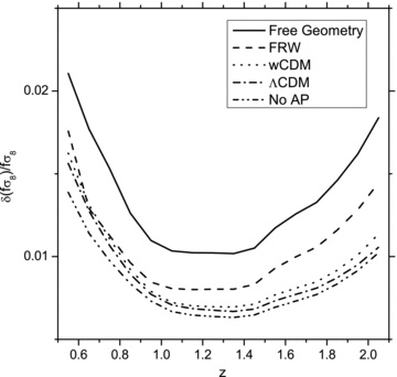
Constraints on fσ₈ in redshift bins of width Δz = 0.1 from the Euclid survey with different assumptions about background geometry of the Universe. The solid line, labelled as ‘Free Geometry’, shows constraints on fσ₈ when no assumptions are made about the background cosmology.

Open in new tabDownload slide

Solid line is derived without any assumptions about background cosmology other than the assumptions leading to equation (2) in Section 3.1. The predictions are encouraging. Even if no assumptions are made about background cosmology Euclid can measure growth with a precision better than 2.0%. Simply assuming FRW background brings the constraints down to 1.5 per cent. As expected, the constraints get better as we limit ourselves to models with a reduced number of basic parameters. Assuming wCDM or ΛCDM cosmologies further improves constraints on σ_f/f. If we used a fixed geometry when analysing RSD, the precision would be below 1 per cent at intermediate redshifts.

Fig. 1 clearly shows how big is the impact of assumptions about geometry on the measurements of growth. We see a significant improvement even if we only consider an FRW cosmology – similar to the assumption required to parametrize the RSD constraints. The constraints on f improve by a factor of more than 2 when we go from the most general case where we make no assumptions about background cosmology to the best case scenario where we assume that the geometry is known perfectly from other observations.

We see similar improvements if we parametrize growth using γ as in equation (23). Fig. 2 shows that the constraints improve significantly if we consider a ΛCDM model rather than the more general wCDM model. Adding Planck data would make the measurements even stronger and breaks the degeneracy between γ and h (for our treatment of Planck Fisher matrix, see Appendix B). With Euclid and Planck measurements combined γ can be measured to the precision of 7 per cent in wCDM and to the precision of 4 per cent in ΛCDM, while h can be measured to the precision of 2 per cent in wCDM and to the precision of 1.5 per cent in ΛCDM.

Figure 2

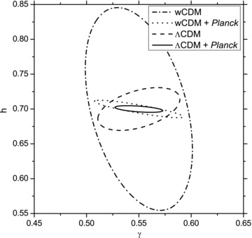
Constraints on parameters γ and h from the Euclid survey with different assumptions about background cosmological model.

Open in new tabDownload slide

5.2 The effect of structure growth assumptions on the geometrical model

Measurements of angular and radial distances at different redshifts are strongly affected by the assumptions about structure growth. Fig. 3 shows how the degeneracy with RSD affects the measurements of angular distance at different redshifts. The solid line is derived without assuming any specific theory for growth and treating f(z_i) as independent at different redshifts and from D_A(z) and H(z). If no constraints are placed on the form of the structure growth, then geometrical constraints are degraded by a factor of ∼4, compared to the case where structure growth is perfectly known. The simple assumption of an FRW metric proves extremely significant for our ability to measure D_A(z) at intermediate redshifts as it links the angular and radial distances through equation (14). Adopting this assumption almost removes the detrimental effect of having degeneracy with unknown RSD effects on the geometrical constraints.

Figure 3

Constraints on angular distance D_A as a function of redshift in redshift slices of width Δz = 0.1 for the Euclid survey with different assumptions about the growth of structure.

Open in new tabDownload slide

If we specify a cosmological model, the angular and radial distances at different redshifts can be expressed in terms of smaller sets of cosmological parameters. For the wCDM model of Section 4.2, Fig. 4 shows Fisher matrix predictions on the w₀, w_a correlated errors when other cosmological parameters are marginalized over. The constraints are extremely sensitive to the assumptions about the growth of structure. If we make no assumptions about the theory of gravity and allow the growth history to be completely free the resulting constraints are weak, giving roughly w₀∈ (−1.75, − 0.25) and w_a∈ (−2.17, 2.17) for marginalized errors at one σ confidence level. When we assume that the growth is parametrized by equation (23) the constraints are much stronger even when the γ parameter is allowed to vary. The γ parametrization results in w₀∈ (−1.45, − 0.55), w_a∈ (−1.25, 1.25) increasing the Figure of Merit (FoM) by about four times.3 Adding Planck priors to the Euclid measurements results in more powerful constraints on w₀ and w_a. Assuming GR w₀ is now constrained to be in the (−1.08, −0.92) interval and w_a is within (−0.13, 0.13) at one σ confidence level.

Figure 4

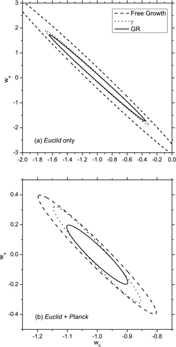
Constraints on cosmological parameters w₀ and w_a from the Euclid survey only and from joint Euclid and Planck analyses for different assumptions about structure growth. Coordinate axes on the top and bottom panels have different scales.

Open in new tabDownload slide

Other cosmological parameters of interest are Ω_m and Ω_k. Errors on their measurements will depend on whether we assume a time-dependent dark energy parametrized as in wCDM or time-independent cosmological constant Λ. They will also depend on the assumptions we make about growth. Fig. 5 shows constraints on Ω_m and Ω_k in wCDM and ΛCDM scenarios with three different models for growth history. Constraints on both parameters are extremely tight, for GR and ΛCDM the non-relativistic matter energy density is measured with a precision of about 1.4 per cent and the curvature is constrained to be less than 0.0013 from Euclid only.

Figure 5

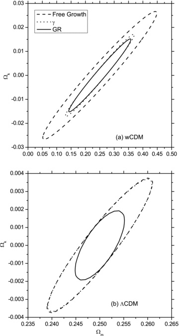
Constraints on cosmological parameters Ω_m and Ω_k in wCDM and ΛCDM models from the Euclid survey with different assumptions about the growth of structure. Coordinate axes on the top and bottom panels have different scales. The dashed and dotted lines cannot be distinguished by eye on the bottom panel.

Open in new tabDownload slide

6 TESTING DEVIATIONS FROM ΛCDM

The results presented in previous sections show that the estimates on cosmological parameters are very sensitive to the assumptions about the background geometry of the Universe and the growth of structure. In the most general case of free growth and unspecified geometry, the constraints on different parameters are weak because the RSD and AP effects are degenerate. As we make stronger assumptions about the cosmological model and theory of gravity, reducing number of independent parameters, the degeneracy between geometry and effects of structure growth reduces and the resulting constraints on cosmological parameters become tight.

Because of the reasons outlined above the best method to analyse the angular anisotropy of the measured large-scale galaxy clustering data could be to fit it to a simple ‘vanilla’ΛCDM model with GR (see first column in Table 1) and then look for the deviations from this standard model in different directions in the parameter space.

The deviations from GR are usually described in terms of the difference of measured γ value from its fiducial value in GR γ = 0.55 and the deviations from cosmological constant Λ are described in terms of parameter w(z) being different from −1. In Table 1, we show how well the deviations from the simple ΛCDM and GR model can be constrained with a future Euclid experiment.

To get the numbers in Table 1 we first fix a background cosmological model to be a ΛCDM and allow the γ parameter to deviate from its value in GR γ = 0.55. We get a 5.0 per cent precision on γ from the Euclid survey and about 2.7 per cent precision measurement of deviation from the GR value when Euclid is combined with Planck. Then we fix the theory of gravity to be GR and look at the deviations from the cosmological constant with w(z) = 1. For the XCDM model, the w parameter can be constrained to be around −1 with a precision of 3.7 per cent from Euclid and with a precision of 0.3 per cent with joint Euclid and Planck analysis. In wCDM, the constraints are a little looser because of the extra parameter w_a. w₀ can be measured with a precision of 42 per cent around its fiducial value with Euclid only and with a precision of 6.7 per cent with both Euclid and Planck.

7 CONCLUSIONS

Simpson & Peacock (2010) argued that the DETF (Albrecht et al. 2006) FoM should be expanded to include the growth of structure, parametrized by γ in order to allow for the degeneracy between RSD and geometry measurements from galaxy surveys (Ballinger et al. 1996). However, the importance of this degeneracy is tightly coupled with the degree of freedom allowed in the models to be tested. We have argued that a consistent approach needs to be adopted – any assumptions that are required to model the RSD should also be applied to the standard ruler measurements and vice versa. One of the most important assumptions for the RSD follows from the assumption of an FRW cosmology: if an FRW model is assumed when analysing structure growth then, logically, it should also be assumed when analysing the geometry.

Care must also be taken when making predictions for future surveys to consider how a survey will actually be analysed. Perhaps the best procedure for how to test and constrain different cosmological models comes from the Wilkinson Microwave Anisotropy Probe team (e.g. Komatsu et al. 2009), who first fitted the ‘simple’ΛCDM model and then looked for deviations from this. There is a strong argument that future galaxy surveys, such as those made possible by the Euclid satellite, should be analysed using a similar methodology. In this paper, we have argued that looking for deviations around the baseline assumption of a ΛCDM model greatly reduces the effect of the degeneracy between RSD and the AP effect. As the model is relaxed and more parameters are introduced, the degeneracy does become more important for specific parameters, i.e. we can fit and constrain the ΛCDM model to a high degree of accuracy and find deviations around this model, but degeneracies mean that we cannot then tell how or why such deviations exist if we include too many degrees of freedom.

A parameter fit can be considered either as a measurement or as a consistency check: e.g. fitting the data with a ΛCDM model with the γ model for structure growth can be considered a test of general relativity: we can test whether γ = 0.55. However, as we have seen, such tests based on the galaxy survey data are coupled with the tests of the geometrical model. In effect, this changes the sensitivity to deviations from the cosmological standard model to different directions. Changing the FoM to be based on different parameters will simply change the sensitivity direction. This could be chosen based on how measurements are made (as in Simpson & Peacock 2010) or based on theoretical prejudice. Here we argue that, rather than changing the FoM, we should simply consider the most likely way in which the data will be analysed. It seems unlikely that we will only look for deviations by changing both the dark energy equation of state (e.g. moving to a wCDM model) and simultaneously allowing growth of structure to vary (e.g. moving to a γ model for structure growth). Instead we will look for deviations around the ΛCDM model in particular directions and in combination.

We provide a c program available at http://www.icg.port.ac.uk/samushil/Downloads/fish4d that makes use of the publicly available GNU Scientific Library (GSL) library, to compute a Fisher matrix and expected errors on fσ₈ and other cosmological parameters. This should enable our results to be checked and constraints from both geometry and RSD to be jointly predicted for any future survey.

We thank Fergus Simpson for useful discussions. LS and WJP thank the European Research Council for financial support. WJP is also grateful for support from the UK Science and Technology Facilities Research Council and the Leverhulme Trust. LS acknowledges help from the Georgian National Science Foundation grant ST08/4-442 and SNSF (SCOPES grant no. 128040). AC, LG and EM acknowledge the support from the Agenzia Spaziale Italiana (contract no. I/058/08/0). AO gratefully acknowledges an STFC Gemini studentship.

REFERENCES

Appendices

APPENDIX A: FISHER MATRIX TRANSFORMATIONS

The Fisher matrix of cosmological parameters p measured from clustering within a galaxy survey is given by

(A1)

where the power spectrum can be measured and reliably modelled for k_min < k < k_max. The effective volume

(A2)

where V₀ is the total volume. The second equality holds if the number density of galaxies is constant in the volume (for details see Tegmark 1997) and the power spectrum does not significantly vary within the redshift slice.

We compute power spectrum P(k) and its derivatives for a fiducial cosmology given by parameters in Section 5 and equations (5)–(8). We use Euclid survey specifications outlined in Section 2 to compute effective volume in each redshift shell. The inverse of the Fisher matrix gives a covariance matrix on parameters p which to a good approximation predicts the errors on measured cosmological parameters and correlations between them resulting from a survey in a fiducial cosmology (for details of Fisher matrix computations, see e.g. Albrecht et al. 2009; Bassett et al. 2009).

Using equation (A1) and derivatives in equations (5)–(8), we compute the initial Fisher matrix of galaxy survey measurements as a 4N dimensional matrix on cosmological parameters f(z_i)σ₈, b(z_i)σ₈, α_∥(z_i) and α_⊥(z_i). We then reduce it to the Fisher matrices of lower dimensions by gradually imposing more restrictive assumptions about geometry and growth. To account for the errors in distance induced by the errors in redshift estimate, we multiply the integrand in equation (A1) by a Gaussian factor of exp(−k²Σ²_z), where Σ²_z=σ_z dr(z)/ dz and r(z) is the comoving distance. This has negligible effects on our final results.

To be fully consistent we should have already included at this stage extra rows and columns in the Fisher matrix corresponding to the derivatives of the shape of the power spectrum with respect to cosmological parameters p. These elements however turn out to be very small compared to the similar elements from the Planck Fisher matrix (see Appendix B) and the Fisher elements that will result from the derivatives of growth and geometry with respect to p. We can ignore this extra information from the shape of the power spectrum at this stage without significantly affecting our final results.

To go to a new set of parameters from the old ones ⁠, we use a linear transformation of a Fisher matrix

(A3)

with the usual summation convention over repeated indexes (see e.g. Wang 2006; Albrecht et al. 2009).

For FRW assumption, keeping the growth and cosmological model otherwise arbitrary, we use derivatives in equations (17) and (18) to get a new Fisher matrix on parameters f(z_i)σ₈, b(z_i)σ₈, α_⊥ and Ω_k.

For wCDM model, we use analytical derivatives (in the limit Ω_k→ 0

(A4)

(A5)

(A6)

(A7)

(A8)

(A9)

(A10)

(A11)

(A12)

(A13)

to get a new Fisher matrix on parameters f(z)σ₈, b(z)σ₈, h, Ω_m, Ω_k, w₀ and w_a, where F(z) is given by equation (21) and

(A14)

If growth is parametrized by equation (23), we can use measurements of f(z)σ₈ to get constraints on γ. We first express it as

(A15)

where the growth function G(z) can be expressed in terms of γ parameter through

(A16)

We than use derivatives

(A17)

(A18)

(A19)

(A20)

(A21)

to transform fisher matrix elements corresponding to f(z)σ₈(z) to the elements of parameters, p^w, γ and σ₈(0).

For GR we first remove the row and column corresponding to γ parameter and then replace it everywhere by the numerical value γ = 0.55. In ΛCDM model, we perform computations similar to wCDM case but remove the rows and columns corresponding to parameters w₀ and w_a and use numerical values w₀=−1 and w_a = 0 everywhere else.

APPENDIX B: Planck FISHER MATRIX

To study effects of the Planck survey, we utilize a Planck Fisher matrix on eight parameters h, Ω_m, Ω_k, w₀, w_a, σ₈, n_s and Ω_b as used by DETF.

The DETF Planck Fisher matrix is computed assuming GR and to use it with our galaxy survey Fisher matrix we first have to generalize it for arbitrary γ≠ 0.55. To do this we make use of the fact that CMB experiments measure amplitude of fluctuations at the last scattering surface –σ₈(z = 1100)– which is related to the amplitude of density fluctuations today –σ₈(z = 0)– through

(B1)

where G_z depends on γ and other cosmological parameters through equation (A16). The Fisher matrix elements of σ_8,1100 and σ_8,0 are related

(B2)

and the Fisher matrix elements (and cross-correlation terms) on γ are

(B3)

(B4)

We add a row and column corresponding to γ to the DETF Planck Fisher matrix and fill it with elements computed from equations (B3) and (B4). Since our fiducial cosmology has γ = 0.55 other matrix elements do not change. The resulting 9 × 9 matrix is a Fisher matrix of the Planck survey for a general γ. This procedure does not account for the fact that different value of γ would also result in slightly different late-time integrated Sachs–Wolf effect and would bias the estimate of σ₈(0). We expect, however, this effect to be small as long as γ is within a reasonable range (γ≃ 0.2 − 1.0) of its fiducial GR value.

Before adding Planck priors we expand galaxy survey Fisher matrix rows and columns corresponding to f(z)σ₈(z) into rows and columns corresponding to variables γ, p and σ_8,0 and add two columns padded with zeros corresponding to variables n_s and Ω_b. Although parameters n_s and Ω_b can, in principle, be constrained from the shape of the galaxy power spectrum, we choose not to include this information in our galaxy survey Fisher matrix for simplicity; this is justified since the constraints obtained from the shape of power spectrum are significantly weaker than constraints from Planck. We then add the elements of nine-dimensional Planck Fisher matrix to the corresponding elements of the galaxy survey Fisher matrix. When we work in the ΛCDM framework we remove the rows and columns corresponding to w₀ and w_a as before.