


Abstract
We present an analysis of the molecular and atomic gas emission in the rest-frame far-infrared and submillimetre from the lensed z= 2.3 submillimetre galaxy SMM J2135−0102. We obtain very high signal-to-noise ratio detections of 11 transitions from three species and limits on a further 20 transitions from nine species. We use the 12CO, [C i] and HCN line strengths to investigate the gas mass, kinematic structure and interstellar medium (ISM) chemistry and find strong evidence for a two-phase medium within this high-redshift starburst galaxy, comprising a hot, dense, luminous component and an underlying extended cool, low-excitation massive component. Employing a suite of photodissociation region models, we show that on average the molecular gas is exposed to an ultraviolet (UV) radiation field that is ∼1000 times more intense than the Milky Way, with star-forming regions having a characteristic density of n∼ 104 cm−3. Thus, the average ISM density and far-UV radiation field intensity are similar to those found in local ultraluminous infrared galaxies (ULIRGs) and to those found in the central regions of typical starburst galaxies, even though the star formation rate is far higher in this system. The 12CO spectral line energy distribution and line profiles give strong evidence that the system comprises multiple kinematic components with different conditions, including temperature, and line ratios suggestive of high cosmic-ray flux within clouds, likely as a result of high star formation density. We find tentative evidence of a factor of ∼4 temperature range within the system. We expect that such internal structures are common in high-redshift ULIRGs but are missed due to the poor signal-to-noise ratio of typical observations. We show that, when integrated over the galaxy, the gas and star formation surface densities appear to follow the Kennicutt–Schmidt relation, although by comparing our data to high-resolution submillimetre imaging, our data suggest that this relation breaks down on scales of <100 pc. By virtue of the lens amplification, these observations uncover a wealth of information on the star formation and ISM at z∼ 2.3 at a level of detail that has only recently become possible at z < 0.1 and show the potential physical properties that will be studied in unlensed galaxies when the Atacama Large Millimeter Array is in full operation.
1 INTRODUCTION
The properties of the interstellar medium (ISM) play a critical role in the evolution of galaxies as it includes the raw material from which stars form. The main sources of heating of the atomic and molecular ISM are the stellar radiation field, cosmic rays and turbulence, and as such the ISM exhibits a considerable range of properties, spanning a wide range in density ∼100−7 cm−3 and temperature ∼10–1000 K. The thermodynamic state of the gas is dictated by the balance of this heating with cooling from atomic and molecular species (e.g. [C ii], [C i], 12CO and [O i]) and this balance may dictate the Jeans mass and initial mass function (IMF) and therefore the efficiency of star formation (Hocuk & Spaans 2010). Understanding the balance of heating and cooling within the ISM is thus fundamental to understanding the detailed physics of the star formation, which drives the formation and evolution of galaxies.
An essential element of our understanding of distant galaxies comes therefore from observations of emission from interstellar molecular and atomic gas. To date, the majority of the detections of 12CO and atomic fine structure emission from high-redshift galaxies have been in powerful quasi-stellar objects and intrinsically luminous galaxies, typically with star formation rates (SFRs) >103 M⊙ yr−1 (e.g. Frayer et al. 1998, 1999; Greve et al. 2005; Tacconi et al. 2006, 2008; Walter et al. 2009; Hailey-Dunsheath et al. 2010a). However, the detailed physical properties of the vigorous starbursts within high-redshift starburst galaxies are still unknown. An analogy to local ultraluminous infrared galaxies (ULIRGs) would argue for compact starbursts triggered by mergers, although secular bursts in massive gas discs are also feasible (e.g. Davé et al. 2010). These different scenarios imply different properties for the ISM and so may be tested using observations of the molecular and atomic emission. Critically, the first full 12CO spectral line energy distributions (SLEDs), including high-Jupper transitions, have recently been completed for local ULIRGs (Papadopoulos et al. 2010; van der Werf et al. 2010) providing an empirical benchmark for comparison to high-redshift sources, to search for similarities in the thermodynamics of their ISM.
Much of the atomic and molecular gas emission from galaxies arises from photodissociation regions (PDRs), the surfaces of molecular clouds where the heating and chemistry is dominated by far-UV photons from stellar sources (Hollenbach & Tielens 1997). PDRs dominate the infrared (IR) and submillimetre emission-line spectra of star formation regions and galaxies as a whole. The majority of their cooling occurs via atomic fine structure lines of [O i], [C ii] and the rotational 12CO lines (Kramer et al. 2004).
Prior to full science operations of ALMA, the most promising route to gaining high signal-to-noise ratio (S/N), submillimetre spectroscopy of star-forming galaxies at high redshift is to use the natural amplification from strong gravitational lensing (e.g. Smail et al. 2002; Weiß et al. 2005a,b, 2007; Maiolino et al. 2009; Hailey-Dunsheath et al. 2010a; Ivison et al. 2010a). In particular, measuring the chemistry of the ISM through emission-line flux ratios in strongly-lensed galaxies is particularly advantageous since gravitational lensing is achromatic (in the absence of differential amplification) and so the apparent line ratios (and the implied chemistry) are unaffected. As such, intrinsically faint emission lines, which are sensitive probes of the ISM chemistry (such as 13CO or HCN), can be measured, if suitably bright targets can be identified.
Recently, Swinbank et al. (2010) reported the discovery of a strongly lensed submillimetre galaxy SMM J2135−0102 (hereafter SMM J2135; RA, Dec.: 21h35m 6, −01°02′
 ; J2000) behind a massive galaxy cluster at z = 0.325. The redshift for the galaxy, z = 2.3259, was derived through blind detection of 12CO(1–0) using Zpectrometer on the Green Bank Telescope (GBT). Based on a detailed lensing model, the 870-μm emission appears to be amplified by a factor of 32.5 ± 4.5 times, implying an unlensed flux density of ∼3 mJy (Lbol = 2.3 ± 0.4 × 10¹² L⊙; Ivison et al. 2010b), which is close to the confusion limit of existing submillimetre surveys (Blain et al. 2002).
This uniquely bright source therefore provides an opportunity to investigate the detailed properties of the ISM within a galaxy, which is representative of the high-redshift starburst population. In this paper, we analyse follow-up observations of the 12CO ladder (up to Jupper = 10), as well as other dense gas tracers and more complex molecules in the rest-frame frequency range 80–1100 GHz. To put the current molecular/atomic line data obtained for the global line emission of this distant starburst in perspective, we note that they are rivaled only by those obtained for local ULIRGs, e.g. Arp 220, Mrk 231 and NGC 6240 (Greve et al. 2009; van der Werf et al. 2010), which are some ∼250 times closer to us.
In Section 2, we describe our observations of the molecular and atomic emission from SMM J2135. Our analysis is described in Section 3, where we first examine the integrated properties of the system, deriving and comparing gas masses calculated from 12CO, [C i] and HCN. We produce a 12CO SLED for this galaxy and use this to investigate excitation conditions within its ISM. We use PDR models to investigate the characteristic density of the ISM and the incident far-UV intensity. We then decompose the spectra into three distinct kinematic components and measure the 12CO SLED of each in order to search for excitation structure within the system. We give our conclusions in Section 4. Throughout this paper, we use a Λ cold dark matter cosmology with H0 = 72 km s−1 Mpc−1, Ωm = 0.27 and ΩΛ = 1 −Ωm (Spergel et al. 2003). Unless otherwise stated, a lensing amplification correction of a factor of 32.5 has already been applied to all quoted luminosities.
2 OBSERVATIONS
An essential requirement for the study of the molecular and atomic emission lines from SMM J2135 is a precise redshift for the gas reservoir in this system. This was obtained soon after the discovery of the source using Zpectrometer on GBT (Swinbank et al. 2010). With this accurate systemic redshift, it was then possible to precisely tune to the expected frequencies of molecular and atomic emission lines.
2.1 GBT Zpectrometer observations
Details of the observations with Zpectrometer are given in Swinbank et al. (2010) and Table 1. Briefly, Zpectrometer is a wide-band spectrometer optimized for 12CO(1–0) emission-line searches between z = 2.2 and 3.5 (with ∼150 km s−1 resolution) using the GBT's Ka-band receiver (see Harris et al. 2007, 2010 for more detail on the instrument and observing mode). Observations of SMM J2135 were conducted in two equal shifts on 2009 May 19 and May 27 for a total integration time of 5 h. Data reduction was carried out with the standard Zpectrometer GBT reduction scripts. The final spectrum reaches an rms noise level of σ = 0.50 mJy beam−1. From the spectrum, shown in Fig. 1, we determine the heliocentric redshift as z = 2.325 91 from the 12CO(1–0) emission at 34.648 GHz. The observed velocity-integrated flux in 12CO(1–0) is given in Table 2.
Log of IRAM 30-m and GBT observations.
| Band | νobs (GHz) | Emission lines | tint (ks) |
| Ka | 25.6–36.1 | 12CO(1–0), CS(2–1), CN(1–0) | |
| HNC(1–0), 13CO(1–0) | |||
| HCO+(1–0) | 18.0 | ||
| E0 | 79.00–83.00 | HCN(3–2), HCO+(3–2), | |
| HNC(3–2) | 28.8 | ||
| 96.75–100.75 | 13CO(3–2), H2O 325.141 | 18.0 | |
| 101.97–105.97 | 12CO(3–2), CN(3–2), CS(7–6) | 18.0 | |
| E1 | 131.00–135.00 | 13CO(4–3), HCO+(5–4), | |
| HCN(5–4), CS(9–8) | 14.4 | ||
| 135.92–139.92 | 12CO(4–3), CN(4–3), HNC(5–4) | 10.8 | |
| 146.00–150.00 | [C i](1–0), CS(10–9), O2 487.3 | 7.2 | |
| 171.26–174 | 12CO(5–4) | 10.8 | |
| E2 | 205.90–209.90 | 12CO(6–5) | 8.4 |
| 224.11–228.11 | H2O 731.681 | 3.6 | |
| 240.53–244.53 | 12CO(7–6), [C i](2–1) | 12.6 | |
| E3 | 275.16–279.16 | 12CO(8–7) | 9.6 |
| 309.77–313.77 | 12CO(9–8) | 7.2 |
The log of the IRAM 30-m and GBT Zpectrometer observations giving the frequency ranges of the Zpectrometer Ka-band and the IRAM/EMIR receiver back-ends (E0–E3), the emission lines observed and integration time for each set-up.
Note: These set-ups have beam sizes of Ka: ∼15–23 arcsec, E0: ∼30 arcsec, E1: ∼17 arcsec, E2: ∼11 arcsec and E3: ∼8.5 arcsec.
![Molecular and atomic emission from the lensed submillimetre galaxy SMM J2135. The top two rows show spectra of the 12CO emission arising from Jupper = 1 up to Jupper = 10. These are followed by the spectra of the [C i] fine-structure lines and our detection of HCN(3–2). In all cases, the emission profiles show multiple velocity components whose intensity appears to vary between transitions. To better constrain the kinematic structure of the lines we derive an average 12CO spectrum (which does not include 12CO(9–8) or 12CO(10–9)) and we overplot on this the resulting three-component parametric model as described in Section 3.3. We fit this three-component kinematic model to the various lines, allowing the intensities of the components to vary between lines, and overlay this on all the 12CO emission lines making up the average, clearly highlighting the evidence of different excitation in the different velocity components. The spectra have been binned into channels of width 30–100 km s−1. The spectra for 12CO(3–2), 12CO(4–3) and 12CO(6–5) are the combined data from our PdBI and EMIR observations, the 12CO(7–6) spectrum is a combination of EMIR and SHFI data. The 12CO(1–0) line was measured by GBT and the 12CO(10–9) line by SMA, all other observations were taken with IRAM 30 m and PdBI. The axes are flux (mJy) and frequency (GHz) (with the velocity shown on the upper horizontal axes) in all cases except for the average spectrum which has been plotted as km s−1 and flux normalized to the peak value. Note that 12CO(7–6) and [C i](2–1) lines abut each other in the spectrum.](https://oup.silverchair-cdn.com/oup/backfile/Content_public/Journal/mnras/410/3/10.1111/j.1365-2966.2010.17549.x/2/m_mnras0410-1687-f1.jpeg?Expires=1750252866&Signature=16yIBs5SbW6IcdV4-AveU9650SWbLYhAh0WwUROb-ByOAEQF0zhCLJaGZTGWY8yd1el-3L7kOQ4njtj7Rvsm9Hl1-KQq-0PzXr0yQIIojVGyJciKY4QxW3aEv7SPvhyLg-OTDxba8C7Xui7ZcnJMBbmadOyiadTq3qrVjUqC0OMLORjAhYR8JV4jIvNBOGm98TDEDYkX33oE-5Tg3hM9vclsyKFrkno8ArJSOVQib-phimQ48JkEpdjdttbfCod-1G9o6FBPd1QT~B9URYseedTH41A~3EG8JRwffUsvoyLIudv2HfLwZOYp76MeJqPQr9iwrM2tL-24Q4VYXUZS5A__&Key-Pair-Id=APKAIE5G5CRDK6RD3PGA)
Molecular and atomic emission from the lensed submillimetre galaxy SMM J2135. The top two rows show spectra of the 12CO emission arising from Jupper = 1 up to Jupper = 10. These are followed by the spectra of the [C i] fine-structure lines and our detection of HCN(3–2). In all cases, the emission profiles show multiple velocity components whose intensity appears to vary between transitions. To better constrain the kinematic structure of the lines we derive an average 12CO spectrum (which does not include 12CO(9–8) or 12CO(10–9)) and we overplot on this the resulting three-component parametric model as described in Section 3.3. We fit this three-component kinematic model to the various lines, allowing the intensities of the components to vary between lines, and overlay this on all the 12CO emission lines making up the average, clearly highlighting the evidence of different excitation in the different velocity components. The spectra have been binned into channels of width 30–100 km s−1. The spectra for 12CO(3–2), 12CO(4–3) and 12CO(6–5) are the combined data from our PdBI and EMIR observations, the 12CO(7–6) spectrum is a combination of EMIR and SHFI data. The 12CO(1–0) line was measured by GBT and the 12CO(10–9) line by SMA, all other observations were taken with IRAM 30 m and PdBI. The axes are flux (mJy) and frequency (GHz) (with the velocity shown on the upper horizontal axes) in all cases except for the average spectrum which has been plotted as km s−1 and flux normalized to the peak value. Note that 12CO(7–6) and [C i](2–1) lines abut each other in the spectrum.
Emission-line properties.
| Species | νrest (GHz) | Fluxa,b,c (Jy km s−1) | L′ (108 K km s−1 pc2) |
| 12CO(1–0) | 115.2712 | 2.16 ± 0.11 | 173 ± 9 |
| 12CO(3–2) | 345.7959 | 13.20 ± 0.10 | 117.6 ± 0.9 |
| 12CO(4–3) | 461.0408 | 17.3 ± 1.2 | 87 ± 6 |
| 12CO(5–4) | 576.2679 | 18.7 ± 0.8 | 60 ± 3 |
| 12CO(6–5) | 691.4731 | 21.5 ± 1.1 | 48 ± 2 |
| 12CO(7–6) | 806.6518 | 12.6 ± 0.6 | 21 ± 1 |
| 12CO(8–7) | 921.7997 | 8.8 ± 0.5 | 11 ± 1 |
| 12CO(9–8) | 1036.9124 | 3.6 ± 1.7 | 4 ± 2 |
| 12CO(10–9) | 1151.9855 | <1.1 | <0.9 |
| 13CO(1–0) | 110.2013 | <0.3 | <29 |
| 13CO(3–2) | 330.5880 | <1.8 | <18 |
| 13CO(4–3) | 440.7651 | <0.3 | <1.4 |
| [C i](1–0) | 492.1607 | 16.0 ± 0.5 | 71 ± 2 |
| [C i](2–1) | 809.3435 | 16.2 ± 0.6 | 26 ± 1 |
| HCN(1–0) | 88.6300 | <0.3 | <45 |
| HCN(3–2) | 265.8900 | 1.2 ± 0.4 | 18 ± 6 |
| HCN(5–4) | 443.1200 | <0.3 | <1.4 |
| HNC(1–0) | 90.6600 | <0.3 | <43 |
| HNC(3–2) | 271.9800 | <1.2 | <17 |
| HCO+(1–0) | 89.190 | <0.3 | <44 |
| HCO+(3–2) | 267.560 | <1.2 | <17 |
| HCO+(5–4) | 445.90 | <0.3 | <1.3 |
| CN(1–0) | 113.320 | <0.3 | <27 |
| CN(3–2) | 339.450 | <1.6 | <14 |
| CS(2–1) | 97.981 | <0.3 | <37 |
| CS(7–6) | 342.883 | <1.6 | <14 |
| CS(9–8) | 428.875 | <0.3 | <14 |
| CS(10–9) | 489.751 | <1.6 | <7 |
| O2 | 487.246 | <1.6 | <7 |
| H2O | 325.141 | <1.8 | <18 |
| H2O | 731.681 | <4.8 | <9.5 |
| [C ii]d | 1910 | 850 ± 180 | 2500 ± 500 |
| [OI]e | 2065.40 | 620 ± 200 | 155 ± 50 |
aWe quote 3σ limits for all lines, which are not formally detected.
bUncertainties on fluxes denote measurement errors and do not include the calibration uncertainties, which we estimate as ∼5 per cent for 30–200 GHz, ∼10 per cent for 200–300 GHz and ∼15 per cent for >300 GHz.
cThe fluxes in Jy km s−1 are observed, but the L′ values are corrected for lensing by dividing by the magnification factor, 32.5.
dThe [C ii] flux is taken from Ivison et al. (2010b).
eIvison et al. (2010b) report a ∼ 3σ from [O i] 146 μm and we have used the flux of this feature in our analysis, although we note that removing this line from our analysis changes our results negligibly. We also note that since the [C ii] and [O i] 146 μm lines are of comparable strength, this would imply that the [O i] 63 μm line would be much brighter than the [C ii] line, thus making this an interesting source for Herschel/PACS follow-up.
2.2 IRAM PdBI and 30-m observations
We used the six-element IRAM Plateau de Bure Interferometer (PdBI) to observe the redshifted 12CO(3–2) and 12CO(4–3) emission lines and the continuum at 104 and 139 GHz, respectively. Observations were made in D configuration in Directors Discretionary Time (DDT) on 2009 May 29 and 31 with good atmospheric phase stability and precipitable water vapour (seeing =0.6–1.6 arcsec, pwv = 5–15 mm). The receivers were tuned to the systemic redshift determined from the GBT 12CO(1–0) spectrum. We observed SMM J2135 for total on-source exposure times of 4 and 2 h for 12CO(3–2) and 12CO(4–3), respectively. The correlator was adjusted to a frequency resolution of 2.5 MHz, yielding 980-MHz coverage. The overall flux scale for each observing epoch was set from observations of MWC 349, with additional observations of J2134+004 for phase and amplitude calibrations. The data were calibrated, mapped and analysed using the gildas software package. An inspection of the velocity data cubes shows very good detections of both 12CO(3–2) and 12CO(4–3) emission lines (S/N ∼ 300 in each) at the position of SMM J2135 (see Fig. 1), and we give line fluxes in Table 2.
To constrain the high-Jupper12CO emission (and search for other emission lines, such as [C i]), we used the Eight Mixer Receiver (EMIR) multiband heterodyne receiver at the IRAM 30-m telescope. Observations were made on 2009 June 29–30, 2010 February 5–8 and April 3–6 in good to excellent conditions, typically with ∼2–6 mm pwv and ≲1 mm pwv for some of the April observations. Data were recorded using the E0–E3 receivers with 4 GHz of instantaneous, dual-polarization bandwidth covering frequency ranges from ∼70–310 GHz (see Table 1 for the details of the set-ups). For each observation, we used eight 1-GHz bandwidth units of the Wide-band Line Multiple Autocorrelator (WILMA) to cover 4 GHz in both polarizations. The WILMA provides a spectral resolution of 2 MHz, which corresponds to 5–7 km s−1 in the 3-mm band. The observations were carried out in the wobbler-switching mode, with a switching frequency of 1 Hz and an azimuthal wobbler throw of 90 arcsec. Pointing was checked frequently on either the nearby quasar J2134+004 or Venus and was found to be stable to within 3 arcsec. Calibration was carried out every 12 min using the standard hot/cold-load absorber, and the flux calibration was carried out using the point source conversion between the temperature and flux as measured from celestial objects. We note that, even at the highest frequency (i.e. 345 GHz), the beam is 8.5 arcsec and so the lensed galaxy is likely to be smaller than the beam at all wavelengths (Swinbank et al. 2010). The data were first processed with the class software and then using custom IDL routines. We omitted scans with distorted baselines and subtracted only linear baselines from individual spectra. For the 2010 April observations of 12CO(5–4), an upward correction was made to the flux of 10 per cent since the line extends into the wings of an atmospheric water band (although for these observations the pwv ≲ 1 mm). In total, we observed 12 different set-ups, each for ∼2–5 h (Table 1); the spectra of the detections are shown in Fig. 1. These observations provide detections or limits on 31 transitions listed in Table 2.
2.3 APEX SHFI observations
Observations of the redshifted 12CO(7–6) emission line were also carried out in DDT using the Swedish Heterodyne Facility Instrument (SHFI) between 2009 July 10 and July 20 (ESO programme ID 283.A-5014). The SHFI consists of four wide-band heterodyne receiver channels for 230–1300 GHz (Vassilev et al. 2008). We used APEX-1 tuned at 242.4 GHz to search for the 12CO(7–6) emission from the galaxy and obtained a total integration time of ∼5.5 h in excellent conditions (0.4–0.6 mm pwv). The data reduction was carried out using the class software, omitting scans with poor baselines. To create the final spectrum, we binned the data on to a velocity scale of 50 km s−1 and averaged it together with 4 h of observations from IRAM/EMIR, which has similar S/N; we show this spectrum in Fig. 1.
2.4 Submillimeter Array observations
We mapped the 870-μm continuum emission from SMM J2135 using the Submillimeter Array (SMA) in a number of different array configurations (see Swinbank et al. 2010). During four of these tracks (in the subcompact, compact, extended and very-extended configurations), we tuned the upper side band of the receiver to 346.366 99 GHz to search for 12CO(10–9). Details of the data reduction are given in Swinbank et al. (2010) and we show the spectrum in Fig. 1. The resulting combined spectrum reaches an rms of 2 mJy per 100 km s−1 channel and although 12CO(10–9) is not detected, we place a 3σ limit on the flux of ≤ 0.2 Jy km s−1.
3 ANALYSIS AND DISCUSSION
Our observations have detected 11 individual transitions arising from three molecular or atomic species in SMM J2135 and place upper limits on the line fluxes of further 20 transitions arising from seven other species. We list these in Table 2 with the fluxes quoted with their respective measurement uncertainties and we show the spectra for all detections in Fig. 1. We estimate additional calibration uncertainties of 5, 10 and 15 per cent for those lines at 30–200, 200–300 and >300 GHz, respectively.
With the very high S/N of our data (particularly the 12CO lines), we clearly identify multiple velocity components within the spectra [at approximately −180, 0 and +200 km s−1 relative to the 12CO(1–0) flux-weighted mean velocity], implying multiple physical components in the source. We believe that the detection of this structure in the 12CO spectra is not due to this galaxy's being unusual, but instead reflects the high S/N of our observations, which is uncommon for observations of other (even local) galaxies. We discuss these multiple components in Section 3.3, modelling the system as three components, which we label as X, Y and Z. However, so that fair comparisons can be made to other galaxies (at low and high redshift), we begin (Sections 3.1.1, 3.1.2 and 3.2) by discussing the integrated properties of the system to see what can be learnt about the bulk properties of its ISM.
As Fig. 1 shows, the 12CO and [C i] emission lines are broad, with a typical full width at half-maximum of ∼500 km s−1. Since there is significant kinematic structure within the 12CO and [C i] emission, we first define the width of the emission lines by constructing a composite 12CO spectrum by combining the spectra from 12CO(1–0) to 12CO(8–7) (normalized by peak flux). This composite has a full width at zero-intensity of 900 km s−1, with a range from −350 to 550 km s−1 (Fig. 1), although we note that there may be faint emission extending to ±1000 km s−1. We use the velocity range, −350 to 550 km s−1, to measure the fluxes of the 12CO lines, [C i](3P1→3P0) and [C i](3P2→3P1), while for HCN(3–2) we use a range of −100 to 550 km s−1. To determine the errors on the fluxes, we measure the variance in the spectra away from the emission line, although in most cases, the dominant error is from the calibration; these errors are used in Fig. 2 (see also Table 2).
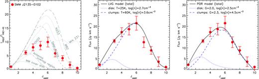
The integrated 12CO SLED for SMM J2135 showing that the SLED peaks around Jupper = 6 (similar to M 82, but with proportionally stronger 12CO(1–0)). The central panel shows the results of LVG modelling applied to the integrated SLED, which requires two temperature phases to yield an adequate fit. In this model, they have characteristic temperatures of Tkin = 25 and 60 K and densities of n = 102.7 and 103.6 cm−3, respectively (we associate these two phases with a cool, extended disc and hotter, more compact, clumps). The right-hand panel shows a similar comparison but now using a PDR model (Meijerink et al. 2007; see Section 3.2.1), which again requires a combination of both low- and high-density phases to adequately fit the integrated SLED.
3.1 Integrated properties
3.1.1 Gas mass and dust spectral energy distribution
We begin by estimating the total molecular gas mass of the galaxy from 12CO. Low-Jupper transitions of 12CO are commonly used to obtain estimates of the total gas mass of a galaxy using a conversion factor,  (K km s−1 pc2)−1, which converts the 12CO line luminosity to total gas mass, (where
  is defined to include the mass of helium, such that
  ; see Solomon & Vanden Bout 2005 for a review).
 K (TCMB = 2.73 K at z = 0), z = 2.3259, g1 = 3 (the degeneracy of level n = 1), Z∼ 2(Tk/T0) and [12CO/H2]∼ 10−4 for a solar metallicity environment (Bryant & Scoville 1996). For typical star-forming gas, Tk∼ 40–60 K, so to derive a minimum mass, we use Tk = 40 K. With
  K km s-1 pc2, this gives us a minimum gas mass of Mgas≳ 1 × 10¹⁰ M⊙ and a lower limit on α≳ 0.54.
We can then compare this to the dynamical mass adopting Mdyn = 5Rσ2/G (Solomon & Vanden Bout 2005). This assumes that the dynamics of the CO emission trace the virialized potential well of the system and that the CO is distributed in a sphere of constant density with r∼ 1 kpc (see Section 3.4 and Swinbank et al. 2010). Using the width of the 12CO(1–0) line, σ∼ 200 km s−1, we estimate a dynamical mass of Mdyn∼ 5.3 × 10¹⁰ M⊙. If this mass is dominated by gas, then the upper limit on α is  .
.
Using this dynamical mass and the minimum gas mass, we place a lower limit on the gas fraction of Mgas/Mdyn≳ 0.19. This ratio is similar to the ratio for typical starburst nuclei and the ratio of 30 per cent found in M 82 (Devereux et al. 1994). Compared to other high-redshift submillimetre galaxies (SMGs), using the 12CO(3–2) observations from Greve et al. (2005) and adopting α = 0.8 and R3,1 = 0.58 ± 0.05 from Ivison et al. (2010c), we find a median gas mass ratio of 50 per cent for luminous SMGs, whilst Tacconi et al. (2008) derived a gas mass fraction of 0.3 for more typical star-forming galaxies at similar redshifts. We stress, however, that compared to the gas mass of 6 × 10⁸ M⊙ within the central 1.2 kpc of M 82 (Young & Scoville 1984), our gas mass is nearly two orders of magnitude higher, underlining the more extreme conditions in the central regions of SMM J2135.
In order to provide a simple comparison with previous studies, we estimate the gas mass of SMM J2135 using a conversion factor of α∼ 0.8 which applies to the smoothly distributed, high-pressure, largely molecular ISM measured in local ULIRGs (Downes & Solomon 1998; Solomon & Vanden Bout 2005, although recent local studies on high-Jupper CO lines imply multiphase ISM in ULIRGs as opposed to smoothly distributed) and is also the canonical value used for high-redshift LIRGs and ULIRGs (Stark et al. 2008; Tacconi et al. 2008). This value of α is comfortably between the upper and lower limits calculated above. With this assumption, the 12CO(1–0) line luminosity yields a total gas mass of  (see also Swinbank et al. 2010).
Taking our estimate of the total gas mass and the expected size of ∼1 kpc for the system (Swinbank et al. 2010), we derive an average column density of ∼ 1024 cm−2, which is comparable to the molecular hydrogen density in Arp 220, averaged over a similar region (Gerin & Phillips 1998), but much higher than the density in typical starburst galaxies, such as M 82. However, this estimate gives an average over the system which we know to be structured and so indicates that the column density is very high in parts of this source. The associated extinction is expected to exceed AV∼ 103, suggesting significant absorption even in the far-IR and moreover that the emission from some of the more common species we see is optically thick. With this extinction, coupled with our high value for G0 (derived in Section 3.2.1), high-IR luminosity and potentially high cosmic-ray flux (see below), it is probable that momentum-driven outflows will result. These outflows could be either photon-driven (Thompson, Quataert & Murray 2005) or cosmic ray driven (Socrates, Davis & Ramirez-Ruiz 2008) and will impact both the dynamics of the gas in the system and the steady-state assumption in our PDR modelling (Section 3.2.1).
We can now compare the star formation efficiency (SFE) in SMM J2135 to that in the wider SMG and ULIRG populations. First we note that the far-IR luminosity of SMM J2135 is LFIR = (2.3 ± 0.1) × 1012 L⊙ (Ivison et al. 2010b), which indicates an SFR of ∼ 400 ± 20 M⊙ yr−1 (Kennicutt 1998) assuming a Salpeter IMF. We combine the SFR and gas mass to estimate the SFE following Greve et al. (2005),  resulting in SFE ∼ 165 ± 7 L⊙ M−1⊙. This is comfortably within the limit derived by Scoville (2004) of [
 ]max = 500 L⊙ M−1⊙, assuming Eddington-limited accretion of gas on to OB star clusters. 12CO(1–0) measurements in local ULIRGs derive an SFE of 180 ± 160 L⊙ M−1⊙, which is comparable to that in our source. The SFE of our source is also comparable to the median SFE of 210 ± 80 L⊙ M−1⊙ for the sample of luminous SMGs of Greve et al. (2005), after correcting the latter using R3,1 = 0.58 as appropriate for SMGs (Harris et al. 2010; Ivison et al. 2010c).
We begin modelling this system by noting that the 870-μm SMA observations and comparison to the LABOCA flux reveal four bright, compact clumps embedded in a much more extended system with the clumps emitting ∼80 per cent of the total luminosity, and the rest of the emission emerging from a more extended component (Swinbank et al. 2010). Motivated by this structure, we fit a two-component model to the dust spectral energy distribution (SED), fixing the characteristic temperature of the cool (presumably more extended) component at 30 K and allowing the size and the characteristic temperature of the clumps to vary. The best fit yields a characteristic size for the clumps of r∼ 200 pc at a temperature of Td,warm = 57 ± 3 K, while the extended component has a size of r∼ 1000 pc at Td,cool = 30 K. The dust mass of both the extended component and the clumps is then (1.5 ± 0.2) × 108 M⊙, which is similar to the mass determined for the cool dust component in Ivison et al. (2010b). The inferred clump size is somewhat larger than the size of the dust emission regions seen in the highest resolution 870-μm SMA maps, where the clumps appear to be 100–200 pc in diameter (Swinbank et al. 2010). However, we note that forcing the clump sizes down to that size requires an increase in the characteristic temperature up to ∼80 K, and to keep the emission consistent with the integrated SED, the clumps must then be optically thick at ∼ 200 μm in the rest-frame. Clearly this two-component model is not a unique description of the dust emission from SMM J2135, but it does suggest that the system could be modelled by a combination of warm, compact and cooler, more extended dust component.
3.1.2 12CO SLED
To investigate the excitation within the ISM, we next construct the 12CO SLED by calculating the 12CO flux of each transition over the velocity range defined by the composite spectrum; we show the resulting SLED in Fig. 2. In Table 4 (see later), we also give the velocity-averaged brightness temperature ratios between 12CO(Jupper) and 12CO(1–0), which we define as RJ,1=L′ (J+ 1 → J)/L′ (1 → 0) (Greve, Ivison & Papadopoulos 2003; Harris et al. 2010). The 12CO SLED shows a continuous rise out to Jupper = 6, followed by a sharp decline as far as Jupper = 10. The brightness ratios of all of the Jupper > 2 line luminosities compared to the 12CO(1–0) are <1, which interpreted in the framework of a single phase ISM would indicate that the gas is subthermalized (the thermalized prediction is ∼1; Devereux et al. 1994). Indeed the  line luminosity ratio for SMM J2135, 0.68 ± 0.03, is similar to that seen in local starburst galaxies, 0.64 ± 0.06 (Devereux et al. 1994). However, as Harris et al. (2010) discuss and as we show later in Section 3.2, these ratios are more likely to indicate a multiphase ISM as found in star-forming regions locally.
Line ratios.
| Component |  (109 M⊙) (109 M⊙) | R3,1a | R4,1 | R5,1 | R6,1 | R7,1 | R8,1 |  |  |
| Total | 40.0 ± 0.3 | 0.68 ± 0.03 | 0.50 ± 0.04 | 0.35 ± 0.02 | 0.28 ± 0.02 | 0.119 ± 0.008 | 0.064 ± 0.005 | 0.37 ± 0.02 | 0.41 ± 0.02 |
| Z | 10.1 ± 1.8 | 0.71 ± 0.19 | 0.42 ± 0.12 | 0.51 ± 0.11 | 0.41 ± 0.09 | 0.17 ± 0.04 | 0.09 ± 0.01 | 0.85 ± 0.21 | 0.32 ± 0.10 |
| Y | 23.1 ± 3.2 | 0.67 ± 0.14 | 0.49 ± 0.10 | 0.22 ± 0.05 | 0.19 ± 0.05 | 0.09 ± 0.02 | 0.04 ± 0.01 | 0.19 ± 0.05 | 0.43 ± 0.09 |
| X | 6.8 ± 3.2 | 0.70 ± 0.48 | 0.67 ± 0.42 | 0.48 ± 0.29 | 0.38 ± 0.23 | 0.06 ± 0.06 | 0.11 ± 0.06 | 0.43 ± 0.27 | 0.38 ± 0.28 |
| Component | (109 M⊙) | R3,1a | R4,1 | R5,1 | R6,1 | R7,1 | R8,1 | | |
| Total | 40.0 ± 0.3 | 0.68 ± 0.03 | 0.50 ± 0.04 | 0.35 ± 0.02 | 0.28 ± 0.02 | 0.119 ± 0.008 | 0.064 ± 0.005 | 0.37 ± 0.02 | 0.41 ± 0.02 |
| Z | 10.1 ± 1.8 | 0.71 ± 0.19 | 0.42 ± 0.12 | 0.51 ± 0.11 | 0.41 ± 0.09 | 0.17 ± 0.04 | 0.09 ± 0.01 | 0.85 ± 0.21 | 0.32 ± 0.10 |
| Y | 23.1 ± 3.2 | 0.67 ± 0.14 | 0.49 ± 0.10 | 0.22 ± 0.05 | 0.19 ± 0.05 | 0.09 ± 0.02 | 0.04 ± 0.01 | 0.19 ± 0.05 | 0.43 ± 0.09 |
| X | 6.8 ± 3.2 | 0.70 ± 0.48 | 0.67 ± 0.42 | 0.48 ± 0.29 | 0.38 ± 0.23 | 0.06 ± 0.06 | 0.11 ± 0.06 | 0.43 ± 0.27 | 0.38 ± 0.28 |
Masses and line luminosity ratios for individual kinematic components.
aRJ,1 represents L′CO(J+1−J)/L′CO(1−0).
Line ratios.
| Component | (109 M⊙) | R3,1a | R4,1 | R5,1 | R6,1 | R7,1 | R8,1 | | |
| Total | 40.0 ± 0.3 | 0.68 ± 0.03 | 0.50 ± 0.04 | 0.35 ± 0.02 | 0.28 ± 0.02 | 0.119 ± 0.008 | 0.064 ± 0.005 | 0.37 ± 0.02 | 0.41 ± 0.02 |
| Z | 10.1 ± 1.8 | 0.71 ± 0.19 | 0.42 ± 0.12 | 0.51 ± 0.11 | 0.41 ± 0.09 | 0.17 ± 0.04 | 0.09 ± 0.01 | 0.85 ± 0.21 | 0.32 ± 0.10 |
| Y | 23.1 ± 3.2 | 0.67 ± 0.14 | 0.49 ± 0.10 | 0.22 ± 0.05 | 0.19 ± 0.05 | 0.09 ± 0.02 | 0.04 ± 0.01 | 0.19 ± 0.05 | 0.43 ± 0.09 |
| X | 6.8 ± 3.2 | 0.70 ± 0.48 | 0.67 ± 0.42 | 0.48 ± 0.29 | 0.38 ± 0.23 | 0.06 ± 0.06 | 0.11 ± 0.06 | 0.43 ± 0.27 | 0.38 ± 0.28 |
Masses and line luminosity ratios for individual kinematic components.
aRJ,1 represents L′CO(J+1−J)/L′CO(1−0).
The peak of the SLED at Jupper = 6 is similar to that seen in nearby starburst galaxies, such as NGC 253 and M 82 (Bradford et al. 2003; Weiß, Walter & Scoville 2005c; Panuzzo et al. 2010), and active galactic nuclei (AGNs), such as Mrk 231 (Papadopoulos, Isaak & van der Werf 2007; van der Werf et al. 2010). However, the overall shape of the SLED suggests that SMM J2135 has proportionally stronger 12CO(1–0) emission (compared to the higher Jupper transitions) than any of these galaxies, indicating the presence of an additional low-excitation gas phase. Nevertheless, the bulk of the cooling, 60 per cent, arises through the 12CO Jupper = 5–7 line emission, with a further 20 per cent at 12CO Jupper≥ 8. van der Werf et al. (2010) have recently constrained the 12CO in Mrk 231 up to Jupper = 13 with Herschel, building upon the earlier study of Papadopoulos et al. (2007), and show that, unlike nearby starbursts (e.g. NGC 253 or M 82), the 12CO line luminosity is roughly flat across Jupper = 5–13. They calculate that only 4 per cent of the total 12CO line luminosity arises from the three lowest transitions, compared to ∼20 per cent in the three lowest transitions of our 12CO SLED (and 43 per cent in the Milky Way). The luminous high-Jupper emission they see is likely due to the presence of additional excitation phases in Mrk 231, either high-excitation PDRs or more likely an X-ray-dominated region (XDR) (Spaans & Meijerink 2008). As we see later, we also find evidence for at least two phases of material in SMM J2135.
In comparison to higher-redshift sources, we see that the 12CO SLED for SMM J2135 has a broadly similar shape to that seen in other high-redshift SMGs, for example, GN 20 (Carilli et al. 2010) or SMM J16359 (Weiß et al. 2005b). Indeed, recent progress with EVLA and GBT has started to provide 12CO(1–0) detections of SMGs to complement the earlier 12CO(3–2) studies from PdBI (e.g. Greve et al. 2005). Using these two transitions, we find that the R3,1 brightness temperature ratio we derive for SMM J2135 (Table 4) is comparable to typical SMGs: R3,1 = 0.55 ± 0.05 (Ivison et al. 2010c) and R3,1 = 0.68 ± 0.08 (Harris et al. 2010), suggesting that the CO SLED results we derive for SMM J2135 may be applicable to the wider SMG population.
To investigate the excitation of the gas reservoir within this galaxy in more detail we exploit the fact that the shape of the 12CO SLED can provide information on the underlying gas density and temperature distributions and use a spherical large velocity gradient model (LVG; Weiß et al. 2005b) to attempt to fit the observed SLED. LVG techniques are the most widely used radiative transfer model which can account for photon transport when spectral lines are optically thick, and can be used for efficiently solving the radiative transfer equation when the molecule level populations are not thermalized (Bayet et al. 2006).
Thus we next use the LVG code to model the 12CO SLED. The model assumes spherical symmetry and uniform kinetic temperature and density, a cosmic microwave background temperature of TCMB = 2.73 K (1 +z), which at z = 2.3 is ∼9 K, the collision rates from Flower (2001) with an ortho/para H2 ratio of 3 and a ratio of the CO abundance to the velocity gradient of CO/dv/dr = 10−5 pc (km s−1)−1. To fit absolute line intensities, the model further uses the source solid angle size, ΩS, which can be expressed in terms of the equivalent radius of a face-on disc,  . The model returns the temperature, density and size of the emission region.
Modelling the 12CO SLED in this way, we find that a single temperature and density phase is unable to fit the SLED, and that two or more phases are required. This is consistent with the implication of the model of the dust SED and the submillimetre morphology: we need at least two temperature phases to adequately describe this system. This need for multiple phases to fit the ISM in a high-redshift galaxy is unusual (cf. Carilli et al. 2010), although it is not unexpected given that such multiphase ISMs are commonly required in local galaxies (e.g. Wild et al. 1992; Guesten et al. 1993; Aalto et al. 1995; Mao et al. 2000; Ward et al. 2003). Thus, motivated by the fit to the dust SED we identify a two-phase fit to the SLED comprising four clumps and an extended phase, which provides an adequate fit (Fig. 2). In this model, the low-excitation phase peaks at Jupper∼ 3 and is diffuse, with n∼ 102.7 cm−3 and Tkin∼ 25 K. The denser, mildly excited phase peaks around Jupper = 5–6, has Tkin∼ 60 K and n∼ 103.6 cm−3 and contributes ∼60 per cent of the total luminosity over all the 12CO lines (Fig. 2). The low-excitation phase has a 12CO SLED which is very similar to the inner disc of the Milky Way, while the warmer phase is well matched to the inner few hundred parsecs of the starburst region in NGC 253. Within this two-phase model, the total gas mass is Mgas∼ (4.0 ± 0.1) × 1010 M⊙, a factor of ∼3 times the mass we determine from 12CO(1–0), assuming α = 0.8, corresponding to an effective α = 2.0 (simlar to that derived for the nucleus of Arp 220; Scoville, Yun & Bryant 1997). From here on, we adopt this value as the gas mass of our system, but note some of the differences if we had used the 12CO line luminosity and α = 0.8, as is commonly assumed in the analysis of high-redshift galaxies. The combination of this higher value for α and our estimate of R3,1 would increase the gas mass by a factor of ∼4 times over that estimated by assuming α = 0.8 and R3,1 = 1 as usually assumed at high redshift (see also Ivison et al. 2010a; Harris et al. 2010). Adopting α∼ 2 results in a gas mass fraction in the central 1-kpc radius region of SMM J2135 of 75 per cent (and closer to the 100 per cent for typical SMGs, Greve et al. 2005), subject to uncertainties on the dynamical mass due to the unknown configuration of the gas within the system.
3.1.3 Atomic carbon
We have also obtained strong detections of the [C i](3P1→3P0) and [C i](3P2→3P1) emission lines, and from these we can begin to investigate the properties of the ISM. We start by noting the similar detailed morphologies of the [C i](3P1→3P0) and the 12CO(3–2) and 12CO(1–0) lines in Fig. 1, which suggests that the emission is arising from the same mix of phases with characteristic temperatures of T≲ 40 K. Indeed observations of neutral carbon transitions have shown that the ratio of  provides a sensitive probe of the temperature of the ISM at moderate densities. Both lines have modest critical densities [ncrit∼ (0.3–1.1) × 103 cm−3] and are therefore often thermalized in molecular clouds with n≳ 103 cm−3. The lines arise from states with energy levels T1 = 23.6 K and T2 = 62.5 K above the ground state, and thus their ratio is sensitive to the gas temperature if Tgas≲ 100 K. We derive
  , which is similar to that measured in nearby starbursts and galactic nuclei, such as M 82 and NGC 253, where
 (Bennett et al. 1994; White et al. 1994; Israel, White & Baas 1995; Bayet et al. 2004), but larger than typically found in the cooler, dense cores of giant molecular clouds (GMC; e.g. Zmuidzinas et al. 1988). To be compatible with previous studies, we define
  as the ratio of the [C i](3P2→3P1) to [C i](3P1→3P0) temperature integrated line intensities in K km s−1. In SMM J2135, we derive an integrated line ratio of
  . We can use this ratio to estimate the excitation temperature Tex following Stutzki et al. (1997), Tex = 38.8 K/
 , and derive Tex = 44.3 ± 1.0 K for SMM J2135.
 is the [C i] partition function and Tex is defined above. Using Tex = 44.3 ± 1.0 K and our measured luminosity of the upper fine structure line, [C i](3P1→3P0), we estimate a carbon mass of M[C I] = (9.1 ± 0.2) × 106 M⊙. Combining this with our gas mass estimated from the LVG analysis, we derive a [C i] abundance of M([C i])/6M(H2) = (3.8 ± 0.1) × 10−5, which is higher than the Galactic value of 2.2 × 10⁻⁵ from Frerking et al. (1989). Similarly, the ratio of the [C i] and 12CO brightness temperatures,
 , falls towards the upper end of the range 0.2 ± 0.2 observed in local galaxies (Gerin & Phillips 2000; Bayet et al. 2006). A higher abundance of [C i] relative to 12CO is expected in regions with lower metallicity (Stark et al. 1997), where 12CO is photodissociated, in regions with a high ionization fraction, which may drive the chemistry to equilibrium at a high [C i]/12CO ratio, and in starburst systems with a high cosmic-ray flux (Flower et al. 1994; Papadopoulos, Thi & Viti 2004).
We can also attempt to model the [C i] emission within the framework of our two-phase LVG model. We find that we are only able to simultaneously fit the [C i] luminosities and ratios, if the carbon abundance is allowed to vary between the two phases. To fit the observed R ratio and the [C i] to 12CO brightness temperatures the LVG model suggests [C i/12CO] ∼ 0.2 for the warm, dense phase, which is close to the Galactic value, [C i]/12CO ∼ 0.13 (Frerking et al. 1989), while for the extended, low-density phase, we require an abundance of [C i]/12CO ∼ 3.0, which suggests a deficit of oxygen, and hence possibly a very low metallicity. Using the correlation between [C i]/12CO and metallicity (12 + log[O/H]) in Bolatto et al. (2000), for the cool component, we derive 12+log(O/H) = 7.5 and hence a metallicity of ∼Z/Z⊙ = 1/25. This is similar to that of the Sextans dwarf galaxy, to the lowest metallicity, young starbursts seen locally (Brown, Kewley & Geller 2008) and to the lowest metallicity galaxies found at high redshift (Yuan & Kewley 2009). However, the high [C i]/12CO ratio could also be due to a high cosmic-ray flux in the galaxy (Papadopoulos et al. 2004; Israel & Baas 2002). Indeed a factor of ∼10 times enhancement of cosmic-ray flux will yield the high [C i/12CO] ratio we observe and this may not be unlikely, given the high SFR density of the star-forming regions (Swinbank et al. 2010). Moreover, an enhanced [C i/12CO] ratio has also been observed in the starburst galaxy NGC 253 (Harrison et al. 1995; Bradford et al. 2003) attributed to a high cosmic-ray flux.
Finally, the [C i] detections can be combined with the observations of [C ii]157.7 from Ivison et al. (2010b) to investigate the ISM cooling. We can compare the cooling in each of our lines relative to the bolometric (8–1000 μm) luminosity, to assess their importance. The fraction of the bolometric luminosity in the [C ii] line is 0.24 per cent, the rotational 12CO lines [12CO(1–0) to 12CO(10–9)] contribute 0.09 per cent and the [C i] lines result in just 0.03 per cent. Therefore, [C ii] dominates the cooling with the total cooling due to 12CO and [C i] representing ∼50 per cent of the cooling due to [C ii]. [C ii] is one of the brightest emission lines in galaxies and can account for 0.1–1 per cent of the far-IR luminosity of the nuclear regions of galaxies (Stacey et al. 1991); our source lies well within that range. This situation is in contrast to comparably luminous systems in the local Universe, e.g. Arp 220, where the [C ii] emission is just 1.3 × 10⁻⁴ of LFIR (Gerin & Phillips 1998). This most likely results from saturation of [C ii] in very high-density star-forming regions (Luhman et al. 1998). The proportionally stronger [C ii] emission that we see in SMM J2135 may then indicate slightly lower densities in the system and more extended star formation (Ivison et al. 2010c), or it may be due to the lower metallicity of the gas compared to local ULIRGs (Israel et al. 1996; Maiolino et al. 2009).
Overall, our observations of atomic carbon suggest that it arises from a cool phase within the galaxy and that integrated over the whole galaxy the [C i]/12CO ratio is higher than the Galactic value. However, we also find evidence for variation in the ratio within the system, with the cool, low-density phase having significantly enhanced [C i], compared to 12CO, suggesting lower metallicity in this phase or a higher cosmic-ray flux in the overall system.
3.1.4 HCN(3–2)
Our spectra also cover emission lines from a number of species other than 12CO; notably, we detect HCN(3–2) emission (Table 2). HCN is an effective tracer of dense gas due to its high dipole moment, requiring ∼100 times higher densities for collisional excitation than 12CO(1–0). Indeed, HCN is one of the most abundant molecules at densities n≳ 3 × 104 cm−3 (compared to critical densities of ≳500 cm−3 for low-Jupper levels of 12CO). We note that the velocity centroid of the HCN emission is redshifted by approximately +230 ± 100 km s−1, relative to the nominal systemic redshift of the system derived from 12CO. As we discuss below, this hints that the HCN emission may arise predominantly from only one of the kinematic components within the galaxy.
It has been shown that the HCN line luminosity is tightly correlated with far-IR luminosity in local spirals and ULIRGs, with a linear relation holding over at least three decades in luminosity, and a similar relation may hold at high redshift (Fig. 3; Gao & Solomon 2004; Gao et al. 2007). This suggests that HCN is a good tracer of the dense gas which fuels the massive star formation, which in turn is responsible for the far-IR emission. In Fig. 3, we show the relation between far-IR luminosity and HCN(3–2) line luminosity for local spirals, LIRGs and ULIRGs (Gao & Solomon 2004; Juneau et al. 2009). SMM J2135 lies at the high-luminosity end of this correlation, corresponding to the highest-luminosity local ULIRGs, and is consistent with the relation. In the inset panel on Fig. 3, we also compare our source to local LIRGs and ULIRGs in Gao & Solomon (2004). We show the upper limit on  using our 3σ upper limit for HCN(1–0) flux, demonstrating that this is also consistent with the increasing
  ratio seen with increasing LFIR at low redshift.
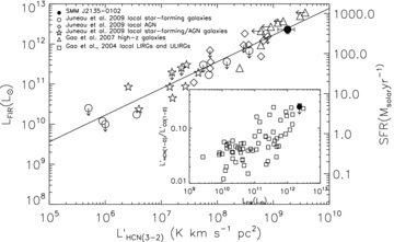
The relation between far-IR luminosity and HCN luminosity for galaxies. We compare our observations of SMM J2135 with the correlation seen locally and find that this high-redshift galaxy follows the tight correlation seen in local galaxies (Juneau et al. 2009). In the main panel, we plot observations from a sample of 34 local galaxies (star-forming galaxies, star-forming galaxies with AGNs and strong AGNs) taken from Juneau et al. (2009). In the inset panel, we compare our upper limit on the ratio of  to the ratio in local LIRGs and ULIRGs from Gao & Solomon (2004) showing that this upper limit is consistent with the Gao & Solomon (2004) relation. Again we see that the properties of the dense gas and far-IR emission in this galaxy are similar to those seen locally.
It is also possible to estimate a total gas mass from the HCN luminosity (Gao, Springel & White 2005). Using our 3σ upper limit on the HCN(1–0) luminosity, we derive a limit on the dense gas mass of Mdense(H2) =αHCN(1-0)L′HCN≪ 4.5 × 10¹⁰ M⊙ with αHCN≪ 10 (Gao & Solomon 2004). We caution that there is at least a factor of 3 times uncertainty arising from the uncertainty in αHCN. The value of αHCN we adopt is appropriate for a virialized cloud core; however, ULIRGs and LIRGs usually have a much higher HCN brightness temperature, resulting in their αHCN being much lower (Gao & Solomon 2004), and hence this is reported as an upper limit on the gas mass. Since this gas mass is consistent with the mass derived from our LVG analysis of 12CO, this suggests that with better estimates of αHCN, HCN may be a promising route to constraining the dense gas masses of high-redshift galaxies in the future. However, we note that the consistency of 12CO-based and HCN-based gas mass estimates may be coincidental if these lines trace different phases. We further caution that at least two HCN lines may be required to derive the correct value of αHCN due to the strong variations in HCN(4–3)/HCN(1–0) and HCN(3–2)/HCN(1–0) luminosity ratios locally (Papadopoulos 2007).
As with [C i], we also attempted to use our two-phase LVG model from the 12CO SLED to model the HCN(3–2) and HCN(1–0) emission from this system. However, we find that any models, which fit the HCN SLED, in particular the bright HCN(3–2) emission, overpredict the luminosities of the 12CO SLED and result in gas masses, which are greater than the dynamical mass. A similar problem has been identified in local ULIRGs which exhibit enhanced HCN line emission and high ratios of L′HCN / due to a higher proportion of dense gas in these strong starburst systems (Solomon & Vanden Bout 2005; Gao et al. 2007).
3.1.5 H2O
Finally, we comment on the limits obtained for H2O. H2O emission arises from the warm, dense gas in the densest regions of a starburst or around an AGN. The strength of the emission is thus a probe of the radiation density and so reflects the compactness of the far-IR source. The H2O (21,1–20,2) (731.681 GHz) emission line has recently been detected in the local ULIRGs, Mrk 231 and Arp 220 (e.g. González-Alfonso et al. 2010), revealing warm, dense material, possibly arising from an XDR associated with AGN activity (see also Spaans & Meijerink 2008 and van der Werf et al. 2010). We compare our limits on the H2O line luminosities (as a fraction of the bolometric luminosity) with Mrk 231 and Arp 220, where the luminosity ratios are  . We derive limits on the line luminosity ratio of
  from the H2O (51,5–42,2) and H2O (21,1–20,2) transitions. These suggest that if an XDR exists within SMM J2135 it is unlikely to be more luminous than those seen in these local AGN-dominated ULIRGs. This conclusion is reinforced by the relatively low luminosity of the high-Jupper12CO lines in SMM J2135 compared to the substantially brighter high-J lines in Arp 220 and Mrk 231 which again require an XDR to fit their 12CO SLEDs (Spaans & Meijerink 2008; van der Werf et al. 2010).
3.2 Integrated properties: physical properties of the ISM
When massive stars are formed around a molecular cloud, their UV radiation changes the chemical properties of the cloud's surface layers; the far-UV flux photodissociates the outer layer and ionizes the material (such as carbon). This layer then cools primarily via atomic fine structure lines of [O i], [C ii], [C i] and the rotational 12CO lines. Emission from these different coolants arises from different depths within the PDR (Kramer et al. 2004), such that the surface layers are dominated by emission from hydrogen, [C ii] and oxygen, although further into the star-forming clouds (as the extinction, AV, increases), hydrogen becomes molecular, whilst the ionization of carbon declines, with [C ii] becoming [C i] and then combining into CO. Moreover, with increasing density, the higher-Jupper12CO emission becomes stronger, as do other molecular gas tracers, such as HCN, CS and CN (Kaufman et al. 1999). Deeper into the cloud, the gas is molecular, but still has a higher temperature than in the far-UV shielded core. Significant effort has been devoted to modelling (and predicting) the fine structure and molecular emission-line ratios associated with these star-forming regions using PDR models. These account for variations in density, temperature, clumpiness and time-dependent chemistry (e.g. Kaufman et al. 1999; Meijerink, Spaans & Israel 2007) and using their predictions of the ratios of [C ii], [C i] and 12CO, we can investigate the typical far-UV intensity and ISM density within the star-forming regions in SMM J2135.
3.2.1 PDR models
To model the full-range of observed line ratios from SMM J2135, we use the PDR models of Kaufman et al. (1999) and Meijerink et al. (2007) in which the emission is determined by the atomic gas density (n; the density of H nuclei) and the incident far-UV radiation field from massive stars (hν = 6–13.6 eV) which is expressed in terms of G0 (where G0 is the average far-UV radiation field in the Milky Way and is expressed in Habing units: 1.6 × 10⁻³ erg s−1 cm−2). Simple PDR models (including one of the two models we compare to; Kaufman et al. 1999) calculate the line emission generated by a cloud illuminated only on one side. However, for observations of external galaxies it is not clear that such a ‘single cloud’ model will adequately describe the observed molecular lines. For clouds illuminated on all sides, we note that an observer will detect optically thin radiation emitted from both the near and far sides of the cloud, but only see optically thick emission from the near side. Generally, low-Jupper12CO transitions are assumed to be optically thick for the nominal AV = 10 cloud depths in the PDR models (Hailey-Dunsheath et al. 2010b), whilst [C ii], [C i], 13CO and LFIR are assumed to be optically thin (although note our earlier estimates of the high column densities and extinction in this system). We have not applied any corrections to the emission lines to account for these differences between optically thick and optically thin emission. Instead, we also compare to more complicated models involving two or more clouds, with differing densities and incident radiation fields which have been constructed by Meijerink et al. (2007). The implementation of these models assumes that all emission lines are coming from the same gas in the same region, which we know to be a vast oversimplification; however, these solutions do provide us with order of magnitude estimates of the characteristic conditions in the system.
In Fig. 4, we show the model grid of n and G0 values for various emission-line ratios for SMM J2135. The 12CO J/(J− 1) and [C i]/12CO line luminosity ratios vary over six orders of magnitude in G0; however, the [C ii]/FIR and [C ii]/12CO ratios appear to break this degeneracy. Indeed, in the n∼ 103–105 cm−3 regime, these provide a strong constraint on G0. Using the two different PDR models we convert the allowed parameter space for each line ratio to derive the peak likelihood solution, which is shown in Fig. 4 for both models. We find that the solutions cluster around moderate densities (n∼ 104 cm−2), similar to those claimed for local ULIRGs from PDR modelling of H2 emission (Davies et al. 2003). The peak likelihood solutions use all the line ratios available aside from the  ratio. This line's track deviates strongly from the preferred solution from the other lines. We expect this reflects the sensitivity of this line ratio to details of the PDR, such as geometry, and we discuss specific problems with the PDR model treatment of [C i] below.
![Left-hand panel: luminosity line ratios (in units of L⊙) from 12CO, [C i] and [C ii] as a function of density and far-UV flux (G0 in units of Habing field), from the PDR models of Kaufman et al. (1999). Tracks are drawn for the measured ratios in solid lines with the 1σ errors as dotted lines. The line ratios within SMM J2135 intercept at n∼ 104.1 cm−3 and G0∼ 103.6 Habing fields and n∼ 104.3 cm−3 and G0∼ 103.3 Habing fields for the Kaufman et al. (1999) and Meijerink et al. (2007) models, respectively. To better display the preferred regions of parameter space we combine the probability distributions from all of these lines [excluding L[C I](2-1)/L[C I](1-0) for reasons explained in Section 3.2] to derive a peak likelihood solution for each model. Right-hand panel: the same parameter space for the models, now comparing the peak likelihood solutions from the model grids to the derived values of G0 and density (n) for various low- and high-redshift galaxies and molecular clouds. We also indicate the regions of parameter space which are typically encompassed by Galactic OB star formation regions, starburst galaxies and non-starburst and Galactic molecular clouds from Stacey et al. (1991). This shows that the line ratios for SMM J2135 are consistent with those typically found in local starbursts or ULIRGs. The local galaxy that lies within the contours of the peak likelihood for the Kaufman models is NGC 253, a spiral starburst galaxy (Negishi et al. 2001). We also show the peak likelihood solution derived from the PDR models of Meijerink et al. (2007), which provide a concomitant solution. The contours represent the 1σ and 2σ limits compared to the best-fitting solution. The peak likelihood solutions are derived without including the L[C I](2-1)/L[C I](1-0) track, which we plot on both panels to show its discrepancy from the general solution from the other lines (see Section 3.2).](https://oup.silverchair-cdn.com/oup/backfile/Content_public/Journal/mnras/410/3/10.1111/j.1365-2966.2010.17549.x/2/m_mnras0410-1687-f4.jpeg?Expires=1750252867&Signature=g8dz5ItdvTeGLFl3ZgA46u3YFzEkYLVnL3sEkg6bF~DZ750AAC2AflgbFSajyonL3rTf-mH4Uis1TjSNbc1kOAm6Q~XrNm3X0bndLasPzaZ5TZqyX8tu9ccUXkTf-xurqFvywTU8vTrkISN~WBpCP2m3VVHhKio45JXHJ6LRNVtXEm0T7PhVQ2JXRGxVnrYQPZroDGJti4lq-UHaWDKWAsFXQOEwX0ibNnFC9bWGQglAk8VaaVAD6ubPIx0xIxPU-VouSp0JCEBaXVMA921Ysgf3YVXpAv9z1gjwZrD6A~60dYTnBd24QDy-Uknv1wDnotxAc4fnLWCYlE1dPJDcWA__&Key-Pair-Id=APKAIE5G5CRDK6RD3PGA)
Left-hand panel: luminosity line ratios (in units of L⊙) from 12CO, [C i] and [C ii] as a function of density and far-UV flux (G0 in units of Habing field), from the PDR models of Kaufman et al. (1999). Tracks are drawn for the measured ratios in solid lines with the 1σ errors as dotted lines. The line ratios within SMM J2135 intercept at n∼ 104.1 cm−3 and G0∼ 103.6 Habing fields and n∼ 104.3 cm−3 and G0∼ 103.3 Habing fields for the Kaufman et al. (1999) and Meijerink et al. (2007) models, respectively. To better display the preferred regions of parameter space we combine the probability distributions from all of these lines [excluding L[C I](2-1)/L[C I](1-0) for reasons explained in Section 3.2] to derive a peak likelihood solution for each model. Right-hand panel: the same parameter space for the models, now comparing the peak likelihood solutions from the model grids to the derived values of G0 and density (n) for various low- and high-redshift galaxies and molecular clouds. We also indicate the regions of parameter space which are typically encompassed by Galactic OB star formation regions, starburst galaxies and non-starburst and Galactic molecular clouds from Stacey et al. (1991). This shows that the line ratios for SMM J2135 are consistent with those typically found in local starbursts or ULIRGs. The local galaxy that lies within the contours of the peak likelihood for the Kaufman models is NGC 253, a spiral starburst galaxy (Negishi et al. 2001). We also show the peak likelihood solution derived from the PDR models of Meijerink et al. (2007), which provide a concomitant solution. The contours represent the 1σ and 2σ limits compared to the best-fitting solution. The peak likelihood solutions are derived without including the L[C I](2-1)/L[C I](1-0) track, which we plot on both panels to show its discrepancy from the general solution from the other lines (see Section 3.2).
The best-fitting solution to our suite of line ratios is n = 104.1±0.3 cm−3 and G0 = 103.6±0.7 Habing fields for the PDR models from Kaufman et al. (1999) and n∼ 104.3±0.2 cm−3 and G0∼ 103.3±0.2 Habing fields from Meijerink et al. (2007). The best-fitting solutions are within 1σ and are in agreement with earlier estimates based on just 12CO(1–0), [C ii] and LFIR in Ivison et al. (2010b). As we see from Fig. 4, these physical conditions are similar to local starburst galaxies and ULIRGs (Stacey et al. 1991; Davies et al. 2003) and at the upper end of both density and G0 for normal star-forming galaxies (Malhotra et al. 2001), for example, the radiation field is ∼1000 times more intense than in the disc of the Milky Way. The characteristic density compares well to the dense star-forming cores of Galactic molecular clouds, or to the central compact nuclear gas discs of local ULIRGs, such as Arp 220 (Downes & Solomon 1998; Sakamoto et al. 1999), and is also consistent with the integrated 12CO SLED (see Section 3.1.2). This characteristic density we derive is greater than the critical density for [C ii], [C i] and CO(1–0), above which the intensity of the lines saturates. Similarly, the G0 value we derive suggests the conditions in the PDRs are at the limit of the steady state solution (Kaufman et al. 1999); with radiation pressure on grains comparable to turbulence, suggesting that the PDRs may be ionizing material.
Our results imply that the underlying physics of the star formation occurring in the system is similar to the dense star-forming cores of Galactic molecular clouds (characteristic of massive OB star-forming regions), even though the total energetics of the system is far more extreme than in the disc of our galaxy. Interestingly, Teyssier, Chapon & Bournaud (2010) have recently used hydrodynamic simulations of major mergers of disc galaxies to show that the density of gas at which a majority of the star formation in these systems occurs is n∼ 104 cm−3, as we find here.
Of all the line ratios we analyse, the most obvious outlier in the PDR modelling is the [C i](3P2→3P1)/[C i](3P1→3P0) emission-line ratio (Fig. 4). However, we note that this line ratio is one of the most sensitive to G0 and n and it would only require a modest increase in the predicted [C i](3P1→3P0) flux in the models, ∼3 times stronger, to shift this track into agreement with the solution based on the bulk of the other ratios at n∼ 104 cm−3 and G0∼ 103.5. This problem may arise because the PDR models assume a particular geometry, which determines the ratio of diffuse to dense gas, and assume a homogeneous medium (an unrealistic assumption for our source). The resulting luminosity ratios based on 12CO/[C i] and [C i] are sensitive to this geometry and the [C i](3P2→3P1)/[C i](3P1→3P0) ratio is particularly sensitive to the homogeneity of the medium (Spaans 1996), as demonstrated by the difficulty the models have in reproducing the [C i](3P1→3P0) or [C i](3P2→3P1) emission lines even in tranquil environments (e.g. Pineda & Bensch 2007; Papadopoulos & Greve 2004). Indeed, Papadopoulos & Greve (2004) argue that [C i] is distributed relatively ubiquitously in molecular clouds (the critical density for excitation of both [C i](3P1→3P0) and [C i](3P2→3P1) is roughly that of 12CO(1–0); Solomon & Vanden Bout 2005). This is contrary to PDR theory, which places [C i] in a narrow [C ii]/[C i]/12CO transition zone on the surface of far-UV illuminated molecular clouds, and potentially makes [C i] a very effective tracer of H2 mass. Therefore our low ratio may be arising from geometrical optical depth effects in which the [C i] effectively follows the volume (rather than the PDR surface), which would naturally lower the [C i](3P2→3P1) /[C i](3P1→3P0) ratio (e.g. see Kramer et al. 2008) as would happen from any process, which enhances [C i] emission through the cloud's volume (e.g. cosmic rays). We also caution that the [C i](3P2→3P1) /[C i](3P1→3P0) ratio has been measured in only a few local galaxies (e.g. Bayet et al. 2006) and so the fine structure excitation of neutral carbon has yet to be fully characterised and calibrated locally.
3.2.2 Limits on 13CO, CN, HNC and HCO+
Our observations have also simultaneously covered a number of dense gas tracers and from these we can place limits on the line luminosities of 13CO, CN, HNC and HCO+. We can then ask if these limits are consistent with our preferred characteristic density and UV radiation field from the PDR model.
First we consider the limits on the 13CO. The 13C nuclei are synthesised by CNO processing of 12C nuclei from earlier stellar generations (12C is produced from He burning on rapid time-scales in massive stars). Since 13C is produced more slowly in intermediate mass stars during the red giant phase (at ∼1 Gyr), the 12C/13C ratio has been proposed as a diagnostic of the nucleosynthesis history in galaxies. A high ratio would then be seen at high redshift as the young starbursts will have had insufficient time to form secondary nuclei of 13CO. In the Milky Way and nearby star-forming galaxies, the 12CO/13CO line luminosity ratio ( ) is ∼5–10. However, local ULIRGs have shown a deficiency of 13CO (possibly due to gas inflow; Rupke, Veilleux & Baker 2008), which raises the 12CO/13CO line ratio to ∼30 (Greve et al. 2009). Indeed, recently, Henkel et al. (2010) showed that the 12CO/13CO luminosity line ratio in the Cloverleaf quasar (z = 2.6) is
  , suggestive of a deficiency of 13CO. Within SMM J2135, we estimate limits on the ratio of >5.8 and >6.5 for the Jupper = 1 and 3 transitions, respectively. These limits are consistent with the Milky Way, but more sensitive observations are required to place firm conclusions as to whether a deficiency exists similar to that observed in other local ULIRGs and high-redshift galaxies.
We can compare these limits to the predictions from the PDR models of Meijerink et al. (2007). The model predictions are  /
/ and 2.08 for the Jupper = 1 and 3 transitions, respectively, indicating lower 13CO abundance in SMM J2135 than the model predicts. This may arise due to a number of effects. It is known that the line luminosity ratios of giant molecular clouds are lower than galaxy-integrated properties due to the lower opacity of 13CO compared to 12CO in the intercloud medium. Since we are measuring galaxy integrated properties, this would naturally lower the ratio.
Clearly it would be useful to obtain a more sensitive observation of the 13CO to determine the extent of this discrepancy with PDRs.
Finally, we note that the line luminosity ratio of the dense gas tracers of CS(2–1)/12CO(1–0) < 0.13 is lower than that predicted from the PDR model (0.43). In contrast, the HNC(3–2)/12CO(1–0) < 1.3 and HCO+(3–2)/12CO(1–0) < 1.2 are consistent with those predicted by the PDR models (1.3 and 0.15, respectively). A more detailed test of the model prediction for these dense gas tracers will again require more sensitive observations.
3.3 Kinematically resolved properties: decomposed 12CO SLED
With the high S/N of our observations of 12CO and [C i] in Fig. 1, it is obvious that the spectra show significant kinematic structure and that more intriguingly this structure appears to vary between the different transitions and species. We therefore attempt to fit a model to the 12CO spectra and extract 12CO SLEDs for each kinematic component, in order to search for excitation structure within the system.
To construct a kinematic model for the 12CO emission, we fit the composite spectrum (Fig. 1) with a series of increasingly complex models. We find that a double Gaussian profile fit provides a ∼14σ improvement over a single Gaussian profile, with a triple profile giving a further ∼6σ improvement over the double Gaussian profile. Although this model reasonably describes the line profile of the system, P. Cox et al. (in preparation) use the velocity structure from high-resolution interferometry with PdBI up to Jupper = 7 to derive a map of the dynamics of SMM J2135 on ∼100-pc scales. The system can be described by two interacting discs: the lower-redshift of these displays a double-horned profile (termed Z1 and Z2), with a second, Y, at higher velocity which appears to connect to a further structure, X, extending to much higher velocity. Based on this interpretation we construct a model which comprises three components: two single Gaussians representing X and Y and a double-Gaussian for Z (constrained to have equal line widths and intensities for the two components). We fit this model to the composite spectrum, allowing the intensity, width and velocity of each component to vary and show the resulting best fit to the average line profile in Fig. 1 and report its parameters in Table 3. This fit has a χ2 of ∼20 for seven degrees of freedom and provides an adequate description of the composite line profile.
Model kinematic parameters.
| Component | v (km s−1) | σ (km s−1) |
| Z2 | −167 ± 9 | 75 ± 8 |
| Z1 | 28 ± 9 | 75 ± 8 |
| Y | 165 ± 13 | 157 ± 17 |
| X | 396 ± 9 | 76 ± 9 |
| Component | v (km s−1) | σ (km s−1) |
| Z2 | −167 ± 9 | 75 ± 8 |
| Z1 | 28 ± 9 | 75 ± 8 |
| Y | 165 ± 13 | 157 ± 17 |
| X | 396 ± 9 | 76 ± 9 |
Notes: Velocities and linewidths of the three kinematic components seen in the CO and [C i] spectra. The velocities are given with respect to a heliocentric redshift of z = 2.325 91.
Using the best-fitting model parameters from the composite 12CO spectrum, we apply the fit to each 12CO spectrum in turn, in order to extract the SLEDs for the three components in the model. Beginning with the average model parameters, we perturb the best fit randomly by up to ±20 km s−1 and fit this new realization to each of the 12CO spectra in turn, allowing only the relative intensities of the components to vary. We then sum the χ2 for the fit to each line for each model and determine the parameters for which the total χ2 is a minimum. We show the best-fitting model's line profile on each line in Fig. 1 and report their parameters in Table 3. To calculate errors, we allow the best-fitting parameters of the kinematic model to randomly vary (by their 1σ uncertainties) and run 105 Monte Carlo simulations, determining the 1σ variance in the range of fluxes from those models where the total χ2 of the model fit is within Δχ2 = 21 of the best fit (since we have seven emission lines and fit with three free parameters to each line). The errors on the parameters for the model fit to the average (velocity and dispersion in Table 3) are calculated using the standard deviation of the parameters for all models for which the total χ2 of the model fit is within Δχ2 = 21 of the best fit; these are quoted in Table 3.
The 12CO SLEDs for the three individual components are shown in Fig. 5. We derive the gas masses for each component using the 12CO(1–0) emission line and assuming our effective conversion factor α = 2.0 and list these in Table 4. The most highly excited components are X and Z, peaking at Jupper∼ 6 and containing ∼15 and ∼25 per cent of total gas mass, respectively (Table 4). Component Y, which we associate with the core of the second interacting system, is somewhat less excited, peaking at Jupper∼ 4, and contains most of the gas in the system (∼60 per cent of the total gas mass and a majority of the cold gas).
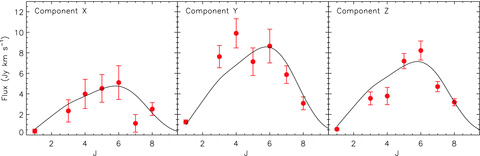
The 12CO SLEDs for the three kinematic components seen within the 12CO spectra (from the left-hand to right-hand side for the components at X, Y and Z at ∼−180, 0 and +200 km s−1, respectively). We overplot on each of these a scaled version of the best-fitting LVG model from the combined SLED. This shows that two components, X and Z, also peak at around Jupper∼ 6, while component Y appears to peak slightly lower, Jupper∼ 4, suggesting that there may also be temperature differences between the kinematic sub-components within the galaxy. Interestingly, component Y also appears to contain the bulk of the cold gas as traced by 12CO(1–0) compared to either X or Z.
For each of the SLEDs, we perform further LVG modelling as applied to the combined spectrum. However, within the errors, we cannot measure any temperature difference between the three components although there is a hint that Y is cooler than X or Z. However, while the [C i](3P2→3P1) and [C i](3P1→3P0) lines have lower S/N than the 12CO lines, we can also decompose them using the same method. Table 4 shows the ratio of  for the different components, with Z having the largest ratio and Y having the smallest. The corresponding excitation temperatures are Tex > 100, Tex = 24.7 ± 0.5 and Tex = 52.5 ± 6.3 K for Z, Y and X, respectively (where the temperature calculated for the Z component may be discrepant and likely caused by a problem with the model fit to the line; see Fig. 1). This supports the suggestion from the 12CO SLED that both X and Z are hotter than the more massive Y.
3.4 Physical interpretation
Swinbank et al. (2010) show that the rest-frame ∼250-μm emission from SMM J2135 is concentrated in four bright, star-forming regions each of which has a radius of ∼100 pc spread across a more diffuse structure with a total extent of 2 kpc in projection. Following this we fitted the integrated dust SED of the source (see Section 3.1.1) assuming that ∼20 per cent of the 870-μm flux is coming from a relatively cool (Td∼ 30 K) extended dust component with a predicted radius of ∼1 kpc and ∼80 per cent emerges from the four ∼100-pc radius, hotter (Td∼ 60 K) and optically thick, clumps. Our modelling of both the 12CO SLED and the kinematically decomposed [C i] line ratios supports the presence of two phases in the ISM within this galaxy with a cool, 15–25 K, phase and a hotter, 45–60 K, phase (although it is likely that these actually represent a continuum of properties). We also find an enhancement in the [C i]/12CO ratio (likely due to low metallicity and/or higher cosmic-ray flux) which is associated with the cool phase in this system. Our kinematic model identifies a component Y which is relatively cool and contains the about half of the gas in the system, while the hotter material is more closely tied to component Z (and to a lesser extent X). It is tempting to associate these kinematic components with the clumps seen in the SMA map, but as we discuss below, it is more likely that the clumps lie within these kinematic structures, rather than having a unique one-to-one relationship.
Our observations also provide other limits on the characteristic size and morphology for the emission regions. We can use the characteristic density derived from the PDR analysis, together with the total gas mass to derive an effective radius of the system. Adopting M(H2+He) ∼ 4 × 10¹⁰ M⊙ and a density of ∼104 cm−3 from the Kaufman et al. (1999) models, we derive the radius of an equivalent sphere of ∼300 pc (or ∼700 pc for a disc with a thickness of ∼100 pc). These sizes are larger than the clump sizes in the submillimetre, which again is consistent with the interpretation from the LVG modelling that the 12CO is much more wide spread than the star-forming clumps. If we similarly split the gas mass into four equal clumps, then the expected sizes of these are ∼200 pc in radius, which is slightly larger than the far-IR sizes of the star-forming regions within SMM J2135.
We can also use the value of G0∼ 103.6 Habing fields, as determined from the PDR models, to estimate the characteristic size of the galaxy. Assuming a Salpeter IMF and a constant SFR in the burst, the ionizing flux (6–13.6eV) is ∼50 per cent of the bolometric luminosity for ages of 10–100 Myr. We can determine the size of a region where the typical ionizing field, as estimated from our bolometric luminosity, equals G0. This gives an estimate for the system's radius of ∼1 kpc, similar to the characteristic size inferred from the LVG modelling of the dust SED and the overall extent of the system from the SMA observations.
We can use the kinematics of the components and the potential sizes and estimate the gas mass fractions in these various components. We first note that the dynamical mass of a uniform sphere with velocity dispersion of σ∼ 75–160 km s−1 (Table 3) and an effective radius of r∼ 200–1000 pc is ∼ (0.1–3) × 1010 M⊙. The gas masses from Fig. 5 (using α = 2.0) are ∼ (7–23) × 109 M⊙, similar to the range of dynamical masses, indicating that the gas reservoirs in these components must have effective radii comparable to the estimates above from the various size indicators. This also shows that we cannot significantly increase α, for example, to the Milky Way value of α∼ 4.6, since this would result in a range of gas masses of ∼(1.4–4.7) × 1010 M⊙, in excess of the dynamical masses, unless the gas has disc-like kinematics and we are seeing these almost face on, which is unlikely, given the large velocity dispersion.
Our size estimates for the gas reservoirs are larger than the size of the clumps in the SMA map and are more comparable to the extent of the whole system, which suggests that the cold gas is more widely distributed than the ≲100-pc radius far-IR clumps. Thus, these clumps are likely to be knots of emission lying within a colder and more extended structure. Although the clumps will trace the kinematics of the gas in which they are embedded, they may not represent the deepest parts of the potential well, and so the star formation may be free to migrate around the gas reservoir. These intense star-forming regions have crossing times of just a few Myr and they have free-fall SFRs (Krumholz & Tan 2007) of ∼0.001 indicating that they are supported against collapse (most likely by internal turbulence).
Finally, with an estimate of the overall extent of the gas reservoir, we investigate where SMM J2135 lies on the Kennicutt–Schmidt relation, which links the star formation and gas surface density (ΣSFR and Σgas, respectively). This relation is approximately linear up to a threshold of ∼ 0.1 M⊙ pc−2, above which the density of the ISM becomes dominated by molecular gas and the star formation law instead follows ΣSFR∝Σ1.4gas (Kennicutt 1998). Previous work has shown broad universality of this relation with redshift, although at z∼ 2, both surface brightness and instrument limitations mean that a direct comparison to low-redshift galaxies has been difficult, with extrapolations from high-Jupper CO in intrinsically luminous galaxies providing most constraints (e.g. Genzel et al. 2010). Some of this tension can be alleviated by using the CO(1–0) emission (or LVG modelling of the full CO SLED) to provide a more reliable estimate of the gas mass and spatial extent, and in Fig. 6 we show the Kennicutt–Schmidt relation and overlay the position of SMM J2135. We also include on the plot the high-redshift galaxies where CO(1–0) observations are available. This figure shows that SMM J2135 lies at the high star formation and gas-density end of the correlation, although within the scatter seen for local ULIRGs.
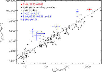
The correlation between measured gas and SFR densities for SMM J2135 compared to samples of local star-forming galaxies and ULIRGS from Kennicutt (1998) and high-redshift, as derived from 12CO(1–0). The dashed line is the best-fitting power law to local data with ΣSF∝Σ1.27gas (Genzel et al. 2010). We see that the star formation within SMM J2135 is consistent with this relation assuming rgas=rSF = 1 kpc. SMM J02399−0136 is taken from Ivison et al. (2010a), GN20 from Carilli et al. (2010) and the BzKs from Aravena et al. (2010), which are unresolved in 12CO(1–0). Hence, the arrows represent the lower limits in the measured gas density.
Although we do not have spatially resolved spectroscopy to probe the gas properties on ∼100 pc scales, we can ask where the individual star-forming regions would lie if they too followed the Kennicutt–Schmidt relation. Assuming that 80 per cent of the bolometric luminosity arises in these clumps, and that each clump has a radius of rSF=rgas∼ 100 pc, then the inferred gas density would be n∼ 3 × 105 cm-2, which is substantially higher than that inferred from the PDR and LVG modelling of the dense gas tracers (n∼ 103.5−4.5 cm−2). However, taking the remaining 20 per cent of the bolometric luminosity with a radius of 1 kpc (and assuming the gas lies in an extended disc), the density is n∼ (0.2–1) × 104 cm2 (with the main uncertainty being the disc thickness). Thus, although this calculation should be considered crude, the results are consistent with a model in which the submillimetre emission predominantly traces the star-forming clumps on ∼100 pc scales, but these clumps are simply embedded in a much more extended structure which dominates the 12CO emission. These results may also imply a break-down of the Kennicutt–Schmidt relation on scales of individual GMCs (<100 pc, see also Onodera et al. 2010), although clearly high-resolution millimetre observations would accurately constrain their sizes, which is a fundamental step in understanding the conditions within the ISM of high-redshift galaxies (P. Cox et al. in preparation).
4 CONCLUSIONS
We have presented detections of a number of rest-frame, far-IR and submillimetre molecular and atomic emission lines in the spectrum of the lensed submillimetre galaxy SMM J2135. We have used these lines to construct the 12CO SLED up to Jupper = 10 and analysed this and the other species, including the HCN(3–2) and [C i] fine structure lines, to investigate the physical conditions within the ISM in this galaxy. Our main results are:
The 12CO SLED resembles that of local starburst galaxies. An LVG analysis of the 12CO SLED shows at least two phases with temperatures T∼ 25 and 60 K.
The dust SED is best fitted by a model in which the galaxy comprises an extended component with radius ∼1–2 kpc with Td∼ 30 K and four high-density, star-forming regions with sizes of the order of r∼ 200 pc and Td∼ 60 K. These characteristics are roughly consistent with the rest-frame ∼250-μm morphology of the system as seen by the SMA and the two components may link to the phases identified from the 12CO SLED. At Jupper = 1–0, the cooler, diffuse phase appears to comprise 50 per cent of the molecular gas. We also derive a carbon mass of MC I = (9.1 ± 0.2) × 106 M⊙ and hence a carbon abundance of ∼4 × 10⁻⁵ which is slightly above the Galactic value. LVG modelling suggests that the dense, star-forming regions have abundances similar to that seen in the Milky Way, whilst the extended diffuse gas has lower metallicity (or a higher cosmic-ray flux).
Using the 12CO emission and assuming α = 0.8 we estimate the total molecular gas mass from the 12CO(1–0) emission as M(H2) = (1.4 ± 0.1) × 1010 M⊙. Comparing this with that derived from Jupper≥ 3 transitions, assuming thermalized gas, shows that these predicted gas masses are a factor of 1.5–3.6 times too low, indicative of multiple gas phases, as seen in local starbursts. However, our LVG analysis indicates a higher gas mass, M(H2) ∼ 4 × 10¹⁰ M⊙, yielding an effective CO-to-H2 conversion factor of α∼ 2.0. If these conditions are relevant in the wider SMG population, then this suggests that previous, Jupper≥ 3 12CO observations of SMGs may have underestimated the molecular gas content of SMGs by at least a factor of ∼2–5 times (see also Ivison et al. 2010a; Harris et al. 2010).
Within SMM J2135, we detect the HCN(3–2) emission at the 3σ level and use this to estimate a dense gas mass of Mdense(H2) =αHCNL′HCN < 4.5 × 10¹⁰ M⊙, assuming αHCN = 10 (Gao & Solomon 2004). Within the uncertainties in αHCN, this is consistent with the gas mass derived from 12CO, indicating that HCN may be a promising route to constraining the dense gas masses of high-redshift galaxies in the future (Gao et al. 2007), particularly if two or more HCN lines are measured. We also find that the HCN/FIR ratio is consistent with that of local ULIRGs and star-forming galaxies with no evidence for AGN contribution to the FIR luminosity.
We use the atomic fine-structure and molecular line ratios to investigate the excitation conditions within the ISM and find that they are similar to those found in local starbursts and ULIRGs. Using a grid of PDR models, we show that the molecular gas in SMM J2135 is exposed to a UV radiation field which is ∼1000 times more intense than that of the Milky Way, and has a density of n∼ 104 cm−3, both characteristic of the central regions of a typical starburst galaxy. Thus, the inferred density and far-UV radiation field strength of the ISM appear similar to those seen in local ULIRGs consistent with the interpretation of SMGs as the high-redshift analogues of these merger-driven starbursts. However, the spatial extent and mass of the gas reservoir (and spatial extent of the star formation) is larger than typically found in local ULIRGs.
We find that the 12CO emission shows multiple kinematic components and we decompose the SLEDs into three kinematic components to investigate the excitation variations within the system. We find tentative evidence of temperature variation between the kinematic components, although we defer a detailed discussion of the kinematics to a future paper (P. Cox et al., in preparation).
Using a number of approaches, we have derived estimates for the effective size of the gas reservoir within this system. All of our estimates are larger than the size of the clumps detected in the 870-μm map from SMA, implying that the gas traces a more extended structure. Overall, our modelling of the 12CO SLED supports the presence of two phases in the ISM, with one phase associated with ∼solar metallicity star-forming clumps with >100 pc sizes, embedded in a low metallicity (or high cosmic-ray flux), extended component with a characteristic size of ∼1 kpc. However, even the ‘extended’ component has a much higher gas density than typically observed in local starbursts, such as M 82 (although a similar density to local ULIRGs, such as Arp 220) and is exposed to a UV radiation field, which is ∼1000 times more intense than the Milky Way (Gerin & Phillips 1998).
Assuming that the molecular gas is evenly distributed, we show that the integrated properties of the galaxy follow the Kennicutt–Schmidt relation. We also test where the individual star-forming regions would lie, if they too followed the Kennicutt–Schmidt relation, and we show that on ∼100 pc scales, the gas density would be ∼30 times higher than that inferred from the LVG or PDR analysis. However, the properties of the diffuse gas disc suggest a characteristic density n∼ (0.2–1) × 104 cm2, which is comparable to that inferred from the LVG and PDR models. These results are consistent with a model in which the submillimetre emission predominantly traces the dense cores of the star-forming regions, but that these clumps are simply embedded in a much more extended and diffuse structure which dominates the gas emission. These results may also imply a break-down of the Kennicutt–Schmidt relation on scales of individual GMCs (e.g. <100 pc), although clearly only high-resolution millimetre observations will accurately constrain their sizes.
These results show that it is possible to unravel the complex ISM physics within starburst galaxies at high redshift at a level of detail which, until recently has only been possible in the z < 0.1 Universe. Our observations provide an unique window into the physics of star formation at z∼ 2 with an S/N that would otherwise require the increased light grasp of the next-generation facilities. Indeed this source provides insight into the science that will be routinely possible once ALMA reaches full science operations.
ALRD acknowledges an STFC studentship, AMS gratefully acknowledges a Sir Norman Lockyer Royal Astronomical Society Fellowship, IRS acknowledges support from STFC. We are very grateful to Padeli Papadopoulos for extensive disccusion and comments on this manuscript. We also thank Estelle Bayet, Carsten Kramer, Rowin Meijerink, Serena Viti, Paul van der Werf and Chris Wilson for a number of useful discussions. We thank the anonymous referee for useful comments which added to the clarity and content of this paper. The observations in this paper were carried out with the IRAM 30 m and the Plateau de Bure Interferometer. IRAM is supported by INSU/CNRS (France), MPG (Germany) and IGN (Spain). We also thank the ESO Director for generously granting DDT observations with the SHFI as part of program 283.A-5014 which is based on data acquired with the Atacama Pathfinder Experiment (APEX). APEX is a collaboration between the Max-Planck-Institut fur Radioastronomie, the European Southern Observatory and the Onsala Space Observatory. The SMA is a joint project between the Smithsonian Astrophysical Observatory and the Academia Sinica Institute of Astronomy and Astrophysics and is funded by the Smithsonian Institution and the Academia Sinica. Zpectrometer observations were taken as part of program 09A-040. Zpectrometer is supported by National Science Foundation grants AST-0503946 and AST-070865 and by the National Radio Astronomy Observatory. The National Radio Astronomy Observatory is a facility of the National Science Foundation operated under cooperative agreement by Associated Universities, Inc.
REFERENCES
