


Abstract
An analysis of large-area CO J= 3–2 maps from the James Clerk Maxwell Telescope for 12 nearby spiral galaxies reveals low velocity dispersions in the molecular component of the interstellar medium. The three lowest luminosity galaxies show a relatively flat velocity dispersion as a function of radius while the remaining nine galaxies show a central peak with a radial fall-off within 0.2–0.4r25. Correcting for the average contribution due to the internal velocity dispersions of a population of giant molecular clouds, the average cloud–cloud velocity dispersion across the galactic discs is 6.1 ± 1.0 km s−1 (standard deviation of 2.9 km s−1), in reasonable agreement with previous measurements for the Galaxy and M33. The cloud–cloud velocity dispersion derived from the CO data is on average two times smaller than the H i velocity dispersion measured in the same galaxies. The low cloud–cloud velocity dispersion implies that the molecular gas is the critical component determining the stability of the galactic disc against gravitational collapse, especially in those regions of the disc which are H2 dominated. The cloud–cloud velocity dispersion shows a significant positive correlation with both the far-infrared luminosity, which traces the star formation activity, and the K-band absolute magnitude, which traces the total stellar mass. For three galaxies in the Virgo cluster, smoothing the data to a resolution of 4.5 kpc (to match the typical resolution of high-redshift CO observations) increases the measured velocity dispersion by roughly a factor of 2, comparable to the dispersion measured recently in a normal galaxy at z= 1. This comparison suggests that the mass and star formation rate surface densities may be similar in galaxies from z= 0 to 1 and that the high star formation rates seen at z= 1 may be partly due to the presence of physically larger molecular gas discs.
1 INTRODUCTION
The vertical structure of the interstellar medium (ISM) is determined by a delicate balance between gravity and pressure. The concentration of mass in the stellar disc drags the gas into a thin disc whose vertical scaleheight is controlled by the velocity dispersion. The velocity dispersion of the gas is also an important parameter for star formation laws based on the Toomre Q criterion (Toomre 1964; Kennicutt 1989). The atomic phase of the ISM has been well studied and interpreted, most recently by Tamburro et al. (2009, see below). However, the velocity dispersion of the star-forming molecular gas is much less well understood, although the available data are consistent with a significantly thinner and dynamically colder molecular disc (Stark & Brand 1989; Wilson & Scoville 1990; Combes & Becquaert 1997).
Determining the velocity dispersion of the molecular gas in the Galaxy is complicated by our location within the plane of the disc and the difficulty in removing the effects of streaming motions associated with spiral arms. Nearby, relatively face-on galaxies are better targets, provided sufficient sensitivity and spectral and spatial resolution can be achieved. However, an additional complicating factor in any analysis is the fact that the observed velocity dispersions are not significantly larger than the internal velocity dispersion of an individual giant molecular cloud (GMC). For example, Solomon et al. (1987) measure internal velocity dispersions ranging from 1 to 8 km s−1 and a relation between internal velocity dispersion and cloud mass that goes as M = 2000 σ4v. Certainly, the net effect of the internal velocity dispersion of a population of GMCs in the beam needs to be considered in an analysis of the cloud–cloud velocity dispersion of nearby, near face-on galaxies.
For our own Galaxy, Clemens (1985) obtained a one-dimensional cloud–cloud velocity dispersion of 3.0 km s−1, significantly smaller than the value of 7–9 km s−1 obtained by Stark (1984). Stark & Brand (1989) argued that the velocity dispersion measured by Clemens (1985) is actually the internal velocity dispersion of individual clouds and obtained a cloud–cloud velocity dispersion of 7.8 ± 0.6 km s−1 for clouds within 3 kpc of the Sun. Although this measurement includes small-scale streaming motions, they argued that the true value is only 20 per cent smaller when the streaming motions are removed (Stark & Brand 1989). More recently, Stark & Lee (2005, 2006) have rederived the scaleheight of the molecular gas to be 35 pc for clouds less massive than 2 × 10⁵ M⊙ and only 20 pc for clouds more massive than this limit. This scaleheight of 20 pc implies a one-dimensional cloud–cloud velocity dispersion of just 4 km s−1 for the more massive molecular clouds. Combes & Becquaert (1997) pointed out that, given the observed scaleheights of H i and CO in the Galaxy and a velocity dispersion of 9 km s−1 in the atomic gas, we would expect a cloud–cloud velocity dispersion of only 2.4 km s−1 in the molecular gas, a value which is significantly smaller than any of the measurements.
There are relatively few measurements of the velocity dispersion of the molecular gas in other galaxies. Wilson & Scoville (1990) used a combination of interferometric observations of individual GMCs with single-dish observations of M33 to measure a cloud–cloud velocity dispersion of 5 ± 1 km s−1. Combes & Becquaert (1997) observed NGC 628 and 3938 using the CO J = 1–0 and J = 2–1 lines and observed velocity dispersions of 6 and 8.5 km s−1, respectively. They used Gaussian fits to the observed linewidths and corrected for saturation effects (García-Burillo, Combes & Gerin 1993). Walsh et al. (2002) made CO J = 1–0 and J = 3–2 observations of NGC 6946 and measured velocity dispersions from second moment maps of 8.9 ± 2.2 and 6.0 ± 1.6 km s−1 in the two lines. Neither of these two studies (Combes & Becquaert 1997; Walsh et al. 2002) attempted to correct for the internal velocity dispersion of individual GMCs, and so these measurements are upper limits to the cloud–cloud velocity dispersion.
There have been a number of theoretical attempts to model the cloud–cloud velocity dispersion in the Galaxy. Jog & Ostriker (1988) propose that cloud–cloud gravitational scattering in a differentially rotating galactic disc acts to increase the random kinetic energy of the cloud population. In this model, inelastic collisions between clouds act as an energy sink, resulting in an equilibrium value for the one-dimensional velocity dispersion of 5–7 km s−1. Gammie, Ostriker & Jog (1991) extended this work using both analytical and numerical analyses and obtained a value of 5 km s−1 for the two-dimensional velocity dispersion in the plane of the disc. Thomasson, Donner & Elmegreen (1991) performed N-body simulations of clouds and stars which include inelastic cloud collisions but not close 2-body gravitational encounters. They found typical velocity dispersions of 3 km s−1 which increase in galaxies with stronger spiral structure. More recently, Tasker & Tan (2009) have developed a three-dimensional model including ISM cooling to 300 K with a resolution of 8 pc and found typical velocity dispersions of 10 km s−1 for a model of the Milky Way.
Although there have been relatively few measurements of the velocity dispersion in the molecular gas in galaxies, the velocity dispersion of the atomic gas has been well studied (see Tamburro et al. 2009, and references therein). Most recently, the HI Nearby Galaxy Survey (THINGS) (Walter et al. 2008) has produced high-resolution H i maps of 34 spiral and irregular galaxies with distances less than 11 Mpc. The typical velocity dispersion in the atomic gas at radii between r25/2 and r25 is 11 ± 3 km s−1 for galaxies with inclinations less than 60° (Leroy et al. 2008). Tamburro et al. (2009) found an H i linewidth that falls off systematically with radius which they link to the energy provided by supernovae linked to recent star formation. They also found a characteristic H i velocity dispersion of 10 ± 2 km s−1 at r25, which often marks the extent of significant star formation in the disc.
In this paper, we present measurements of the velocity dispersion for the molecular component of the ISM using data from the James Clerk Maxwell Telescope (JCMT) Nearby Galaxies Legacy Survey (NGLS) as well as a follow-up programme on H i-rich spiral galaxies in the Virgo Cluster. We use new, wide-area observations of the CO J = 3–2 emission for 12 large spiral galaxies with inclinations of <60° and distances of <17 Mpc. We discuss the observations, data reduction and analysis methods used in Section 2. A more detailed comparison with the results of Combes & Becquaert (1997) is given in Appendix A. In Section 3, we discuss the observed values of the velocity dispersion of the CO J = 3–2 transition and the correction factor necessary due to the non-trivial internal velocity dispersion of individual GMCs. The potential need to correct for a non-isotropic velocity dispersion in galaxies with inclinations larger than about 30° is discussed in Appendix B. In Section 4, we compare our results with recent observations of the velocity dispersion of the atomic gas component from the THINGS survey (Walter et al. 2008), investigate correlations of the velocity dispersion of the molecular gas with global galaxy properties such as mass and star formation rate, discuss the implications for understanding disc stability in galaxies and compare our data with recent observations of spiral galaxies at z = 1. We give our conclusions in Section 5.
2 OBSERVATIONS AND DATA PROCESSING
2.1 JCMT CO J = 3–2 data
The CO J = 3–2 observations were obtained as part of the JCMT NGLS,1 which is observing an H i flux-limited sample of 155 galaxies within 25 Mpc (Wilson et al. 2009). The angular resolution of the JCMT at this frequency is 14.5 arcsec, which corresponds to a linear resolution ranging from 0.2 to 1.2 kpc for the galaxies in our sample. From the large (D25 > 4 arcmin) spiral galaxies observed by the NGLS, we selected nine galaxies with inclinations smaller than 60° to study the velocity dispersion. Seven additional large galaxies from the NGLS with low inclinations (IC 2574, UGC 04305, NGC 3031, 3351, 4450, 4579 and 4725) did not have sufficiently strong or extended detections in CO J = 3–2 to be useful for this analysis. To this sample, we added three spiral galaxies in the Virgo Cluster (NGC 4303, 4501 and 4535) which are not part of the NGLS survey but which have been observed in a similar manner. (A fourth Virgo Cluster galaxy, NGC 4548, did not have a strong enough detection to be useful here.) These galaxies were observed as part of a follow-up programme to the NGLS (JCMT proposal M09AC05, PI C. Wilson) to obtain CO J = 3–2 observations to complete the sample of Virgo spiral galaxies with H i fluxes of >6.3 Jy km s−1. The data for these three galaxies were obtained between 2009 February 14 and 2009 May 26.
Relevant properties of the 12 galaxies are given in Table 1. All 12 galaxies were observed in raster mapping mode to cover a rectangular area corresponding to D25/2 with a 1σ sensitivity of better than 19 mK (T*A) at a spectral resolution of 20 km s−1. We used the 16-pixel array receiver HARP-B (Buckle et al. 2009) with the ACSIS correlator configured to have a bandwidth of 1 GHz and a resolution of 0.488 MHz (0.43 km s−1 at the frequency of the CO J = 3–2 transition). The combination of uniquely high velocity resolution and large mapping area is critical for accurate measurements of the velocity dispersion in the molecular ISM.
Galaxy properties and velocity dispersions.
| Galaxy | Vhel (km s−1) | Typea | Da25 (arcmin) | ia (°) | PAb (°) | K(tot)c (mag) | log LdFIR (L⊙) | Distancee (Mpc) | σobsf (km s−1) | σc-cg (km s−1) | σH Ih (km s−1) |
| NGC 628 | 648 | SA(s)c | 10.5 | 7 | 20 | 6.84 | 9.55 | 7.3 | 4.1 ± 2.5 | 3.5 ± 0.1 | 12 |
| NGC 2403 | 121 | SAB(s)cd | 21.9 | 56 | 124 | 6.19 | 9.10 | 3.2 | 5.2 ± 4.9 | 3.9 ± 0.2 | 14 |
| NGC 3184 | 574 | SAB(rs)cd | 7.4 | 16 | 179 | 7.78 | 9.69 | 11.1 | 6.8 ± 5.9 | 5.8 ± 0.4 | 13 |
| NGC 3938 | 829 | SA(s)c | 5.4 | 25 | 52 | 7.81 | 9.72 | 14.2 | 4.4 ± 2.9 | 2.7 ± 0.3 | 10i |
| NGC 4254 | 2412 | SA(s)c | 5.4 | 29 | 56 | 6.93 | 10.62 | 16.7 | 9.2 ± 4.5 | 8.5 ± 0.3 | – |
| NGC 4303 | 1577 | SAB(rs)bc | 6.5 | 17 | 318 | 6.84 | 10.59 | 16.7 | 8.0 ± 4.2 | 7.2 ± 0.2 | – |
| NGC 4321 | 1599 | SAB(s)bc | 7.6 | 32 | 143 | 6.59 | 10.47 | 16.7 | 12 ± 11 | 11.1 ± 0.6 | – |
| NGC 4501 | 2213 | SA(rs)b | 6.9 | 58 | 140 | 6.27 | 10.41 | 16.7 | 20 ± 15 | 20 ± 2 | – |
| NGC 4535 | 1972 | SAB(s)c | 7.1 | 41 | 0 | 7.38 | 10.12 | 16.7 | 5.1 ± 4.4 | 3.7 ± 0.4 | – |
| NGC 4736 | 295 | (R)SA(r)ab | 11.2 | 36 | 296 | 5.11 | 9.79 | 5.2 | 12 ± 9 | 11.9 ± 0.7 | 25 |
| NGC 4826 | 390 | (R)SA(rs)ab | 10.0 | 57 | 121 | 5.33 | 9.85 | 7.5 | 14 ± 11 | 13 ± 2 | 60 |
| NGC 5055 | 495 | SA(rs)bc | 12.6 | 59 | 102 | 5.61 | 10.30 | 8.0 | 9.4 ± 6.6 | 8.7 ± 0.3 | 24 |
b Position angle used for radial averages. NGC 628, 3184: Tamburro et al. (2008); NGC 2403, 4736, 4826, 5055: de Blok et al. (2008); NGC 3938: Paturel et al. (2000); NGC 4254, 4303, 4501, 4535: (Cayatte et al. 1990); NGC 4321: Knapen et al. (1993).
cK-band total apparent magnitude from Jarrett et al. (2003).
d From Sanders et al. (2003) adjusted for the distances adopted here.
e NGC 628: Karachentsev et al. (2004); NGC 2403: Freedman et al. (2001); NGC3184: Leonard et al. (2002); NGC 3938, 5055: distance calculated using the Hubble flow distance with velocity corrected for Virgo infall (Mould et al. 2000) and H0 = 73 km s−1 Mpc−1; Virgo Cluster: Mei et al. (2007); NGC 4736, 4826: Tonry et al. (2001).
f Observed CO J = 3–2 velocity dispersion and standard deviation. Regions of high velocity dispersion in the outer portions of the disc were masked before calculating the velocity dispersion (see the text). Excludes a 5.3-kpc diameter region in the centre of each Virgo galaxy (9 pixels), NGC 3938 (11 pixels) and NGC 5055 (19 pixels). All pixels are included for NGC 628, 2403 and 3184. For NGC 4736 and 4826, a 9-pixel region is excluded to give an upper limit to the outer disc velocity dispersion (see the text). Note that the uncertainty in the mean for σobs is the same as for σc-c.
g Mean cloud–cloud velocity dispersion and the uncertainty in the mean corrected for the contribution from the internal velocity dispersion of individual giant molecular clouds (see the text). Note that the uncertainty in the mean is calculated from the standard deviation given in the previous column by dividing by  , where N is the number of measurements for a given galaxy.
h H i velocity dispersion measured from naturally weighted maps from Walter et al. (2008) over the same area as the CO measurement.
i From van der Kruit & Shostak (1982).
Galaxy properties and velocity dispersions.
| Galaxy | Vhel (km s−1) | Typea | Da25 (arcmin) | ia (°) | PAb (°) | K(tot)c (mag) | log LdFIR (L⊙) | Distancee (Mpc) | σobsf (km s−1) | σc-cg (km s−1) | σH Ih (km s−1) |
| NGC 628 | 648 | SA(s)c | 10.5 | 7 | 20 | 6.84 | 9.55 | 7.3 | 4.1 ± 2.5 | 3.5 ± 0.1 | 12 |
| NGC 2403 | 121 | SAB(s)cd | 21.9 | 56 | 124 | 6.19 | 9.10 | 3.2 | 5.2 ± 4.9 | 3.9 ± 0.2 | 14 |
| NGC 3184 | 574 | SAB(rs)cd | 7.4 | 16 | 179 | 7.78 | 9.69 | 11.1 | 6.8 ± 5.9 | 5.8 ± 0.4 | 13 |
| NGC 3938 | 829 | SA(s)c | 5.4 | 25 | 52 | 7.81 | 9.72 | 14.2 | 4.4 ± 2.9 | 2.7 ± 0.3 | 10i |
| NGC 4254 | 2412 | SA(s)c | 5.4 | 29 | 56 | 6.93 | 10.62 | 16.7 | 9.2 ± 4.5 | 8.5 ± 0.3 | – |
| NGC 4303 | 1577 | SAB(rs)bc | 6.5 | 17 | 318 | 6.84 | 10.59 | 16.7 | 8.0 ± 4.2 | 7.2 ± 0.2 | – |
| NGC 4321 | 1599 | SAB(s)bc | 7.6 | 32 | 143 | 6.59 | 10.47 | 16.7 | 12 ± 11 | 11.1 ± 0.6 | – |
| NGC 4501 | 2213 | SA(rs)b | 6.9 | 58 | 140 | 6.27 | 10.41 | 16.7 | 20 ± 15 | 20 ± 2 | – |
| NGC 4535 | 1972 | SAB(s)c | 7.1 | 41 | 0 | 7.38 | 10.12 | 16.7 | 5.1 ± 4.4 | 3.7 ± 0.4 | – |
| NGC 4736 | 295 | (R)SA(r)ab | 11.2 | 36 | 296 | 5.11 | 9.79 | 5.2 | 12 ± 9 | 11.9 ± 0.7 | 25 |
| NGC 4826 | 390 | (R)SA(rs)ab | 10.0 | 57 | 121 | 5.33 | 9.85 | 7.5 | 14 ± 11 | 13 ± 2 | 60 |
| NGC 5055 | 495 | SA(rs)bc | 12.6 | 59 | 102 | 5.61 | 10.30 | 8.0 | 9.4 ± 6.6 | 8.7 ± 0.3 | 24 |
| Galaxy | Vhel (km s−1) | Typea | Da25 (arcmin) | ia (°) | PAb (°) | K(tot)c (mag) | log LdFIR (L⊙) | Distancee (Mpc) | σobsf (km s−1) | σc-cg (km s−1) | σH Ih (km s−1) |
| NGC 628 | 648 | SA(s)c | 10.5 | 7 | 20 | 6.84 | 9.55 | 7.3 | 4.1 ± 2.5 | 3.5 ± 0.1 | 12 |
| NGC 2403 | 121 | SAB(s)cd | 21.9 | 56 | 124 | 6.19 | 9.10 | 3.2 | 5.2 ± 4.9 | 3.9 ± 0.2 | 14 |
| NGC 3184 | 574 | SAB(rs)cd | 7.4 | 16 | 179 | 7.78 | 9.69 | 11.1 | 6.8 ± 5.9 | 5.8 ± 0.4 | 13 |
| NGC 3938 | 829 | SA(s)c | 5.4 | 25 | 52 | 7.81 | 9.72 | 14.2 | 4.4 ± 2.9 | 2.7 ± 0.3 | 10i |
| NGC 4254 | 2412 | SA(s)c | 5.4 | 29 | 56 | 6.93 | 10.62 | 16.7 | 9.2 ± 4.5 | 8.5 ± 0.3 | – |
| NGC 4303 | 1577 | SAB(rs)bc | 6.5 | 17 | 318 | 6.84 | 10.59 | 16.7 | 8.0 ± 4.2 | 7.2 ± 0.2 | – |
| NGC 4321 | 1599 | SAB(s)bc | 7.6 | 32 | 143 | 6.59 | 10.47 | 16.7 | 12 ± 11 | 11.1 ± 0.6 | – |
| NGC 4501 | 2213 | SA(rs)b | 6.9 | 58 | 140 | 6.27 | 10.41 | 16.7 | 20 ± 15 | 20 ± 2 | – |
| NGC 4535 | 1972 | SAB(s)c | 7.1 | 41 | 0 | 7.38 | 10.12 | 16.7 | 5.1 ± 4.4 | 3.7 ± 0.4 | – |
| NGC 4736 | 295 | (R)SA(r)ab | 11.2 | 36 | 296 | 5.11 | 9.79 | 5.2 | 12 ± 9 | 11.9 ± 0.7 | 25 |
| NGC 4826 | 390 | (R)SA(rs)ab | 10.0 | 57 | 121 | 5.33 | 9.85 | 7.5 | 14 ± 11 | 13 ± 2 | 60 |
| NGC 5055 | 495 | SA(rs)bc | 12.6 | 59 | 102 | 5.61 | 10.30 | 8.0 | 9.4 ± 6.6 | 8.7 ± 0.3 | 24 |
b Position angle used for radial averages. NGC 628, 3184: Tamburro et al. (2008); NGC 2403, 4736, 4826, 5055: de Blok et al. (2008); NGC 3938: Paturel et al. (2000); NGC 4254, 4303, 4501, 4535: (Cayatte et al. 1990); NGC 4321: Knapen et al. (1993).
cK-band total apparent magnitude from Jarrett et al. (2003).
d From Sanders et al. (2003) adjusted for the distances adopted here.
e NGC 628: Karachentsev et al. (2004); NGC 2403: Freedman et al. (2001); NGC3184: Leonard et al. (2002); NGC 3938, 5055: distance calculated using the Hubble flow distance with velocity corrected for Virgo infall (Mould et al. 2000) and H0 = 73 km s−1 Mpc−1; Virgo Cluster: Mei et al. (2007); NGC 4736, 4826: Tonry et al. (2001).
f Observed CO J = 3–2 velocity dispersion and standard deviation. Regions of high velocity dispersion in the outer portions of the disc were masked before calculating the velocity dispersion (see the text). Excludes a 5.3-kpc diameter region in the centre of each Virgo galaxy (9 pixels), NGC 3938 (11 pixels) and NGC 5055 (19 pixels). All pixels are included for NGC 628, 2403 and 3184. For NGC 4736 and 4826, a 9-pixel region is excluded to give an upper limit to the outer disc velocity dispersion (see the text). Note that the uncertainty in the mean for σobs is the same as for σc-c.
g Mean cloud–cloud velocity dispersion and the uncertainty in the mean corrected for the contribution from the internal velocity dispersion of individual giant molecular clouds (see the text). Note that the uncertainty in the mean is calculated from the standard deviation given in the previous column by dividing by , where N is the number of measurements for a given galaxy.
h H i velocity dispersion measured from naturally weighted maps from Walter et al. (2008) over the same area as the CO measurement.
i From van der Kruit & Shostak (1982).
Details of the reduction of the CO J = 3–2 data are given in Wilson et al. (2009) and Warren et al. (2010) and so we discuss here only the most important processing steps and those steps that differed from the previous analysis. The individual raw data files were flagged to remove data from any of the 16 individual receptors with bad baselines and then the scans were combined into a data cube using a sinc(πx)sinc(kπx) kernel as the weighting function to determine the contribution of individual receptors to each pixel in the final map. The pixel size in the maps is 7.276 arcsec. A mask was created to identify line-free regions of the data cube, and a first-order baseline was fitted to these line-free regions and subtracted from the cube.
 is the intensity-weighted mean velocity of that pixel. This method of calculating the velocity dispersion differs from that used by Combes & Becquaert (1997), who fitted Gaussian profiles to the CO lines. However, in the limit of Gaussian lines with a high signal-to-noise ratio, the values from the moment 2 maps should agree with the results from fitting a Gaussian directly to the line profiles. A more detailed comparison of our data with Combes & Becquaert (1997) is given in Appendix A. Moment 2 maps are often used to determine the velocity dispersion in the atomic gas, although this method is most reliable for simple line shapes, as warped discs and H i at large scaleheights can distort the line profiles (de Blok et al. 2008).
Because we were using a relatively low signal-to-noise ratio threshold in creating our masks, the final moment 2 maps sometimes appeared to contain spuriously high values typically in the outer portions of the map. These regions appear white in Figs 1 and 2. These values would bias the dispersions upwards if they were included in our averages. For five galaxies in our sample, NGC 4321, 628, 2403, 3184 and 4826, we applied an upper threshold to remove pixels with values that were higher than the highest value seen in the central part of the galaxy. The thresholding values used were 15 km s−1 for NGC 628, 25 km s−1 for NGC 2403 and 3184, 52 km s−1 for NGC 4321 and 85 km s−1 for NGC 4826. We also applied a threshold cut of 65 km s−1 to NGC 4501, but very high values persisted in the north-western portion of the map (see below); the velocity dispersions in Table 1 are measured in the south-east portion of the map only. For NGC 5055, we used a targeted threshold to remove the block of high values seen in the north-east portion of the map.
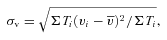
CO J = 3–2 velocity dispersion for six galaxies which are not members of the Virgo cluster. (a) NGC 628. Contour levels are 2.5, 5 and 10 km s−1 and the colour scale peak is 15 km s−1. (b) NGC 3184. Contour levels are 5, 10 and 15 km s−1 and the colour scale peak is 25 km s−1. (c) NGC 3938. Contour levels and colour scale are the same as for NGC 3184. (d) NGC 4736. Contour levels are 10, 20, … , 60 km s−1 and the colour scale peak is 85 km s−1. (e) NGC 4826. Contour levels and colour scale are the same as for NGC 4736. (f) NGC 5055. Contour levels and colour scale are the same as for NGC 4736.
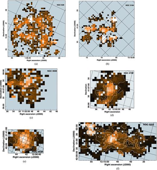
CO J = 3–2 velocity dispersion for five galaxies which are members of the Virgo cluster and NGC 2403, which is the closest galaxy in our sample. Colour scale runs from 0 (black) to 50 km s−1 (white) and contour levels are 10, 20, 30, 40 and 50 km s−1 unless otherwise noted. (a) NGC 4254. (b) NGC 4303. (c) NGC 4321. (d) NGC 4501. Contour levels are 10, 20, … , 60 km s−1 and the colour scale peak is 65 km s−1. (e) NGC 4535. (f) NGC 2403. Contour levels are 5, 10 and 15 km s−1 and the colour scale peak is 25 km s−1.
2.2 H i data from THINGS
For the six galaxies (NGC 628, 2403, 3184, 4736, 4826 and 5055) that are in common between our sample and the THINGS sample (Walter et al. 2008), we can compare the velocity dispersions in the atomic and molecular gas directly. The moment 2 maps for the THINGS sample were produced using a slightly different masking technique (Walter et al. 2008) than the one we adopted for our CO analysis. In the THINGS processing, the data are first smoothed to a resolution of 30 arcsec. A mask is then made keeping only those pixels and velocity channels (width of either 2.6 or 5.2 km s−1) where the emission exceeds 2σ in three adjacent velocity channels. We used the natural weighted maps of the H i velocity dispersion and measured the dispersion over the same region in which the CO dispersions have been measured. These velocity dispersions are also given in Table 1. Note that these H i dispersions are somewhat larger than the typical value of 11 ± 3 km s−1 given in Leroy et al. (2008) because they are measured in the inner rather than the outer discs of the galaxies.
3 VELOCITY DISPERSIONS IN THE MOLECULAR GAS DISC
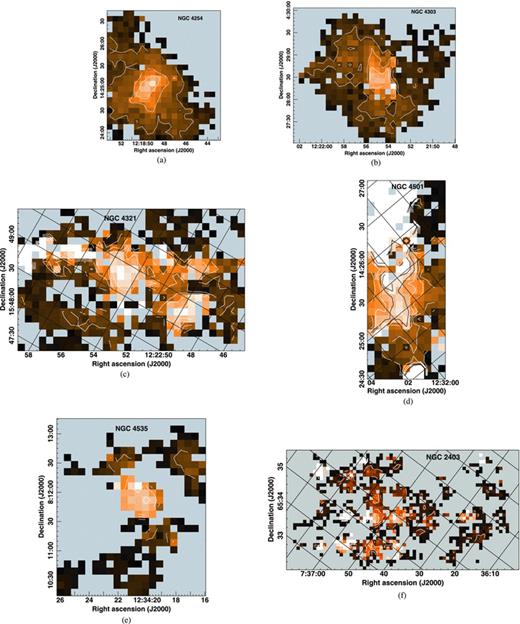
The observed CO velocity dispersion maps are shown in Figs 1 and 2. Figs 3 and 4 show the observed velocity dispersion as a function of radius for the 12 galaxies in our sample. Beam smearing is expected to have an effect only on the measured velocity dispersions for the central pixel in each plot. Three of the galaxies (NGC 628, 2403 and 3184) show very flat profiles as a function of radius. These late-type spirals are also the least luminous and so presumably are also the least massive galaxies in our sample. The remaining nine galaxies show a central peak in the velocity dispersion extending to 0.2–0.4r25. We attribute part of this increase to the effects of a steeply rising rotation curve at our relatively low (0.2–1.2 kpc) spatial resolution in these galaxies. Thus, for these galaxies, we measure the average velocity dispersion in the outer disc excluding a central circular region. The exclusion aperture was chosen by examining the individual velocity dispersion maps to identify the smallest aperture that would exclude the region of most obviously enhanced dispersion. We found that a diameter of 5.3 kpc (9 pixels or 65 arcsec at the distance of Virgo) worked well for all five galaxies in the Virgo cluster and that a similar physical region was appropriate for the other galaxies in our sample. However, the maps of NGC 4736 and 4826 contain no data at larger radii, and so for these two galaxies we quote disc velocity dispersions excluding only a central 9-pixel diameter region. The disc velocity dispersions of these two galaxies are likely biased to be somewhat higher than those of the other galaxies in our sample, and thus we do not include them in calculating the average outer disc velocity dispersion.
Observed CO J = 3–2 velocity dispersion as a function of radius normalized by r25. These velocity dispersions have not been corrected for any contribution from the internal velocity dispersion of individual GMCs (see the text). Where appropriate, the central region excluded from calculating the disc-averaged velocity dispersion is indicated by the dashed line.
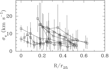
Observed CO J = 3–2 velocity dispersion as a function of radius normalized by r25, showing nine galaxies on a single plot. Data points with r < 2.65 kpc are not plotted for the six galaxies with central peaks in the velocity dispersion.
The average observed velocity dispersions in the molecular gas measured for the 12 galaxies in our sample are given in Table 1. These velocity dispersions are consistent with previous measurements for the Milky Way (Stark & Brand 1989), M33 (Wilson & Scoville 1990) and other nearby galaxies (Combes & Becquaert 1997; Walsh et al. 2002). The observed velocity dispersion in the molecular gas disc ranges from a low of 4.1 km s−1 in NGC 628 to a high of 20.1 km s−1 in NGC 4501. We exclude NGC 4736 and 4826 from our averages because we can only trace the velocity dispersions in the inner region where the profile is still rising steeply. We further exclude NGC 4501 because its very high velocity dispersion and evidence for double-peaked line profiles in the north-west portion of the disc suggest that the molecular gas has been affected by the same ram pressure effects seen in H i (Vollmer et al. 2008). The average observed value for the remaining nine galaxies is 7.1 ± 0.9 km s−1 (standard deviation of 2.6 km s−1), 50 per cent smaller than the average of 11 ± 3 km s−1 measured for the atomic gas in the outer discs of spiral galaxies (Leroy et al. 2008). If we compare the atomic and molecular velocity dispersions in the same region of the disc (Table 1), the observed velocity dispersion in the molecular gas is on average approximately two times smaller than the dispersion in the atomic gas.
3.1 The effect of cloud internal velocity dispersions
The low values measured for the velocity dispersion, particularly for NGC 628 and 3938, lead us to consider the effect of internal velocity dispersions of individual GMCs on the observed velocity dispersion. A second complicating effect, that of an anisotropy between the vertical and in-plane motions of the GMCs, would be expected to produce a correlation of velocity dispersion with inclination, which is not seen in our data (Fig. B1). Nevertheless, we discuss the potential magnitude of this effect in Appendix B.
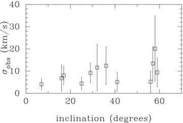
Observed CO J = 3–2 velocity dispersion as a function of the galaxy inclination angle. Error bars show the standard deviation of the observed values within an individual galaxy.
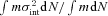
Individual GMCs have internal velocity dispersions that are substantially larger than the thermal linewidths expected for gas with physical temperatures of 10–30 K. In the study of Solomon et al. (1987), individual GMCs show internal velocity dispersions ranging from 1 to 8 km s−1. These internal velocity dispersions are obtained from an intensity-weighted measure of the dispersion in radial velocity within a single cloud and thus are directly comparable (in technique) to the intensity-weighted dispersions averaged over the galactic disc presented here. What we need is an estimate of the contribution of the internal velocity dispersions of an ensemble of GMCs with a range of masses to the observed velocity dispersion in the disc. With this value, it is easy to show that the observed velocity dispersion, σv, is given by  , where
  is the mass-weighted average internal velocity dispersion for our ensemble of clouds and σc-c is the value we are interested in measuring, that is, the cloud–cloud velocity dispersion.
 which, using the relation between σint and M given by Solomon et al. (1987) and assuming α≠ 2, reduces to
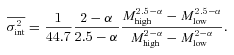
 km s−1. The exact result clearly depends on the details of the model.
Interestingly, this estimate of the average cloud internal velocity dispersion is comparable to the value of 4.1 km s−1 observed in the disc of NGC 628. The average CO J = 3–2 intensity in NGC 628 of 0.8 K km s−1 is the lowest intensity in our sample and translates into an average mass per JCMT beam of only 4 × 10⁶ M⊙. For a GMC mass function with slope α = 1.5, this surface density translates into an average of just 10 clouds with 105 < M < 106 M⊙ per beam. This calculation suggests that, although the number of massive (>105 M⊙) GMCs per beam may be subject to small-number statistics in NGC 628, their effect on the velocity dispersion should be observable on average if such large clouds are present in NGC 628. This analysis suggests that NGC 628 is likely deficient in the largest molecular clouds; if we instead limit the maximum cloud mass to 105 M⊙, then the mass-weighted average internal velocity dispersion reduces to  km s−1. The larger average integrated intensities and observed velocity dispersions suggest that the molecular cloud mass spectrum is likely to be fully populated in the remaining galaxies in our sample. Thus, in correcting the observed velocity dispersions for the effects of internal cloud velocity dispersions, we use a value for
  of 2.2 km s−1 for NGC 628 and 3.5 km s−1 for the rest of the sample. The corrected values for the cloud–cloud velocity dispersion are given in Table 1 along with the uncertainty in the mean cloud–cloud velocity dispersion for each galaxy. The uncertainty in the mean has been calculated assuming that the errors are normally distributed, so that the uncertainty in the mean is given by the standard deviation divided by
  , where N is the number of measurements for a given galaxy.
3.2 The true vertical velocity dispersion of the molecular gas
Based on the discussion in the previous section, the observed velocity dispersion includes both a contribution from the internal velocity dispersion of individual GMCs and a contribution from the cloud–cloud velocity dispersion. It is this second quantity, the cloud–cloud velocity dispersion, which is of interest for determining the molecular gas scaleheight, analysing the stability of the gas disc, etc. The small observed velocity dispersions imply that the correction for the internal velocity dispersion of the clouds is not negligible. Correcting for the average internal cloud velocity dispersion, as discussed in Section 3.1, gives measures of the cloud–cloud velocity dispersions which range from 2.7 to 19.8 km s−1. Again excluding NGC 4501, 4736 and 4826, we obtain an average value of 6.1 ± 1.0 km s−1 (standard deviation of 2.9 km s−1).
4 DISCUSSION
4.1 Molecular and atomic gas velocity dispersions
The average cloud–cloud velocity dispersion in the molecular gas in this group of spiral galaxies of 6.1 ± 1.0 km s−1 is slightly smaller than previous estimates for external galaxies which did not take the effect of internal cloud dispersion into account (Combes & Becquaert 1997; Walsh et al. 2002), but is comparable to recent measurements for the cloud–cloud dispersion of massive clouds in the Galaxy (Stark & Lee 2006) and in M33 (Wilson & Scoville 1990).
4.1.1 Effects of CO optical depth
An additional possible concern in interpreting the CO data is the high optical depth of the CO line. Since we are interested in the cloud–cloud velocity dispersion, it is important to check whether the surface density of the molecular gas is sufficiently high that shielding of one cloud by another at a similar velocity could affect our measurements. For all but one of the galaxies in our sample, the projected surface density NH is substantially smaller than the typical surface density of individual GMCs (NH = 1.5 ± 0.3 × 1022 cm−1; McKee 1989), and thus cloud–cloud shielding is unlikely to be a problem. Only in NGC 4736, where the surface density may be as high as 3 × 1022 cm−2[assuming a CO J = 3–2/J = 1–0 line ratio of 0.3 and a CO-to-H2 conversion factor of 2 × 1020 cm−2 (K km s−1)−1; Strong et al. 1988], is it possible that the clouds may shield one another to some degree. However, the actual surface density depends sensitively on the value that we assume for the CO J = 3–2/J = 1–0 line ratio; if we adopt a value of 0.6 which is more appropriate for the dense gas, rather than the value of 0.3 found in a direct comparison of CO J = 3–2 and J = 1–0 maps of NGLS galaxies (Wilson et al. 2009; Warren et al. 2010), then the projected disc-averaged column density is similar to that of individual GMCs. Thus, we conclude that we can ignore the possibility of cloud–cloud shielding in the discs of the galaxies in this sample.
4.1.2 Observed H i velocity dispersions
Combes & Becquaert (1997) showed that the molecular and atomic components in NGC 628 and 3938 had vertical velocity dispersions that are similar to each other and virtually constant with radius. As a consequence, the authors suggested that the two layers had similar scaleheights and that H i and H2 simply represent different phases of the same dynamical component. It is clear, however, from observations of our own Milky Way as well as edge-on galaxies that the molecular disc is significantly thinner than the H i disc. Our observed velocity dispersions are comparable to those found by Combes & Becquaert (1997), although we have shown that it is necessary to correct for internal velocity dispersion to determine the cloud–cloud velocity dispersion that is relevant for scaleheight determinations. For H i, on the other hand, we know that its stable phases occur in both hot diffuse gas and colder clouds (the warm neutral medium and cold neutral medium, respectively). Although discrete H i clouds are identifiable in our Galaxy (see Lockwood 2001; Stil et al. 2006), the clouds are smaller and warmer than molecular clouds. Because of the admixture of cool and warm H i components over the size scale of the beam in external galaxies, similar corrections need not be applied to the H i velocity dispersions. Also, since the H i is a diffuse collisional medium, its velocity dispersion is assumed to be isotropic (e.g. Malhotra 1995). We have therefore compared the observed H i dispersion directly with our cloud–cloud velocity dispersion derived from the CO data.
4.1.3 Comparing CO and H i velocity dispersions
The published H i velocity dispersion map for NGC 4501 (Vollmer et al. 2008) shows velocity dispersions in the range of 10–20 km s−1 across the extended disc, comparable to the cloud–cloud velocity dispersion (Table 1) over the same area. High-resolution H i data have been published for NGC 4321 (Knapen et al. 1993) and NGC 4254 (Phookun, Vogel & Mundy 1993), but the velocity dispersion maps are not presented; we could find no published high-resolution H i data for NGC 4303 and 4535. An older measurement of the H i velocity dispersion of 10 km s−1 for NGC 3938 (van der Kruit & Shostak 1982) is roughly three times larger than our derived cloud–cloud velocity dispersion.
We have compared the velocity dispersions in the molecular and atomic gas measured over the same regions for six galaxies in our sample for which maps of the atomic gas velocity dispersion are available from the THINGS sample (Walter et al. 2008). On average, the cloud–cloud velocity dispersion determined from CO data is roughly half that of the atomic gas. The exception to this trend is NGC 4826, for which the cloud–cloud velocity dispersion is a factor of 5 times smaller than the H i velocity dispersion. However, this galaxy has quite a steep radial gradient in the observed velocity dispersion (Fig. 3) and so the average disc value depends sensitively on what aperture is used. Overall, these results imply that the scaleheight of the molecular gas is roughly half that of the atomic gas. This estimate of the ratio of the scaleheights is roughly consistent with the estimate of the relative H i and CO scaleheights in the Milky Way as discussed in Combes & Becquaert (1997). We should note, however, that narrow (4–5 km s−1) H i line components have been seen in a few Local Group dwarf galaxies observed with high spatial resolution (Young & Lo 1996, 1997; de Blok & Walter 2006). These narrow lines, which may represent atomic gas cooling to form the precursors of GMCs, are typically superimposed on a broader underlying line which likely represents the overall warm neutral atomic medium.
4.2 Correlations with other global properties
The infrared luminosity is a useful tracer of the star formation activity within a galaxy (Kennicutt 1998). Enhanced star formation might be expected to increase the velocity dispersion in the ISM via stellar winds and supernova explosions. Indeed, Tamburro et al. (2009) find evidence that supernovae linked to recent star formation are important for maintaining the velocity dispersion in the atomic gas. We find a statistically significant correlation (95 per cent confidence level) of both the observed and the cloud–cloud velocity dispersion with infrared luminosity (Sanders et al. 2003) for the nine galaxies in our sample. Thus, like the atomic gas, there is some evidence for star formation activity enhancing the velocity dispersion in the dense molecular gas. We also find a statistically significant correlation (95 per cent confidence level) of both the observed and the cloud–cloud velocity dispersion with the absolute K-band and absolute B-band magnitude (Jarrett et al. 2003). Assuming the K-band magnitude traces the total stellar mass, this correlation suggests that the cloud–cloud velocity dispersion is enhanced in more massive galaxies. For all these correlations, however, it is important to keep in mind that we have compared the average velocity dispersion in the disc (excluding the central regions) with a global luminosity which would include the contribution from the central regions.
There also appears to be a dependence in our sample of the velocity dispersion on galaxy morphology. We divided our sample into early (type ab-bc) and late (type c-cd) spirals and calculated the average velocity dispersion for each sub-sample. The average observed dispersion for six late-type spirals is 5.8 ± 0.3 km s−1, while the value for three early-type spirals is 9.7 ± 0.6 km s−1. These two values differ at the 6σ level. Of course, this dependence on morphology could be tracing some other variable in our sample, such as mass or star formation activity. In fact, the average infrared luminosities differ by a factor of 3 between the early- and late-type samples, while the K-band luminosity differs by a factor of 4. Thus, it seems most likely that the dependence on morphology is driven by differences in the average star formation rates and masses between the early- and late-type samples.
4.3 Disc stability and star formation laws
The velocity dispersion of the ISM is an important parameter in understanding the stability of galactic discs against gravitational collapse. Jog & Solomon (1984a,b) showed that a rotating disc composed of two fluids with different surface densities and velocity dispersions can be unstable to perturbations even if each fluid disc is stable on its own. They also showed that a galaxy must be treated as a two-fluid system when the colder gaseous component comprises as little as 10 per cent of the total mass of the system. Treating the stellar component as a collisional fluid, they found that the critical velocity dispersion required for stability in this higher dispersion system is larger in the presence of a second cold fluid than if the stellar system is treated in isolation. Rafikov (2001) considered the case of a single fluid and multiple collisionless (stellar) components, but found that the stability conditions were quite similar in the two-fluid case whether or not the stellar component was treated as collisionless.
Yang et al. (2007) applied the approach of Rafikov (2001) to compare the location of star forming regions in the Large Magellanic Cloud with the disc stability criterion. They adopted a gas velocity dispersion of 5 km s−1, very similar to the value found in our sample of spiral galaxies. They found that there was a much better spatial correlation of star-forming regions with regions where the disc was unstable when instability was evaluated using the contribution of both the gas and the stars. Leroy et al. (2008) applied the two-collisional-fluid equation of Rafikov (2001) to a number of galaxies in the THINGS sample (Walter et al. 2008). They adopted a gas velocity dispersion of 11 km s−1 from measurements of the H i component. Similar to Yang et al. (2007), they found that the Q values were smaller when both the stars and the gas were included in the analysis; however, they found that the discs were globally stable against large-scale perturbations.
The results for the molecular velocity dispersion presented here imply that the ISM in spiral galaxies is itself a multifluid system, with the molecular gas disc being dynamically significantly colder than the atomic gas disc. Since previous analyses have found that the colder of the two components has the larger effect on the disc stability (Jog & Solomon 1984a), it seems likely that, if we were to use one phase of the ISM in our stability analysis, it should be the dynamically coldest phase, which is the molecular gas. This would be especially true for the inner regions of those spiral discs where the ISM mass is predominantly H2. The Toomre Q parameter for the combined system tends to decrease as the velocity dispersion of the coldest (gas) component decreases and as the gas mass fraction (Σgas/Σ*) increases (Jog & Solomon 1984b; Rafikov 2001). This effect suggests that the Q values derived by Leroy et al. (2008) are likely to be significantly larger than the values that would be derived if the molecular gas values for surface density and velocity dispersion were used in the analysis, a possibility that was discussed in Leroy et al. (2008) as well. It would be informative to repeat the stability analysis for the galaxies in common between our sample and the THINGS sample to see if the discs remain globally stable as judged by the Q parameter when the cloud–cloud velocity dispersion of the molecular gas is included. We plan to investigate this issue further in a future paper.
The need to treat the ISM itself as a multifluid system suggests that we may not be able to separate the discussion of the instabilities in the atomic and molecular phases. For example, we might imagine that the Q value for the atomic gas governs the formation of molecular clouds from the H i disc, while the star formation from those clouds would then be governed by the Q value for the molecular disc. However, the two-fluid analysis by Jog & Solomon (1984a) and Rafikov (2001) implies that the Q value and hence the stability properties of the atomic disc are affected by the presence of the dynamically colder molecular disc. In particular, an atomic gas disc with a stable value of Q when considered in isolation might be found to be unstable when the presence of a relatively small quantity of molecular gas is included. Of course, a complete analysis would include the properties of the stellar disc (perhaps multiple components, as in Rafikov 2001) in addition to the two fluid components of the ISM. Such an analysis is beyond the scope of this paper.
4.4 Implications for turbulent support of the ISM
The scaleheight of a gaseous component in hydrostatic equilibrium depends on both gravitational and pressure gradients. Gravitational gradients originate in the disc as well as a dark matter halo potential. The pressure will include internal thermal pressure, turbulent pressure and, if important, pressure due to cosmic rays and magnetic fields. At the radius of the Sun in the Milky Way, the magnetic and cosmic ray pressures supply about half of the total pressure and the thermal and turbulent pressures supply the remaining half (Hanasz & Lesch 2004). At the temperatures of the molecular components, turbulent pressure dominates over thermal pressure within and between clouds (e.g. Brunt 2003). In the H i, thermal pressure likely dominates in the warm neutral medium whereas both may be important for the cold neutral medium (Heiles & Troland 2003). Measured velocity dispersions can only probe the dynamical components (thermal and turbulent) and therefore can only predict the scaleheight of the gas provided that the dynamical components dominate over the magnetic and cosmic ray pressures and that the disc ISM is in pressure equilibrium.
Star formation activity is typically associated with heating sources and sources of turbulence through supernovae and stellar winds. Most of the galaxies in our sample show a radial decline in the CO velocity dispersion (Fig. 4). The velocity dispersion in H i is also a declining function of radius (Tamburro et al. 2009), although H i discs retain significant velocity dispersions outside any star-forming disc (e.g. Sellwood & Balbus 1999; Tamburro et al. 2009). Tamburro et al. (2009) found a good correlation between the kinetic energy of the H i and the star formation rate and suggested that supernovae are likely sufficient to maintain the H i velocity dispersion in regions with significant star formation. The correlation of the cloud–cloud velocity dispersion with the star formation rate as traced by the infrared luminosity suggests that star formation may also be the dominant source of turbulence in the H2-rich parts of spiral discs.
However, some galaxies do show a lack of correlation between turbulence in the atomic gas and star formation as a function of radius. (e.g. Dickey, Hanson & Helou 1990; van Zee & Bryant 1999; Petric & Rupen 2007). The three lowest luminosity galaxies in our sample show a roughly constant cloud–cloud velocity dispersion as a function of radius (see also Combes & Becquaert 1997). These results suggest that non-thermal energy input in the form of turbulence that is unrelated to star formation may be important for understanding the vertical velocity dispersions in discs. Magnetic instabilities may be the most promising source of turbulence. Parker instabilities (Parker 1966) are well known, but seem to require cosmic rays from supernovae as triggers to be most effective (Hanasz & Lesch 2000). Thus, Parker instabilities cannot account for the observed dispersions seen outside of the active star-forming disc, but could be important for the inner molecular discs where star formation is occurring. Another possibility is the Balbus–Hawley (or magnetorotational) instability (Balbus & Hawley 1991, 1998) or other instabilities related to magnetic stresses (e.g. Sellwood & Balbus 1999). Tamburro et al. (2009) suggest that a combination of thermal broadening and magnetorotational instabilities can account for the H i velocity dispersion beyond r25. Simulations of the magnetorotational instability by Piontek & Ostriker (2007) for the two-phase H i component have shown that the turbulent velocity amplitude varies as ∝n−0.77, where n is the mean density of the component. If this turbulence is dominant in both molecular and atomic gas, then the difference in velocity dispersion between the two components may simply relate to their respective densities.
4.5 Disc galaxies at high redshift
Observations of the molecular gas content in galaxies at redshifts z = 1–3 are often made using the CO J = 3–2 line, which at these redshifts falls into the standard millimetre observing windows. Most high-resolution detections of high-redshift galaxies are unusually luminous systems, such as submillimetre galaxies (Tacconi et al. 2008) or quasars (Coppin et al. 2008). Although many of these high-redshift detections appear as simple point sources at current resolution limits, there are a few systems for which we can begin to resolve the velocity structure. Even more interesting from the point of view of this paper are the observations of more normal galaxies at redshifts of 1–1.5, which are becoming available (Daddi et al. 2008, 2010; Dannerbauer et al. 2009; Tacconi et al. 2010). These galaxies are found to be quite extended (∼10 kpc), significantly more so than the quasars and submillimetre galaxies (Daddi et al. 2010; Tacconi et al. 2010). Given the sensitivity and wide field of view of our observations, it is interesting to examine how our galaxies would appear if placed at a redshift of 1.
We have processed a subset of our galaxies to see what changes are produced in an analysis of the velocity dispersion when the spatial resolution of the data is degraded. For three of the brightest galaxies in the Virgo Cluster (NGC 4254, 4321 and NGC 4303), we convolved the baseline-subtracted data cube with a 54-arcsec Gaussian to achieve an effective beam of 56 arcsec or 4.5 kpc at a distance of 16.7 Mpc. We then constructed moment maps from the smoothed data cube using the methods described in Section 2. A comparison of the resulting velocity dispersion maps for NGC 4254 is shown in Fig. 5. Depending on how much of the central high dispersion regions is excluded from the analysis, the average velocity dispersion in the outer disc of the low-resolution image is on average twice as large as the value in the high-resolution image. Similar increases of about a factor of 2 in the average velocity dispersion in the disc are seen for NGC 4321 and 4303. The images also suggest that a plot of velocity dispersion as a function of radius would yield higher values at a given radius in the low-resolution image. These effects of resolution will need to be taken into account as we begin to accumulate data on the dense molecular gas properties in galaxies at high redshift.
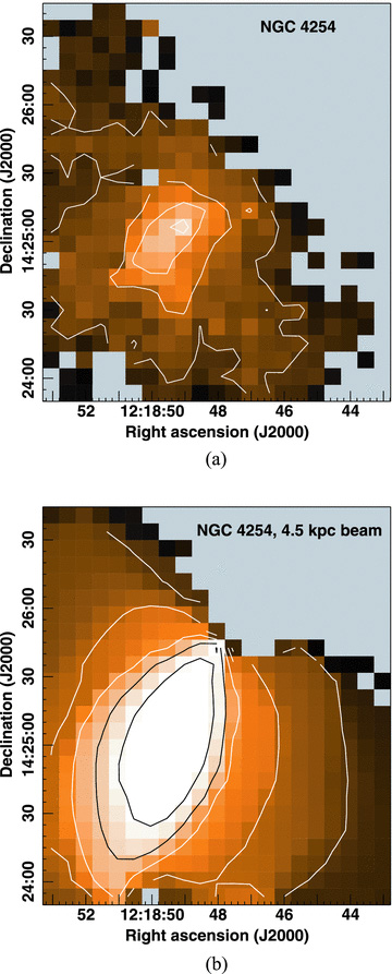
(a) CO J = 3–2 velocity dispersion for NGC 4254 at the native resolution of the JCMT data (14.5 arcsec or 1.15 kpc at a distance of 16.7 Mpc). Colour scale runs from 0 to 60 km s−1 and the contours are 10, 20, 30, 40 and 50 km s−1. (b) CO J = 3–2 velocity dispersion for NGC 4254 smoothed to a resolution of 4.5 kpc (56 arcsec) to match the resolution of observations of disc galaxies at z∼ 1 of Tacconi et al. (2010). Colour scale and contours are the same as in (a).
The average values of 20–30 km s−1 seen at low resolution in the discs of these three galaxies are quite similar to the value of ∼20 km s−1 found in EGS13035123 by Tacconi et al. (2010). EGS13035123 has 10–20 times the star formation rate, H2 gas mass and stellar mass compared to NGC 4254 (Kennicutt et al. 2003; Kranz et al. 2003; Wilson et al. 2009). However, EGS13035123 is also roughly a factor of 3 larger in its CO radius than NGC 4254 (Wilson et al. 2009), which implies that the gas surface density, stellar surface density and star formation rate surface density inside the molecular discs of these two galaxies are quite similar. Thus, the similar velocity dispersions between the two galaxies are likely related to the similar mass surface densities in the disc. The two galaxies also have quite similar molecular gas fractions of ∼0.25 (Kranz et al. 2003; Wilson et al. 2009; Tacconi et al. 2010). This comparison supports a picture where the high star formation rates seen at z = 1 may be at least partly due to the presence of physically larger molecular gas discs at this epoch.
5 CONCLUSIONS
We have used large-area high velocity resolution CO J = 3–2 observations of 12 nearby galaxies to study the vertical velocity dispersion in the dense molecular gas. Three of the galaxies show a roughly constant velocity dispersion as a function of radius, while the other nine galaxies have a central peak followed by a fall-off with radius to typically 0.2–0.4r25. Flat velocity dispersion profiles are seen only in some of the late-type spiral galaxies in our sample, and those with flat profiles have the lowest mass. The observed values of the velocity dispersion range from 4.1 to 20.1 km s−1. These velocity dispersions are comparable to the internal velocity dispersions of individual giant molecular clouds in our own and other galaxies (Solomon et al. 1987; Wilson & Scoville 1990). Correcting for these internal velocity dispersions yields an average cloud–cloud velocity dispersion of 6.1 ± 1.0 km s−1 measured over nine galaxies with good radial profiles. This cloud–cloud velocity dispersion is comparable to recent measurements in our own Galaxy (Stark & Lee 2005, 2006) and M33 (Wilson & Scoville 1990).
A direct comparison with the high-resolution H i maps from the THINGS survey (Walter et al. 2008) in six galaxies shows that the cloud–cloud velocity dispersion is on average twice as small as the velocity dispersion of the atomic gas, which implies a much smaller scaleheight for the molecular gas. Theoretical analyses of the stability of multicomponent discs suggest that the dynamically coldest component is the most important in driving instability (Jog & Solomon 1984a,b; Rafikov 2001). This analysis suggests that it is the properties of the dense molecular gas, rather than the atomic gas, that are the most important for determining whether galactic discs are stable against gravitational collapse, especially where the mass of the ISM is H2 dominated.
The cloud–cloud velocity dispersion is correlated at the 95 per cent confidence level with both the far-infrared luminosity and the K-band absolute magnitude. Thus, as for the atomic gas, we find evidence that star formation activity (as traced by the infrared luminosity) tends to increase the velocity dispersion in the dense molecular gas. The correlation with K magnitude, which traces the total stellar mass, implies that the cloud–cloud velocity dispersion is also enhanced in more massive galaxies.
We have used our data to examine the apparent kinematical properties of the molecular disc at a spatial resolution of 4.5 kpc chosen to match the best resolution for galaxies at redshifts of 1–2 (Tacconi et al. 2008). A degradation of the resolution from 1.2 to 4.5 kpc results in an increase in the average velocity dispersion in the outer disc by a factor of 2. The average velocity dispersion of NGC 4254 viewed with 4.5-kpc resolution is quite comparable to the velocity dispersion of 20 km s−1 seen in a normal galaxy at z = 1 (Tamburro et al. 2009). Both galaxies have comparable gas and stellar surface densities, as well as star formation rate surface densities, which suggests that the higher star formation rates seen at z = 1 may be partly attributed to the presence of physically larger molecular discs. This analysis suggests that this data set can provide a valuable local benchmark in understanding lower spatial resolution observations of galaxies in the early Universe.
cupid is part of the starlink (Currie et al. 2008) software package, which is available for download from http://starlink.jach.hawaii.edu.
We thank the anonymous referee for a referee report which spurred us to re-examine our data processing choices and resulted in a significant improvement in the paper. The James Clerk Maxwell Telescope is operated by The Joint Astronomy Centre on behalf of the Science and Technology Facilities Council of the United Kingdom, the Netherlands Organisation for Scientific Research and the National Research Council of Canada. The research of JI and CDW is supported by grants from NSERC (Canada). AU has been supported through a Post-Doctoral Research Assistantship from the UK Science & Technology Facilities Council. Travel support for BEW and TW was supplied by the National Research Council (Canada). We acknowledge the usage of the HyperLeda data base (http://leda.univ-lyon1.fr) and thank R.N. Henriksen for useful discussions. This research has made use of the NASA/IPAC Extragalactic Database (NED) which is operated by the Jet Propulsion Laboratory, California Institute of Technology, under contract with the National Aeronautics and Space Administration.
REFERENCES
Appendices
APPENDIX A: COMPARISON WITH PREVIOUS PROCESSING METHODS
There are two different methods that have been used to measure velocity dispersions in molecular gas in galaxies. Combes & Becquaert (1997) measured velocity dispersions in NGC 628 and 3938 by fitting Gaussian profiles to individual spectra, while Walsh et al. (2002) used moment 2 maps of NGC 6946 to determine the average velocity dispersion. While the moment 2 maps used in this paper are easier to compute and analyse than fitting individual profiles to many hundreds of spectra, they can potentially be subject to some systematic effects depending on choices made in the processing. We investigate some of these effects here by comparing our data and moment 2 maps for NGC 628 and 3938 with the results given by Combes & Becquaert (1997) for the same galaxies.
We first investigated whether the measured velocity dispersion was affected by the angular and spectral resolution of the data. The CO J = 1–0 data from Combes & Becquaert (1997) have an angular resolution of 23 arcsec and a spectral resolution of 2.6 km s−1, while the JCMT CO J = 3–2 data have an angular resolution of 14.5 arcsec and a spectral resolution of 0.43 km s−1. We produced three additional data cubes for each galaxy: one binned by six channels in velocity, one convolved to achieve a Gaussian beam of 23 arcsec and one that was both convolved and binned. From these cubes, we made moment 2 maps using the method described in Section 2 but using a signal-to-noise ratio cut-off for the mask of 3.5σ so as to include only regions with a relatively high signal-to-noise ratio. The average velocity dispersion measured in each map is given in Table A1. These results clearly show that data with poorer spectral or spatial resolution will give higher values for the velocity dispersion than data with better spectral or spatial resolution. The data also suggest that spatial resolution may be a more important factor in increasing the measured velocity dispersion than spectral resolution, as long as the spectral resolution is sufficient to resolve the lines. Interestingly, our average velocity dispersions for these two galaxies are only slightly smaller than those measured by Combes & Becquaert (1997) when our data are smoothed spatially and spectrally to match their data.
Velocity dispersions measured with different spectral and spatial resolutions.
| Data cube useda | NGC 3938 | NGC 628 |
| Original | 3.7 | 3.1 |
| Binned to 2.6 km s−1 | 4.8 | 3.9 |
| Convolved to 23-arcsec Gaussian | 6.5 | 4.2 |
| Convolved and binned | 7.4 | 4.7 |
| Combes & Becquaert (1997) | 9 | 6.5 |
| Data cube useda | NGC 3938 | NGC 628 |
| Original | 3.7 | 3.1 |
| Binned to 2.6 km s−1 | 4.8 | 3.9 |
| Convolved to 23-arcsec Gaussian | 6.5 | 4.2 |
| Convolved and binned | 7.4 | 4.7 |
| Combes & Becquaert (1997) | 9 | 6.5 |
a All values measured for the CO J = 3–2 line in km s−1.
Velocity dispersion measured using a signal-to-noise ratio cut-off of 3.5σ.
We next investigated the effect of the choice of the signal-to-noise ratio cut-off for the masks used in creating the moment map. For this analysis, we used the data cubes that had been smoothed spatially to match the data from Combes & Becquaert (1997) to give a better signal-to-noise ratio in our maps, but which had no spectral smoothing applied. The results are given in Table A2. It is clear that the measured velocity dispersion decreases systematically as higher signal-to-noise ratio cut-offs are used in the mask.
Velocity dispersions measured with different signal-to-noise ratio cut-offs for mask.
| Signal-to-noise ratio cut-off useda | NGC 3938 | NGC 628 |
| 5σ | 3.8 | 3.4 |
| 4.5σ | 4.8 | 3.7 |
| 4.0σ | 5.7 | 3.9 |
| 3.5σ | 6.5 | 4.2 |
| 3.0σ | 7.2 | 4.6 |
| 2.5σ | 9.1 | 5.3 |
| Combes & Becquaert (1997) | 9 | 6.5 |
| Signal-to-noise ratio cut-off useda | NGC 3938 | NGC 628 |
| 5σ | 3.8 | 3.4 |
| 4.5σ | 4.8 | 3.7 |
| 4.0σ | 5.7 | 3.9 |
| 3.5σ | 6.5 | 4.2 |
| 3.0σ | 7.2 | 4.6 |
| 2.5σ | 9.1 | 5.3 |
| Combes & Becquaert (1997) | 9 | 6.5 |
a All values measured for the CO J = 3–2 line in km s−1.
Finally, we performed Gaussian fits to selected spectra from the data cube of NGC 3938 that had been convolved to 23 arcsec and binned to 2.6 km s−1 resolution (Fig. A1 and Table A3). To mimic approximately the selection of spectra shown in Combes & Becquaert (1997), we selected the spectrum with the highest velocity dispersion in a map made with a 3.5σ cut-off and then stepped away from this spectrum in steps of 3 pixels (21.8 arcsec) in the north and south directions. We obtain similar values for the velocity dispersions from fits to the unbinned spectra; binned spectra are shown in Fig. A1 for clarity. Although there is considerable scatter in the velocity dispersions for individual spectra, the average value derived from Gaussian fits is 1.2 times larger (the standard deviation of 0.4) than the value derived from the moment 2 map.
Observed CO J = 3–2 emission at five positions in NGC 3938. The spectra have been convolved to a 23-arcsec beam and binned to 2.6 km s−1 resolution. Spectra are spaced by 22 arcsec along the declination axis ordered from north (top) to south (bottom) and the central spectrum corresponds to (11:52:49.6, 44:07:17.7). Gaussian fits to each spectrum are overlaid; the bar indicates the region used to obtain the fit.
Comparison of velocity dispersion from Gaussian fits and second moment maps for selected positions in NGC 3938.
| Positiona (arcsec, arcsec) | Gaussian fit (km s−1) | Moment 2 mapb (km s−1) |
| (0, 44) | 9.4 ± 2.9 | 7.8 |
| (0, 22) | 14.0 ± 2.3 | 19.3 |
| (0, 0) | 23.0 ± 4.4 | 19.3 |
| (0, −22) | 8.7 ± 1.3 | 8.4 |
| (0, −44) | 15.0 ± 3.2 | 8.2 |
| Positiona (arcsec, arcsec) | Gaussian fit (km s−1) | Moment 2 mapb (km s−1) |
| (0, 44) | 9.4 ± 2.9 | 7.8 |
| (0, 22) | 14.0 ± 2.3 | 19.3 |
| (0, 0) | 23.0 ± 4.4 | 19.3 |
| (0, −22) | 8.7 ± 1.3 | 8.4 |
| (0, −44) | 15.0 ± 3.2 | 8.2 |
a All values measured for the CO J = 3–2 line. The spectra have been convolved to a 23-arcsec beam and binned to 2.6 km s−1 resolution. (0, 0) corresponds to (11:52:49.6, 44:07:17.7 J2000).
b Measured from maps made using a 2.5σ cut-off.
On the basis of this analysis, we opted to use a signal-to-noise ratio cut-off of 2.5σ on our original data cubes, as this choice seemed to give good agreement with the results from Combes & Becquaert (1997) when both data sets were matched in angular and frequency resolution.
APPENDIX B: THE POSSIBLE EFFECT OF ANISOTROPIES IN THE VELOCITY DISPERSION
There is no statistically significant correlation of velocity dispersion in the molecular gas with inclination in our data (Fig. B1). The average observed velocity dispersion is 5.3 km s−1 for the four galaxies with inclinations of <25° and 8.1 km s−1 for the eight galaxies with inclinations of >25°, and these values agree within 2σ. We have also checked for any correlation of the velocity dispersion normalized by each of the star formation rate and D25 with inclination and again found no correlation.
For an inclined galaxy, the observed velocity dispersion is a combination of the in-plane (σr, σθ) and vertical velocity (σz) dispersions. We will assume that σr=σθ and will refer to the in-plane component of the velocity dispersion as σr from here on for simplicity. Thus, for a galaxy with inclination i, the observed velocity dispersion is  . If the radial and vertical velocity dispersions of the molecular gas were isotropic, we would not expect any trend of velocity dispersion with inclination. If, however, the velocity ellipsoid of the giant molecular clouds (which contain most of the mass of the molecular ISM) is anisotropic, with σr > σz, then the observed velocity dispersion would tend to increase with increasing inclination.
Unfortunately, there is no direct information on the shape of the velocity ellipsoid for giant molecular clouds. In theoretical models, the cloud velocity dispersion has been attributed to cloud–cloud scattering (Gammie et al. 1991) as well as to the driving effects of spiral structure (Thomasson et al. 1991). Since both these models were two dimensional, they can give us no guidance on the relative strength of the vertical and in-plane velocity dispersions.
In contrast, there have been a number of studies of the stellar velocity ellipsoid (Delhaye 1965; Dehnen & Binney 1998; Elias, Alfaro & Cabrera-Caño 2006). If the velocity ellipsoid of any stars can give us a clue to that of GMCs, it will be the youngest O- and B-type stars, which may be sufficiently young to still trace the motions of their parent clouds. The largest values for the velocity ellipsoid can be found in Delhaye (1965), who measured a relative velocity dispersion σz/σr = 0.75 for 35 O–B5 supergiants. Dehnen & Binney (1998) measure a significantly smaller value of σz/σr = 0.38+0.5−0.10 for 500 main-sequence stars with −0.24 < B−V < 0.14. However, this colour range extends well into the A star range where main-sequence lifetimes are larger than 100 Myr. Since this velocity dispersion ratio is well known to decrease with the age of the stellar population (Delhaye 1965; Dehnen & Binney 1998), this value may not be an appropriate one to adopt for GMCs. In a recent study of OB stars using Hipparcos data, Elias et al. (2006) obtained a value of σz/σr = 0.64 ± 0.06 for 800 stars with spectral types O–B6 within 1 kpc of the Sun. Dividing the sample into stars in Gould’s Belt and the Local Galactic Disc results in values of σz/σr = 0.72 ± 0.08 and σz/σr = 0.57 ± 0.09, respectively.
Gammie et al. (1991) caution that a critical difference between star–cloud and cloud–cloud scattering, namely the relative sizes of the epicyclic amplitude and the cloud tidal radius, prevents direct application of stellar results to molecular clouds. However, this model ignores the possible effect of spiral arms, which could conceivably introduce an anisotropy into the cloud motions. In estimating the possible correction to our observed velocity dispersions for the effects of anisotropy in the velocity ellipsoid, we adopt a conservative value of σz/σr = 0.6, which is the 1σ upper limit obtained by Elias et al. (2006) for their entire sample. With this value, corrections for the velocity ellipsoid only exceed 10 per cent for inclinations greater than 27°.
