


Abstract
Among the 48 known multiplanetary systems, some are in mean-motion resonances (in most cases in the 2:1 mean-motion resonance). Although until now no extrasolar planetary systems have been found in a 1:1 mean-motion resonance, many studies are dealing with this configuration. Besides the well-known motion of the Trojan asteroids, further possibilities exist for stable configurations of planets or satellites in a 1:1 resonance. For one thing, we can find so-called exchange orbits in our Solar system (Janus and Epimetheus), where both Saturnian moons exchange the values of their semi-major axes (exchange-a configuration) when approaching each other. In addition, we can also find similar behaviour for two planets on orbits with the same semi-major axis, but with different eccentricities; here an exchange of eccentricities takes place (exchange-e configuration). In this work we focused on the second possibility and performed a parameter study by varying the initial conditions (mass and eccentricity) of two planets on exchange-e orbits. By means of an extensive numerical study, we can find a wide variety of initial conditions leading to long-term stable orbits.
1 INTRODUCTION
At present (2010) we know of more than 450 extrasolar planetary systems, of which 48 are multiplanetary systems (shown in the Extrasolar Planets Encyclopedia maintained by J. Schneider1). Some of them move in mean-motion resonances (MMRs). Until now, most resonant multiplanetary systems found have been in a 2:1 MMR (e.g. Voyatzis, Kotoulas & Hadjidemetriou 2009), but, by analysing radial velocity curves, theoretical studies (e.g. Goździewski, Mikaszewski & Musieliński 2008) have shown that the signals of 2:1 MMRs of circular orbits are ambiguous and may also be modelled by a 1:1 MMR. Many general studies deal with the possibilities for forming resonant extrasolar planetary systems or for planets being captured in resonances during the migration process, e.g. Thommes (2005), Beaugé et al. (2007), Raymond et al. (2008) and Cresswell & Nelson (2009).
In this study, we treat the problem of long-term stable motion of two celestial bodies in a 1:1 MMR. Different co-orbital configurations are known, where the most common one is the Trojan configuration. A variety of studies have been published about the possibility of terrestrial planets orbiting in the Lagrangian points of known extrasolar planets (see e.g. Laughlin & Chambers 2002; Nauenberg 2002; Dvorak et al. 2004; Érdi & Sándor 2005; Schwarz et al. 2007, 2009) and studies on the capture of Trojans during planetary migration (see e.g. Morbidelli et al. 2005; Lykawka & Horner 2010) have also been carried out.
Besides the Trojan orbits in their two forms, namely libration around one of the Lagrangian points (the tadpole orbits) and motion around both Lagrangian points (the horseshoe orbits), we can distinguish two types of so-called exchange orbits.
Exchange-a configuration. Two celestial bodies (planets or satellites) are moving on nearly circular orbits with almost the same semi-major axis around a much more massive host star. Because of the third Keplerian law, the one with the inner orbit is faster and approaches the outer one. Before they meet, the inner planet is shifted to the orbit of the outer and the outer planet moves inward (orbit with a smaller semi-major axis); this means that they have changed their orbits (see Fig. 1). Bodies in exchange-a orbits periodically exchange their semi-major axes a (e.g. Spirig & Waldvogel 1985; Auner 2001; Dvorak 2006), which can be seen as a generalization of the aforementioned horseshoe orbits for the non-restricted three-body problem. They can also be found in our Solar system; the two moons of Saturn Janus and Epimetheus show such a motion.
Exchange-e configuration. Two planets are moving on orbits with the same semi-major axis around a much more massive central body, the first one on a circular and the second one on an eccentric orbit. They ‘exchange’ their eccentricity (two examples are shown in Fig. 2) because the initial circular orbit transfers angular momentum to the planet on the eccentric orbit and vice versa. Planets in exchange-e orbits periodically exchange the value of their eccentricities.
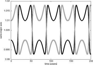
Exchange-a configuration: in this example both planets have a mass of 10−5 M⊙ and move on circular orbits in the same plane. The mean anomaly of planet 1 is 0° and that of planet 2 is 180°. The semi-major axis of planet 1 (black line) initially equals 1 au, while the semi-major axis of planet 2 (grey line) is initially 1.001 au.
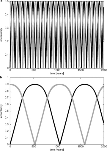
Eccentricity of the two planets versus time. In both cases the mass ratio was set to μ = 0.001. For the upper graph the initial eccentricity of planet 2 was e = 0.5 and for the lower graph e = 0.9. All other initial conditions were as described in Table 1.
In particular, the study by Laughlin & Chambers (2002) gives information about the underlying analytics. Numerical studies were carried out by Roth (2009) and Nauenberg (2002). Nauenberg (2002) discussed the possibilities for detecting such exchange-e orbits in extrasolar planetary systems. He showed that, with the aid of radial velocity measurements, such orbits could be distinguishable from the case of a single planet and they are long-term stable.
In the present work, we focus on the exchange-e configuration and determine the dependence of stable regions on the mean anomaly and the eccentricity of the planets. In Section 2 we introduce the model and methods used, in Section 3 we present the results of our investigation for the low-mass region and in Section 4 for the high-mass region. In Section 5 we determine the percentage of stable orbits in both regions and in Section 6 check the periods for exchange of eccentricities. In the last section our conclusions are drawn and possible extensions of this study are briefly discussed.
2 THE DYNAMICAL MODEL AND THE METHODS
We performed integrations for 106 yr in the planar three-body problem, consisting of a host star of 1 M⊙ and two massive planets with the same mass. All calculations were made by direct numerical integration with the Lie integration method (see Hanslmeier & Dvorak 1984; Lichtenegger 1984; Delva 1984, 1985; Dvorak & Freistetter 2005; Eggl & Dvorak 2010), which is capable of dealing with high eccentric orbits and close encounters between bodies.
A schematic plot for the initial conditions in the exchange-e configuration that we used for our investigation is shown in Fig. 3. As described there, one planet initially had a circular orbit, while the other one was started on an eccentric orbit. We divided the study into two main parts according to the mass ratio μ:2
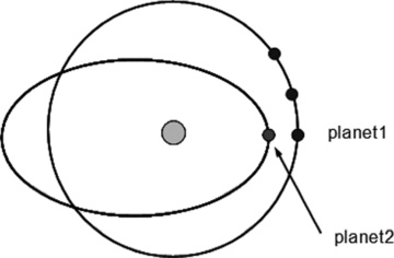
Schematic plot for the initial exchange-e configuration: planet 1 was always started on a circular orbit with different mean anomalies, while planet 2 was initially placed on different eccentric orbits with a zero mean anomaly.
the low-mass region μ≤ 0.001 and
the high-mass region, for mass ratios of planets 0.001 ≤μ≤ 0.02; from this μ onward, no stable orbits in the exchange-e configuration were found.
In Table 1 we show in detail the initial conditions for both studies; for the low-mass region 13 different values for the masses of the planets were taken, which can be seen in Table 2. For the high-mass region the masses of the planets were equally distributed with Δμ = 0.001; we used a finer grid for the eccentricities for these systems (see Table 1, lower part).
Initial conditions for the two planets in the exchange-e configuration. Upper part: low-mass region; lower part: high-mass region. The mass of the star was always 1 M⊙ and the semi-major axes of the planets were set to 1 au.
| Planet 1 | Planet 2 | |
| e | 0.0 | 0.1–0.9, Δe = 0.1 |
| M[deg] | 0–180, ΔM = 1 | 0 |
| Mass [M⊙] | 10−6≤m≤ 0.001 | |
| e | 0.0 | 0.05–0.9, Δe = 0.05 |
| M[deg] | 0–180, ΔM = 2 | 0 |
| Mass [M⊙] | 0.001 ≤m≤ 0.02 | |
| Planet 1 | Planet 2 | |
| e | 0.0 | 0.1–0.9, Δe = 0.1 |
| M[deg] | 0–180, ΔM = 1 | 0 |
| Mass [M⊙] | 10−6≤m≤ 0.001 | |
| e | 0.0 | 0.05–0.9, Δe = 0.05 |
| M[deg] | 0–180, ΔM = 2 | 0 |
| Mass [M⊙] | 0.001 ≤m≤ 0.02 | |
Parameters a, b, c and d for different masses of the two planets in exchange orbits. The numbers ‘1’, ‘2’ and ‘3’ correspond to the lines shown in Fig. 4.
| Mass | Border | a | b | c | d |
| 10−6 | 1 | −305.56 | 378.57 | −188.37 | 201.21 |
| 2 | 106.06 | −84.85 | 134.74 | 0.07 | |
| 3 | −105.22 | 167.57 | 40.43 | 5.06 | |
| 2 × 10⁻⁶ | 1 | −250.00 | 283.33 | −136.55 | 192.36 |
| 2 | 146.46 | −129.87 | 151.26 | −1.43 | |
| 3 | −120.37 | 186.29 | 31.02 | 6.13 | |
| 5 × 10⁻⁶ | 1 | −191.92 | 191.23 | −91.58 | 185.79 |
| 2 | 267.68 | −250.65 | 185.59 | −2.71 | |
| 3 | −63.13 | 94.16 | 66.48 | 2.93 | |
| 7 × 10⁻⁶ | 1 | −90.91 | 38.20 | −20.27 | 175.36 |
| 2 | 224.75 | −196.86 | 166.88 | −0.43 | |
| 3 | −51.35 | 68.90 | 80.50 | 0.82 | |
| 10−5 | 1 | −101.01 | 104.22 | −78.57 | 185.64 |
| 2 | 227.27 | −204.44 | 170.38 | 0.14 | |
| 3 | −53.87 | 65.55 | 84.71 | −0.33 | |
| 2 × 10⁻⁵ | 1 | 126.26 | −106.17 | −52.36 | 185.43 |
| 2 | 242.42 | −229.65 | 179.13 | 1.43 | |
| 3 | −66.50 | 64.14 | 92.08 | −1.94 | |
| 5 × 10⁻⁵ | 1 | −434.34 | 860.17 | −514.4 | 222.00 |
| 2 | 255.05 | −263.96 | 198.20 | 1.93 | |
| 3 | −69.02 | 24.10 | 130.48 | −11.56 | |
| 7 × 10⁻⁵ | 1 | −573.23 | 1062.60 | −584.68 | 218.14 |
| 2 | 242.42 | −258.23 | 200.56 | 2.57 | |
| 3 | −53.03 | −4.33 | 141.53 | −13.57 | |
| 10−4 | 1 | −313.13 | 629.87 | −344.12 | 169.21 |
| 2 | 148.99 | −114.83 | 131.31 | 13.93 | |
| 3 | −114.48 | 82.22 | 105.32 | −10.49 | |
| 2 × 10⁻⁴ | 1 | 35.35 | 118.94 | −102.75 | 124.43 |
| 2 | 138.89 | −120.24 | 140.40 | 15.86 | |
| 3 | −190.24 | 200.51 | 46.95 | −5.61 | |
| 5 × 10⁻⁴ | 1 | −217.17 | 463.42 | −200.30 | 120.14 |
| 2 | 113.64 | −99.24 | 136.56 | 21.07 | |
| 3 | −357.74 | 440.84 | −56.15 | 0.30 | |
| 7 × 10⁻⁴ | 1 | −73.23 | 228.03 | −94.32 | 97.79 |
| 2 | 123.74 | −112.88 | 137.24 | 24.36 | |
| 3 | −334.18 | 427.45 | −69.39 | 2.08 | |
| 0.001 | 1 | −75.76 | 279.65 | −144.13 | 105.57 |
| 2 | 32.83 | −5.63 | 104.35 | 29.29 | |
| 3 | −472.22 | 640.48 | −174.48 | 16.69 |
For the distinction between stable and unstable motion, two criteria were used that provided the same results: (1) a direct investigation of the eccentricity with respect to change of its exchange period (see Fig. 2) was one criterion (used mainly for the low-mass region). To be regarded as stable, an orbit has to fulfil the following two criteria: after each exchange period (Pe± 0.5 per cent) the initially circular orbit has to be returned to its initial state (ePlanet1 = 0.0 ± 0.5 per cent). (2) As another tool, we used the deviation Δa from the initial semi-major axes (used mainly for the high-mass region). It turned out that Δa < 0.021 was a good stability criterion, but both methods were used in complementary fashion.
3 THE LOW-MASS REGION

Initial condition diagrams, where the eccentricity of planet 2 versus the mean anomaly of planet 1 is plotted. The two planets have mass ratios of (a) μ = 7 × 10⁻⁵ and (b) μ = 0.001. The unstable region (grey region) increases with mass ratio; the black lines on the border between the stable (white background) and unstable (grey background) regions are the respective least-squares fits (labelled 1, 2 and 3; see equation 1).
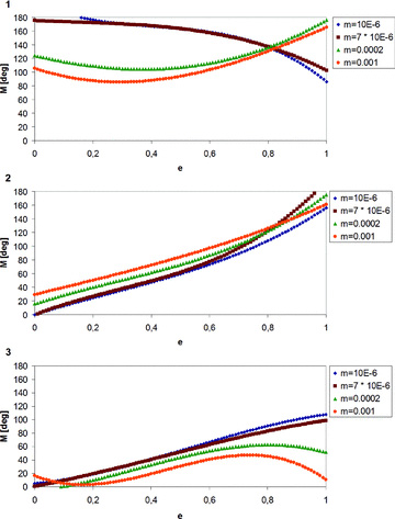
Least-squares fits for four selected mass ratios: μ = 10−6, 7 × 10⁻⁶, 2 × 10⁻⁴ and 0.001. Upper panel: lower border of the upper unstable region, labelled with ‘1’ in Fig. 4. Middle panel: upper border of the lower unstable region, labelled with ‘2’ in Fig. 4. Lower panel: lower border of the lower unstable region, labelled with ‘3’ in Fig. 4.
The least-squares fits of border ‘1’ have a different shape for small and large mass ratios: for small values of μ the curves have a concave shape and they gradually decrease with larger eccentricities; for larger values they have a minimum value around e = 0.3 and they have a convex shape. It is interesting to note that the curves have a common point for e∼ 0.8 and M∼ 140°. Line ‘2’ does not show a significant dependence on the mass ratio, and the curve is slightly increasing with the eccentricities and the difference in mean anomaly; the shape is convex. For line ‘3’ (again see Fig. 5 for the low mass ratios, up to ≈2 × 10⁻⁶) the curves do not change much and they are almost linear. One can see a modification for larger mass ratios: from a value of ≈5 × 10⁻⁵ onward the least-squares fits remain quite similar, again with a concave shape, and reach a maximum value around e∼ 0.8 and M∼ 50°.
4 THE HIGH-MASS REGION
As mentioned, for the mass ratios 0.001 ≤μ≤ 0.02 we used a constant Δμ = 0.001, a finer grid for the eccentricities (Δe = 0.05) and the stability criterion 2 (Δa). To compare the results of both stability criteria, we started to determine a plot for a lower mass ratio (μ = 7 × 10⁻⁵) for which we show the escape time according to criterion 2 in Fig. 6. There the grey-scale corresponds to the escape time (black = short escape times, light grey = stable configuration for the whole integration time), which we defined as the time at which Δa reaches a value higher than 0.021 au. It is clearly visible that the border between stable and unstable motion is again quite sharp. In fact the orbits of the two planets very soon turned out to be unstable, or they stayed in a stable configuration for the whole integration time. For the low-mass region we used stability criterion 1 (the eccentricity), for the high-mass region stability criterion 2 (Δa). The agreement between these two methods is excellent, which one can see by comparing Figs 4 and 6. Additionally, we show the results of the corresponding least-squares fits (black circles in Fig. 6) in order to compare the Δa results with our first results.
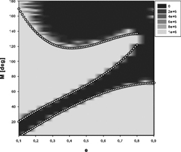
Initial condition diagrams, where the eccentricity of planet 2 versus the mean anomaly of planet 1 is plotted. The two planets have mass ratios of μ = 7 × 10⁻⁵. The unstable black regions correspond to the unstable grey regions of Fig. 4, while the grey-scale corresponds to the escape time (defined as the time at which Δa reaches a value higher than a = 0.021 au). The black circles mark the least-squares fits of the border and are defined in Table 2.
For higher mass ratios, the determination of a least-squares fit is useless, since the stable regions shrink to a few stable orbits on the M versus e plots. To visualize this we show in Fig. 7 the results for three different mass ratios (μ = 0.001, 0.002 and 0.003). As one can see already for a μ of 0.005, not many stable orbits are left. Nevertheless we could find some stable orbits up to a mass ratio of 0.019. For μ > 0.013 just a few (fewer than 10) stable orbits could be found, which – as long-term integrations showed – remain in a stable configuration up to an integration time of 107 yr.
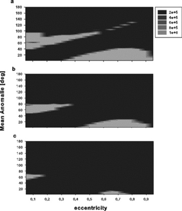
The plots show the eccentricity of planet 2 versus the mean anomaly of planet 1, where the planets have three different mass ratios: μ = 0.001 (upper), 0.002 (middle) and 0.005 (lower). The grey-scale corresponds to the escape time (defined as the time at which Δ a reaches a value higher than 0.021 au).
5 SHRINKING OF THE STABLE REGIONS WITH MASS RATIO μ
In a further step we determined the fractional area of the stable region for each mass ratio μ. In Fig. 8 (upper graph) we plot the percentage of stable orbits versus the mass ratio (logarithmic scale) for the low-mass region. One can see that the stable region rapidly shrinks. For the high-mass region (note that now the y-axis, denoting the percentage of stable orbits, is on a logarithmic scale) there is a smooth decrease of the stable region up to a mass ratio of μ = 0.015, for which we could find no stable orbits. For μ≥ 0.017 again a few stable orbits can be found, until the final stability limit is reached for μ = 0.019. The results agree quite well with the theory (see Marchal 1990, p. 48; also Laughlin & Chambers 2002), predicting an unstable region around ε = 2mPlanet/(2mPlanet+mStar) = 0.030 and a final stability limit at 0.03812 in the three-body problem. Note that the different values for the stability limit occur because of different definitions of the mass ratio: while we use μ=mPlanet/(mPlanet+mStar), Marchal (1990) and Laughlin & Chambers (2002) use ε = 2mPlanet/(2mPlanet+mStar).
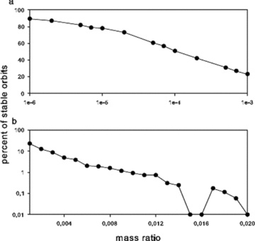
On the x-axis we plot the mass ratio and on the y-axis the percentage of stable orbits. (a) Results for the low-mass region (10−6≤μ≤ 0.001); (b) results for the high-mass region (0.001 ≤μ≤ 0.020).
6 THE EXCHANGE PERIODS
We also investigated how the exchange period4Pe depends on the mass, eccentricity and mean anomaly of the two planets. In Fig. 2 we show the eccentricity of both planets versus time for μ = 0.001 and two different initial eccentricities ((a) e = 0.5 and (b) e = 0.9). Here it is clearly visible that Pe increases significantly with larger eccentricities for the same mass ratio μ.
For a more systematic study, we calculated Pe for all integrated orbits; in Fig. 9 we show as examples the respective results for three eccentricities e = 0.1, 0.5 and 0.9 and four different mass ratios (μ = 10−6, 7 × 10⁻⁶, 0.0002 and 0.001). Note that for the orbits with Pe larger than 106 the integrations were extended for an appropriately longer time. In these figures we plotted the initial mean anomalies (M = 0°–180° with ΔM = 10°) versus Pe in years. As one can see, the shape of the curve depends primarily on the eccentricity.
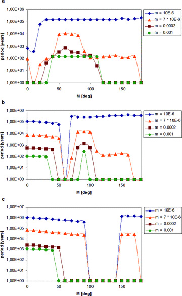
On the x-axis we plot the mean anomaly and on the y-axis Pe in years. The four different symbols correspond to different mass ratios (see legend). The three plots show the results for three initial eccentricities of planet 2: (a) e = 0.1, (b) e = 0.5 and (c) e = 0.9.
For e = 0.1 (Fig. 9a), ‘Pe’ has a window of unstable orbits close to M = 0°, which is understandable because the starting positions (compare with Fig. 3) of the two planets are quite close to each other. In addition, for larger initial values of M another unstable window occurs that extends up to M = 180° only for μ = 0.001 and μ = 0.0002. The difference in Pe is very large for the different masses (102 < Pe < 105 yr).
For e = 0.5 (Fig. 9b), the unstable window is shifted to M∼ 50° and becomes broader with larger masses. Also interesting to note is the length of the periods compared with e = 0.1 (Fig. 9a): globally they have almost the same value.
For e = 0.9 (Fig. 9c), all periods are an order of magnitude larger compared with e = 0.1 and e = 0.5. The unstable window is again shifted towards larger values of M∼ 110° and increases significantly with large masses μ.
In conclusion, for the periods one can say that with larger masses the periods Pe decrease; in contrast, with larger eccentricities they increase. Pe does not seem to depend much on the initial mean anomaly, with the exception that for some values there exists an instability window.
7 CONCLUSIONS
The goal of the present work was to determine the dependence of stable regions on the masses involved, the mean anomaly and the eccentricities of the planets in exchange-e configuration. We were able to define least-squares fits for the borders of the stable region for each mass ratio of the lower-mass region. Additionally we showed that the stable region shrinks with larger μ and disappears completely for μ > 0.019.
We furthermore analysed the period of the exchange in eccentricity and showed that it depends on the masses of the planets and on their initial eccentricity. For rising mass ratios, we found decreasing periods (by the same factor as the mass ratio), while higher eccentricities always led to longer periods.
All in all, we can conclude that a wide variety of stable configurations exist in the 1:1 MMR besides Trojan motion and the exchange-a configuration. We found that exchange-e configurations remain stable to eccentricities as high as e = 0.9. An extension to different mass ratios of the two planets, slightly different semi-major axes and inclined orbits is in preparation. For these more realistic situations, it should even be possible to observe interesting planet pairs in extrasolar planetary systems with the aid of radial velocity measurements and, in rare cases, in transit observations.
μ=mPlanet/(mPlanet+mStar).
This time was 106 yr and corresponds to the same number of periods in the stable region.
The time after planet 1 again reaches an eccentricity of e = 0.0.
BF acknowledges support by the Austrian FWF Erwin Schrödinger grant No. J2892-N16. RS acknowledges support by the MOEL grant No. 309. We thank S. Eggl for helpful suggestions that improved the paper.
REFERENCES
