Are brightest halo galaxies central galaxies?

Abstract

1 INTRODUCTION

According to the current paradigm of galaxy formation, all galaxies form as a result of gas cooling at the centre of the potential well of dark matter haloes. Structures form hierarchically, such that smaller haloes merge to form larger and more massive haloes. When a halo and its ‘central’ galaxy are accreted by a larger halo, it becomes a subhalo and its galaxy becomes a ‘satellite’ galaxy. In this paradigm, it is assumed that ram-pressure and tidal forces strip satellite galaxies of their gas reservoir, causing their star formation to be quenched shortly after having been accreted. The central galaxy (i.e. the galaxy with the lowest specific potential energy), however, continues to accrete new gas, and is also expected to cannibalize some of its satellites. Consequently, it is generally assumed that the central galaxy is the most luminous, most massive galaxy in a dark matter host halo, and that it resides at rest at the centre of the halo’s potential well. Following van den Bosch et al. (2005, hereafter vdB05), we will refer to this as the ‘central galaxy paradigm’ (CGP).

There are numerous areas of astronomy in which the validity of the CGP is an essential assumption, although this is rarely enunciated. Examples are various techniques to measure halo masses, such as satellite kinematics (e.g. McKay et al. 2002; van den Bosch et al. 2004; More et al. 2009), weak lensing (e.g. Mandelbaum et al. 2006; Johnston et al. 2007; Cacciato et al. 2009, hereafter C09; Sheldon et al. 2009b) and strong lensing (e.g. Kochanek 1995; Cohn et al. 2001; Koopmans & Treu 2003; Rusin et al. 2003). In addition, the CGP also features in halo occupation modelling, where assumptions have to be made regarding the distribution of galaxies within dark matter haloes in order to compute the galaxy–galaxy correlation function on small scales (e.g. Scoccimarro et al. 2001; Sheth et al. 2001; Yang, Mo & van den Bosch 2003; Zehavi et al. 2005; Zheng et al. 2005; Cooray 2005; van den Bosch et al. 2007; Tinker et al. 2008), and in algorithms developed to identify galaxy groups and clusters in photometric or spectroscopic redshift surveys (e.g. Yang et al. 2005a, 2007, hereafter Y07; Berlind et al. 2006; Koester et al. 2007).

Whether central galaxies actually comprise a special population has been debated for many years. However, recent analyses of galaxies in groups and clusters (e.g. Weinmann et al. 2006; Skibba, Sheth & Martino 2007; von der Linden et al. 2007; van den Bosch et al. 2008; Pasquali et al. 2009, 2010; Skibba 2009; Hansen et al. 2009) and halo model analyses of galaxy clustering (e.g. Skibba et al. 2006; Cooray 2006; van den Bosch et al. 2007; Skibba & Sheth 2009) have explicitly shown that central galaxies are indeed a distinct population and exhibit different properties (e.g. colour, star formation activity, AGN activity, morphology, stellar population properties) than satellite galaxies of the same stellar mass, and with different dependencies on the mass of their host halo. In addition, these studies have shown that central galaxy properties are strongly correlated with halo mass, while those of satellite galaxies only reveal a very weak dependence on the mass of the halo in which they orbit. However, it is important to realize that in virtually all of these studies, central galaxies are assumed to be the brightest (or most massive) halo galaxies. If this aspect of the CGP is not correct for a non-negligible fraction of all haloes, the differences between centrals and satellites found by these studies will have to be considered lower limits.

The validity of the CGP has been investigated by a number of authors. In particular, several recent, observational studies have shown that although most brightest halo galaxies (BHGs) are nearly at rest near the centroid of their group or cluster, or at the peak of the cluster X-ray emission, some of them are not (e.g. Beers & Geller 1983; Malumuth et al. 1992; Bird 1994; Postman & Lauer 1995; Zabludoff & Mulchaey 1998; Oegerle & Hill 2001; Yoshikawa, Jing & Börner 2003; Lin & Mohr 2004; von der Linden et al. 2007; Bildfell et al. 2008; Hwang & Lee 2008; Sanderson, Edge & Smith 2009; Coziol et al. 2009). These studies have focused on either cD galaxies in clusters or brightest cluster galaxies (BCGs) in general. It has been argued that most cD galaxies form a subpopulation of BCGs (e.g. Bernstein & Bhavsar 2001; Coziol et al. 2009) and may have grown by ‘cannibalizing’ smaller neighbouring galaxies.

In an early study, Beers & Geller (1983) analysed the spatial distribution of bright galaxies in 56 rich clusters and argue that cD galaxies tend to lie at local density peaks but not necessarily at the bottom of the potential well of the whole cluster. Oegerle & Hill (2001) found that, out of their sample of 25 Abell clusters, the cD galaxies of four of them have significant peculiar velocities relative to the cluster velocity. More recent studies have analysed the positions and velocities of BCGs. For example, in a study of 833 Sloan Digital Sky Survey (SDSS) clusters, von der Linden et al. (2007) found that 21 BCGs in their sample lie farther than 1 Mpc away from the mean galaxy in the cluster. Hwang & Lee (2008) found that the BCGs of two clusters out of a sample of 24 have significantly offset velocities and positions; these two clusters also appear to be in dynamical equilibrium. Recently, Coziol et al. (2009), using a sample of 452 Abell clusters selected for the likely presence of a dominant galaxy, estimated that the BCGs have a median peculiar velocity of 32 per cent of their host clusters’ radial velocity dispersion.

We emphasize that these results, based on large clusters, do not necessarily hold for less massive haloes. After all, in galaxy clusters, the ratio L₂/L₁ of the luminosities of the two brightest galaxies tends to be much smaller in a Milky Way (MW)-sized halo, on average (e.g. van den Bosch et al. 2007). For example, for the halo hosting the MW it is the ratio of the luminosities of the Large Magellanic Cloud and the MW, which is ∼0.1 (van den Bergh 1999), while this ratio is much closer to unity in Virgo, Coma and other nearby clusters (Postman & Lauer 1995). Consequently, it is only natural to expect that the CGP is more likely to be valid for low-mass haloes than for massive cluster-sized haloes. Nevertheless, vdB05 used a large sample of 3473 galaxy groups from the group catalogue of Yang et al. (2005a), and conclusively falsified the assumption that the brightest group galaxy is always at rest at the centre of the potential well. In this paper we extend the analysis of vdB05 using a larger, more accurate group catalogue, and focusing on different aspects of the CGP as a function of halo mass. In particular, we separately test two aspects of the CGP, namely (i) central galaxies reside at rest at the centre of their host halo’s potential well, and (ii) central galaxies are the brightest, most massive galaxies in their host haloes. We do so by comparing three hypotheses.

• ⁠: our null hypothesis is that the CGP is correct: central galaxies are always the brightest objects in their haloes and are at rest at the centre of the potential well.

• ⁠: central galaxies are the brightest objects in their haloes, but they have a velocity and spatial offset with respect to the centre of the potential well, such that the systems still obey the Jeans equations (i.e. they are still in dynamical equilibrium). We will specify the amount of offset via a velocity bias parameter, b_vel, to be defined in Section 4.2.

• ⁠: central galaxies reside at rest at the centre of the potential well, but they are not the brightest objects in a fraction f_BNC (for ‘brightest-not-central’) of all dark matter haloes.

In order to avoid confusion, throughout this paper we use the term ‘central galaxy’ to refer to the galaxy with the lowest specific potential energy. The central galaxy is the BHG in and ⁠, but not in ⁠, and its location coincides with the centre of the halo’s potential well in and ⁠, but not in ⁠.

We base our study on the galaxy group catalogue of Y07, extracted from the SDSS (York et al. 2000) Data Release 4 (DR4; Adelman-McCarthy et al. 2006). We analyse both the positions and velocities of BHGs relative to those of the other member galaxies, and compare the results to mock group catalogues that correspond to one of our three hypotheses. The large SDSS group catalogue, with accurate halo mass estimates, allows us to falsify and to quantify the degree to which and are valid (i.e. to constrain the values of b_vel and f_BNC).

This paper is organized as follows. In Section 2, we present two statistics that quantify the offsets of BHGs, and which can be used to assess deviations from the CGP. We describe the SDSS group catalogue in Section 3 and the construction of mock group catalogues in Section 4. In Section 5, we compare these mock catalogues to the data in order to test our three hypotheses. We find that both and can be ruled out, but that yields results in agreement with the data as long as 0.25 ≲f_BNC≲ 0.4, with a weak dependence on halo mass. In Section 6, we discuss our results and compare them to predictions from halo occupation statistics and from two semi-analytic models of galaxy formation. We also discuss the implications for studies of satellite kinematics. Finally, we end the paper with our conclusions and a discussion of additional implications of our results.

Throughout this paper, we adopt a flat Λcold dark matter (ΛCDM) cosmology with Ω_m = 0.238, Ω_Λ = 1 −Ω_m, n = 0.951, σ₈ = 0.744, and we express units that depend on the Hubble constant in terms of h≡H₀/100 km s⁻¹ Mpc⁻¹. In addition, we use ‘log’ as shorthand for the 10-based logarithm.

2 PHASE-SPACE STATISTICS OF CENTRAL GALAXIES

In order to test the CGP (i.e. hypothesis ⁠), we use the line-of-sight velocities of galaxies obtained from their redshifts. In what follows, v_BHG refers to the line-of-sight velocity of the BHG, and v_{sat, i} refers to the line-of-sight velocity of the ith satellite galaxy. We define the difference between the mean velocity of the satellite galaxies and that of the BHG. If the CGP is correct and v_{sat, i} follows a Gaussian distribution with velocity dispersion σ_sat, then the probability that a halo with N_sat satellite galaxies has a value of ΔV is given by

1

where ⁠. Therefore, in principle, one could define the parameter

2

and test the CGP by checking whether R follows a normal distribution with zero mean and unit variance. However, the velocity dispersion σ_sat is generally unknown, and instead we must use its unbiased estimator

3

Following vdB05, we use the following modified parameter as an indicator of the offset between BHGs and satellite galaxies:

4

This parameter is similar to the relative peculiar velocities of BCGs, |v_pec|/σ_cluster, used in the related studies (e.g. Malumuth et al. 1992; Coziol et al. 2009). If the null hypothesis of the CGP is correct, should follow a Student’s t-distribution with ν=N_sat− 1 degrees of freedom. Note that approaches a normal distribution with zero mean and unit variance in the limit N_sat→∞.

In practice, although the galaxy group finder (Yang et al. 2005a; Y07) has been thoroughly tested with mock SDSS catalogues to reliably identify galaxies residing in the same dark matter halo, it is not perfect. In particular, because of redshift errors and redshift-space distortions, the group finder inevitably selects some interlopers (galaxies that are not associated with the same halo). In addition, the SDSS suffers from various incompleteness effects. If the actual BHG is missed or misidentified, will be measured with respect to a satellite galaxy, and will tend to be overestimated. The presence of interlopers and incompleteness effects tends to create excessive wings in the -distribution, and therefore a direct comparison with the Student’s t-distribution cannot be made. To circumvent these problems, we compare the -distributions obtained from galaxy groups identified in the SDSS to those obtained from groups identified in mock galaxy redshift surveys (MGRSs; Section 4), which suffer from interlopers and incompleteness to the same extent as the real data.

We also investigate the spatial offsets of BHGs in this paper, and to do so we introduce the following parameter, analogous to the parameter ⁠, that quantifies the spatial separation between BHGs and satellite galaxies, using their projected angular separations perpendicular to the line-of-sight:

5

where is the mean projected position of satellite galaxies in a group, in terms of the galaxies’ mean right ascensions and declinations, and

6

Both and are expressed in h⁻¹ kpc in the computation of ⁠.

For the mean and standard deviation and in the parameter (equation 4), and and in the parameter (equation 5), we have tested that other estimators for these quantities, such as the biweight estimator and the gapper (Beers, Flynn & Gebhardt 1990), have an insignificant effect on our results.

Note that, with these definitions, the velocity offset and spatial offset are only valid for groups with three or more members, and are not defined for galaxy pairs or isolated galaxies.

3 APPLICATION TO THE SDSS

We first describe the SDSS galaxy group catalogue in Section 3.1 and then the subset of galaxy groups used in our analysis in Section 3.2.

3.1 Galaxy group catalogue

The analysis presented in this paper is based on the SDSS galaxy group catalogue of Y07, which is constructed by applying the halo-based group finder of Yang et al. (2005a) to the New York University Value-Added Galaxy Catalog (NYU-VAGC; see Blanton et al. 2005), which is based on the SDSS DR4 (Adelman-McCarthy et al. 2006). From this catalogue, Y07 selected all galaxies in the Main Galaxy Sample (Strauss et al. 2002) with an extinction-corrected apparent magnitude brighter than m_r = 18, with redshifts in the range 0.01 ≤z≤ 0.20 and with a redshift completeness ⁠.

This sample of galaxies is used to construct three group samples: Sample I, which only uses the 362 356 galaxies with measured redshifts from the SDSS, Sample II which also includes 7091 galaxies with SDSS photometry but with redshifts taken from alternative surveys1 and Sample III which includes an additional 38 672 galaxies that lack a redshift due to fibre collisions, but which we assign the redshift of its nearest neighbour. The present analysis is based on the galaxies in Sample II with m_r < 17.77, which consists of 344 010 galaxies.

All the magnitudes and colours of the galaxies are Petrosian, and they have been corrected for Galactic extinction (Schlegel, Finkbeiner & Davis 1998), and have been k-corrected and evolution-corrected to z = 0.1 (Blanton & Roweis 2007). Stellar masses for all galaxies are computed using the relations between stellar mass-to-light ratio and colour of Bell et al. (2003).

The geometry of the SDSS used for the group catalogue is defined as the region on the sky that satisfies the redshift completeness criterion. To account for the effects of the survey edges, Y07 used the SDSS DR4 survey mask with MGRSs to estimate the fraction of ‘missing’ members within the halo radius for each group. The group luminosities and masses are corrected for this fraction, and groups missing 40 per cent or more of their members were excluded, which removes only 1.6 per cent of all groups.

As described in Y07, the majority of the groups in our catalogue have two estimates of their dark matter halo mass: one based on the ranking of its total characteristic luminosity, and the other based on the ranking of its total characteristic stellar mass, both determined from group galaxies more luminous than M_r− 5log h=−19.5. As shown in Y07, both halo masses agree very well with each other, with an average scatter that decreases from ∼0.1 dex at the low-mass end to ∼0.05 at the massive end. In this paper we adopt the group masses based on the stellar mass ranking, but we have checked that the luminosity ranking gives results that are almost indistinguishable. The stellar mass-based group masses are available for a total of 215 493 groups in our sample, which host a total of 277 838 galaxies. This implies that a total of 66 172 galaxies have been assigned with a group for which no reliable mass estimate is available (but see Yang, Mo & van den Bosch 2009a).

3.2 Galaxy groups used in this paper

In what follows we restrict our analyses to the 7234 galaxy groups in Sample II catalogue with three or more members, with ⁠, and with reliable group masses greater than 10¹²h⁻¹M_⊙.

Because of the finite thickness of the spectroscopic fibres used, the SDSS suffers from incompleteness due to fibre collisions. No two fibres on the same SDSS plate can be closer than 55 arcsec. Although this fibre collision constraint is partially alleviated by the fact that neighbouring plates have overlap regions, ∼7 per cent of all galaxies eligible for spectroscopy do not have a measured redshift. Since fibre collisions are more frequent in regions of high (projected) density, they are more likely to occur in richer groups, thus causing a systematic bias that may need to be accounted for. Although Sample III tries to correct for this incompleteness by assigning galaxies that lack a redshift due to fibre collisions the redshift of its nearest neighbour, Zehavi et al. (2002) have shown that in roughly 40 per cent of cases, the redshift thus assigned carries a large error. Hence, although Sample II is more incomplete than Sample III, there is less of a risk of interlopers, and the redshifts are accurate, which is necessary for the analysis with galaxy line-of-sight velocities. However, if the true brightest galaxy in a group is missed due to a fibre collision, the velocity and spatial offsets and will be estimated relative to a satellite galaxy, and will tend to be overestimated, resulting in a stronger signal. To avoid this problem, we exclude groups in Sample II in which the brightest galaxy is not also a brightest group galaxy in Sample III.

This results in a sample of 6760 groups with N_gal≥ 3, excluding approximately 7 per cent of the galaxy groups. This constitutes our fiducial galaxy group sample.2 To be clear, our fiducial sample simply consists of a subset of Sample II groups. We emphasize that Sample III groups are not used in our analysis; they are only used to remove those groups from Sample II that may have been affected by fibre collisions.

In Fig. 1, we show the abundance of galaxy groups as a function of richness in the catalogue, with M≥ 10¹²h⁻¹ M_⊙ and ⁠. The requirement that the brightest group galaxy is also the brightest group galaxy in Sample III results in slightly fewer groups at all richnesses.

Figure 1

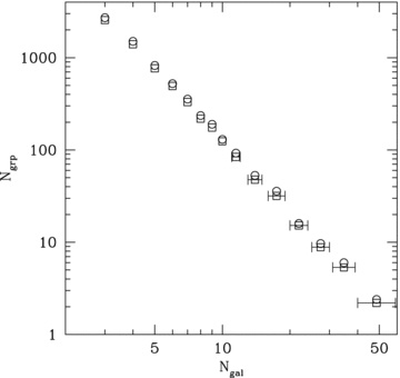
Galaxy group multiplicity function of SDSS Sample II. Circle points show the number of groups as a function of group richness, for groups with M≥ 10¹²h⁻¹ M_⊙ and ⁠. Square points show N_grp(N_gal) for groups in which we additionally require that the central galaxy is also the central galaxy of a group in Sample III. Horizontal error bars indicate the width of each bin.

Open in new tabDownload slide

The analysis of vdB05 was done with a catalogue of 2502 groups in the 2dFGRS with four members or more; the new Y07 catalogue has nearly twice as many groups with N_gal≥ 4 (4571), which is a significant improvement. In addition, the typical rms redshift and magnitude errors of galaxies in the SDSS are 30 km s⁻¹ and 0.035 mag (r band), respectively (Strauss et al. 2002), compared to 85 km s⁻¹ and 0.15 mag (B band) in the 2dFGRS (Colless et al. 2001). The improved statistics of this SDSS DR4 group catalogue allow us to investigate not only the halo mass dependence of central galaxy velocity bias, but also the dependence of velocity bias on the properties of the central galaxies themselves.

4 MOCK CATALOGUES

The main goal of this paper is to use the distributions of the parameters and defined above to test our three hypotheses related to the CGP defined in Section 1. As discussed above, since the SDSS galaxy group catalogue suffers from interlopers and incompleteness effects, we require mock group catalogues constructed from MGRSs using the same halo-based galaxy group finder as used for the SDSS.

We construct MGRSs by populating dark matter haloes with galaxies of different luminosities. The distribution of dark matter haloes is obtained from a set of large N-body simulations (dark matter only) for the 3-yr Wilkinson Microwave Anisotropy Probe (WMAP3) ΛCDM cosmology from Macciò et al. (2007). The simulations have 512³ particles each, have periodic boundary conditions, and have box sizes of L_box = 100 h⁻¹ Mpc (hereafter L₁₀₀) and L_box = 300h⁻¹ Mpc (hereafter L₃₀₀). We follow Yang et al. (2004) and replicate the L₃₀₀ box on a 4 × 4 × 4 grid. The central 2 × 2 × 2 boxes are replaced by a stack of 6 × 6 × 6 L₁₀₀ boxes (see fig. 11 in Yang et al. 2004). This stacking geometry circumvents incompleteness problems in the mock survey due to insufficient mass resolution of the L₃₀₀ simulations, and allows us to reach the desired depth of z_max = 0.20 in all directions.

Dark matter haloes are identified using the standard FOF algorithm with a linking length of 0.2 times the mean inter-particle separation. Unbound haloes and haloes with less than 10 particles are removed from the sample. The resulting halo mass functions are in excellent agreement with the analytical halo mass function of Sheth, Mo & Tormen (2001).

4.1 Assigning luminosities

We populate each halo with galaxies of different luminosities using the conditional luminosity function (CLF) model described in C09. The CLF, Φ(L|M), specifies the average number of galaxies of luminosity L in a halo of mass M, and is constrained to accurately match the SDSS r-band luminosity function (Blanton et al. 2003), the clustering strength of SDSS galaxies as a function of luminosity (Wang et al. 2007) and the galaxy–galaxy lensing data of Mandelbaum et al. (2006). The CLF assumes that the luminosity-dependent abundance, distribution and clustering of galaxies can be described as a function of halo mass. The CLF of C09 is split in two parts, Φ_cen(L|M) and Φ_sat(L|M), which describe the halo occupation statistics of central and satellite galaxies, respectively.

For each halo we draw the luminosity of its central galaxy from Φ_cen(L|M), which is parametrized as a lognormal distribution:

7

Here σ_cen = 0.14 quantifies the scatter between central galaxy luminosity and host halo mass. More et al. (2009) obtained a similar value from their analysis of satellite kinematics: σ_cen = 0.16 ± 0.04. The central galaxy luminosity as a function of halo mass, L_cen(M), is parametrized as a double power law, with a slope of 3.3 in low-mass haloes and 0.26 in massive haloes (see C09 for details).

For the satellite galaxies we assume that their halo occupation numbers follow a Poisson distribution with mean

8

where we adopt a luminosity threshold, L_min, corresponding to M_r− 5log h=−14. The satellite luminosities are drawn from the satellite CLF Φ_sat(L|M), which is parametrized as a modified Schechter function:

9

where ϕ_sat and α_sat are functions of halo mass, the parameter s = 2, and L*_sat (M) = 0.562 L_cen(M) (see C09 for details). We emphasize that this particular form for the CLF (equations 7 and 9) is not an assumption, but rather the form that agrees with the CLF obtained directly from the SDSS group catalogue (see Yang et al. 2008). The only poorly constrained parameter is s, and we test the effect of its uncertainty in Section 6.1.

If the luminosity of the satellite is brighter than that of its central, a new luminosity is drawn until it is fainter than that of the central. Hence, in our mock universe central galaxies are always BHGs by construction.

4.2 Assigning phase-space coordinates

Having assigned all mock galaxies their luminosities, the next step is to assign them a position and velocity within their halo.

We assume that each dark matter halo of mass M has a NFW (Navarro, Frenk & White 1997) density distribution, ρ_dm(r|M), with virial radius r_vir(M), characteristic scale radius r_s(M) and concentration parameter c(M) =r_vir/r_s. We model the halo concentrations using the c(M) relation of Macciò et al. (2007). Assuming haloes to be spherical and isotropic, the local, one-dimensional velocity dispersion follows from solving the Jeans equation

10

with Ψ(r) the gravitational potential (Binney & Tremaine 1987). Using that ∂Ψ/∂r=GM(r)/r² and defining the virial velocity we obtain

11

with f(x) = ln(1 +x) −x/(1 +x) and

12

The halo-averaged velocity dispersion is given by

13

(cf. van den Bosch et al. 2004).

4.2.1 Central galaxies

For the central galaxies, we proceed as follows. In the case of and mocks, we position the central galaxy at rest at the centre of the dark matter halo (for the mocks, we then reshuffle the indices of central and brightest satellite, as detailed below, but we do so only after the construction of the group catalogue). In the case of the mocks, we follow the approach of vdB05, to which we refer the reader for details. Briefly, we assume that the radial coordinate of the central, r, follows a probability distribution3

14

where a is a free parameter, which is related to the velocity bias b_vel as detailed below. In order to parametrize the characteristic radius a in terms of that of the dark matter halo, we define the parameter f_cen≡a/r_s.

Central galaxies in a halo of mass M at a halo-centric radius r have an isotropic velocity dispersion

15

with

16

This implies a halo-averaged velocity dispersion of

17

which allows us to define the velocity bias of central galaxies as

18

In addition to the velocity bias, we define the spatial bias as

19

where the expectation value for the radius follows from

20

For comparison, an NFW density distribution has 〈r|M〉 = 0.41r_vir(M) for c = 10, and 0.47r_vir(M) for c = 5.

With this model, a particular value of the parameter f_cen implies a particular amount of velocity and spatial bias. The relations b_vel(f_cen) and b_rad(f_cen) are shown in Fig. 2. These relations only depend weakly on halo concentration (see vdB05). In the limit f_cen→ 0, the probability distribution P_cen(r) becomes a delta function, implying that the central galaxy is sitting at rest at the centre of the dark matter halo (i.e. the null hypothesis of the CGP). Larger values of f_cen result in larger amounts of velocity and spatial bias. Note that b_vel is always larger than b_rad, indicating that the signature of an off-centred central galaxy (i.e. hypothesis ⁠) is more pronounced, and thus easier to detect, in velocity space than in configuration space.

Figure 2

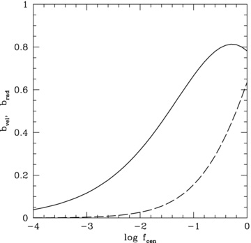
The velocity bias (solid curve) and spatial bias (dashed curve) of central galaxies as a function of the parameter f_cen, which expresses the characteristic scale of the radial distribution of central galaxies in terms of the characteristic scale of the NFW density distribution. The results shown correspond to a dark matter halo with a concentration c = 10.

Open in new tabDownload slide

4.2.2 Satellite galaxies

Throughout this paper, we assume that the N_sat satellite galaxies in a halo of mass M follow a number density distribution n_sat(r|M) = (N_sat/M)ρ_dm(r|M), so that there is no spatial bias between satellite galaxies and dark matter particles. If we further assume that the satellites are in isotropic equilibrium, it also follows that there is no velocity bias between the satellites and the dark matter, neither globally [i.e. 〈σ_sat|M〉=〈σ_dm|M〉] nor locally [i.e. σ_sat(r|M) =σ_dm(r|M)].

For simplicity, we assume that the satellites follow a spherically symmetric spatial distribution with a velocity distribution that is locally isotropic. Although this is a clear oversimplification, as some galaxy groups and clusters have anisotropic or aspherical distributions (e.g. Bailin et al. 2008; Wang et al. 2008), we do not believe that it strongly impacts our results. For example, the global velocity dispersion (i.e. obtained from all satellites) of an anisotropic system will be nearly identical to that of an isotropic system with the same gravitational potential, since both are governed by the virial equation. In other words, anisotropy changes the local line-of-sight velocity distribution (LOSVD), but leaves the second moment of the global LOSVD largely unchanged (see e.g. van den Bosch et al. 2004). Therefore, since the parameter (equation 4) only depends on the first and second moments of the global LOSVD, our results are robust to the assumptions of isotropy and sphericity. The cumulative -distribution is weakly dependent on higher moments of the LOSVD, but again, the effect of anisotropy is very small.

Although there is evidence to support our assumption that satellite galaxies have number density distributions that are well fit by a NFW profile (e.g. Lin, Mohr & Stanford 2004), the corresponding concentration parameters seem to be significantly smaller than the values expected for their dark matter haloes by about a factor of 2 to 3 (e.g. Hansen et al. 2005; Yang et al. 2005b). Since we assume that satellites are unbiased with respect to the dark matter, our value for b_vel will be incorrect by a factor of 〈σ_sat〉/〈σ_dm〉. Using the model described in equations (13) and (17), we estimate that this may result in an underestimating of the velocity bias by no more than 5 per cent. Given that this is a small effect compared to the other uncertainties involved in our analyses, we do not attempt to correct for it.

4.3 Mock group catalogues

Once the dark matter haloes are populated with galaxies, we construct an MGRS following the procedure described in Li et al. (2007). We place a virtual observer at the centre of the stack of simulation boxes, assign each galaxy a (α, δ)-coordinate and remove the ones that are outside the mocked SDSS survey region. For each model galaxy in the survey region, we compute its redshift (which includes the cosmological redshift due to the universal expansion, the peculiar velocity and a 35 km s⁻¹ Gaussian line-of-sight velocity dispersion to mimic the redshift errors in the data), and its r-band apparent magnitude (based on the r-band luminosity of the galaxy).

We eliminate galaxies that are fainter than the SDSS apparent magnitude limit, and incorporate the position-dependent incompleteness by randomly eliminating galaxies according to the completeness factors obtained from the survey masks provided by the NYU-VAGC (Blanton et al. 2005). Finally, we construct group catalogues from the MGRSs, using the same halo-based group finder as used for the real SDSS DR4.

Using the method outlined above, we construct the following set of mock group catalogues. The first is a set of 10 mocks that only differ in the value of the velocity bias b_vel = 0.0, 0.1, 0.2, 0.3, 0.4, 0.5, 0.6, 0.7, 0.8 and 1.0. These constitute our mocks. Note that the mock with b_vel = 0 satisfies the CGP, and therefore corresponds to the null hypothesis ⁠, while the other mocks correspond to (i.e. BHG is a central galaxy, but is not at rest at the centre of dark matter potential well). The second set of mock group catalogues is constructed starting from the b_vel = 0 mock group catalogue, in which we switch the luminosities of the central and its brightest satellite for a random fraction f_BNC of all groups. We construct six mock group catalogues for f_BNC = 0.1, 0.2, 0.3, 0.4, 0.5 and 0.6, respectively. These constitute our mocks.

In order to facilitate the comparison with the SDSS galaxy group catalogue, in what follows we discard all mock groups with an assigned group mass less than 10¹²h⁻¹ M_⊙, and with a satellite velocity dispersion or ⁠. For the mock groups that have not been discarded, we compute the parameters and ⁠. In the next section, we compare the resulting distributions and with those obtained from the SDSS group catalogue in order to test our three hypotheses ⁠, and ⁠.

Finally, we note that the halo centres and central and satellite galaxies are defined only in the mock group catalogues, not in the SDSS group catalogue. The and parameters used in the following analysis are defined with respect to the BHGs in the mock and observed galaxy groups. This way, we are able to statistically analyse groups of a wide range in mass, including poor groups for which a centre or central galaxy might not be well-defined.

5 RESULTS

Fig. 3 shows the cumulative distributions of (left panels) and (right panels) obtained from the mocks (upper panels) and the mocks (lower panels) for groups with four or more members (i.e. N_sat≥ 3). As expected, and become broader for larger values of b_vel (upper panels) and f_BNC (lower panels). A few trends are apparent. First, note that the -distributions are all bunched together for b_vel≤ 0.5. Only for b_vel > 0.5 are the cumulative -distributions notably different. This shows that it is difficult to constrain b_vel using the angular positions of galaxies, on which the -statistic is based, vis-à-vis using the velocity-statistic ⁠. Physically, this is a reflection of the fact that dark matter haloes have steep potential wells, so that large velocities are required even for relatively modest excursions from the centre. Secondly, and most importantly, comparing the upper and lower panels, it is clear that a non-zero value of f_BNC has a different impact on and than a non-zero value of b_vel. This is good news, as it implies that we will be able to discriminate between our three hypotheses.

Figure 3

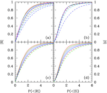
The cumulative distributions of (left-hand panels) and (right-hand panels) for the groups in mock group catalogues with four members or more. Upper panels show the distributions for mock catalogues with different amounts of b_vel: the solid curves are for b_vel = 0, 0.1, 0.2, 0.3 and 0.4 (red, green, magenta, cyan and blue curves, respectively, in the electronic version of this paper) and the dashed curves are for b_vel = 0.5, 0.6, 0.7, 0.8 and 1 (red, green, magenta, cyan and blue curves, respectively). Lower panels show the distributions for mock catalogues with different fractions f_BNC = 0, 0.1, 0.2, 0.3, 0.4, 0.5 and 0.6 (red, green, magenta, cyan, blue, dashed red and dashed green curves, respectively).

Open in new tabDownload slide

In what follows we will compare the cumulative and -distributions obtained from the SDSS with those obtained from our mock catalogues. Since we have a relatively large number of groups in our SDSS sample, we can perform this test for a (small) number of bins in group mass, thus giving some leverage on a possible halo mass dependence. At the massive end of the group mass distribution, the group catalogue is roughly complete, and the mass distribution closely follows the halo mass function. The constraint of four or more group members, however, cuts off the distribution at the low-mass end, leaving virtually no groups with M < 10¹²h⁻¹ M_⊙. We split the SDSS group catalogue in three mass bins (listed in Table 1) that contain a similar number (∼1500) of groups, and the corresponding mass cuts occur at log (M/h⁻¹ M_⊙) = 13.3 and 13.75.

Table 1

Open in new tab

Halo mass bins (log (M/h⁻¹ M_⊙)) in the SDSS group catalogue, for groups with four members or more and ⁠. The log mass ranges, mean masses, and number of groups are given.

Halo Mass Bins	log Mmin		log Mmax	Ngroup
low mass	12	12.86	13.3	1434
intermediate mass	13.3	13.53	13.75	1540
high mass	13.75	14.09	15.2	1555

Halo Mass Bins	log Mmin		log Mmax	Ngroup
low mass	12	12.86	13.3	1434
intermediate mass	13.3	13.53	13.75	1540
high mass	13.75	14.09	15.2	1555

Table 1

Open in new tab

Halo mass bins (log (M/h⁻¹ M_⊙)) in the SDSS group catalogue, for groups with four members or more and ⁠. The log mass ranges, mean masses, and number of groups are given.

Halo Mass Bins	log Mmin		log Mmax	Ngroup
low mass	12	12.86	13.3	1434
intermediate mass	13.3	13.53	13.75	1540
high mass	13.75	14.09	15.2	1555

Halo Mass Bins	log Mmin		log Mmax	Ngroup
low mass	12	12.86	13.3	1434
intermediate mass	13.3	13.53	13.75	1540
high mass	13.75	14.09	15.2	1555

The results presented in Sections 5.1 and 5.2 are based on groups with at least four members (i.e. with N_sat≥ 3). We have repeated these analyses using samples of groups with three, five, six, and 10 or more members. We have also tested lower and higher halo mass thresholds. In each case we obtain constraints on b_vel and f_BNC that are consistent with each other at the 1σ level. Hence, our results do not depend significantly on the multiplicity and halo mass thresholds used.

5.1 Testing hypothesis

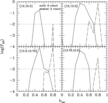
In order to test hypothesis ⁠, we compare the SDSS group catalogue to mock group catalogues with different values of b_vel while setting f_BNC = 0. Fig. 4(a) shows the cumulative -distribution for different bins of halo mass obtained from the SDSS group catalogue (solid lines) and from three mock group catalogues corresponding to different values of b_vel (0, 0.5 and 1). In all cases only groups with four members of more are considered. The numbers in square brackets in each panel indicate the range of log (M/h⁻¹ M_⊙) considered. Note that at fixed ⁠, the corresponding becomes smaller when using a bin with larger group masses. This does not necessarily imply a trend of b_vel with halo mass, though. It may also be due to a mass dependence of the fraction of interlopers, or a mass dependence of the completeness of group members. Indeed, the mock group samples for a fixed value of b_vel reveal the same trend, indicating that it is most likely an artefact introduced by the group finder. For each halo mass bin, the mock catalogue with b_vel = 0 (i.e. the one that fulfils the null hypothesis, ⁠, of the CGP) predicts an -distribution that is much narrower than that of the SDSS, while the mock catalogue with b_vel = 1 yields a distribution that is too broad. Interestingly, the intermediate case, with b_vel = 0.5, results in that are very similar to those of the SDSS, for each mass bin. This rules out the null hypothesis ⁠, and seems to suggest that instead central galaxies have a relatively large velocity bias with 〈σ_cen|M〉≃ 0.5〈σ_sat|M〉 with little dependence on halo mass M.

Figure 4

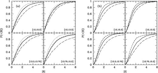
The cumulative distribution of (left-hand figure) and (right-hand figure) obtained from the SDSS group catalogue (solid black curve) compared with those obtained from three of our mocks, with b_vel = 0 (red dotted curve), 0.5 (blue short-dashed curve) and 1 (green long-dashed curve), for groups with four members or more. Results are shown for four log halo mass intervals, as indicated in square brackets in each panel.

Open in new tabDownload slide

However, Fig. 4(b), which is similar to Fig. 4(a) except that it shows the cumulative -distributions, paints a different picture. Both the b_vel = 0.0 and b_vel = 0.5 mocks predict -distributions that are clearly too narrow, for each mass bin. Rather, the SDSS -distribution seems to require 0.5 < b_vel < 1.0. Hence, it appears that no single value of b_vel can simultaneously match and obtained from the SDSS, ruling against our hypothesis ⁠. In other words, although the BHGs have non-zero velocities, the velocity spread is too small to explain their displacements from the halo centres.

In order to make this more quantitative, we use the Kolmogorov–Smirnov (KS) test to compute the probabilities P_KS that and of the SDSS and a particular mock are drawn from the same distribution. The results are shown in Fig. 5, which plots log (P_KS) as function b_vel for each of the four mass bins considered. Using the median and the 16 and 84 percentiles of P_KS(b_vel) for the distributions (solid lines) we obtain b_vel = 0.47^+0.06_−0.07 for the entire mass range, and b_vel = 0.44^+0.09_−0.07, b_vel = 0.50 ± 0.05 and b_vel = 0.43^+0.08_−0.06 for the low-, intermediate- and high-mass intervals, respectively. For the -distributions (dashed lines) this yields b_vel = 0.82^+0.08_−0.06 for the low-mass interval, and b_vel = 0.83^+0.08_−0.06 for the intermediate- and high-mass intervals. Therefore, the amounts of velocity bias consistent with the and -distributions of SDSS groups are significantly different, with their best-fitting values of b_vel differing from each other by more than 4σ. We conclude that hypothesis is ruled out, since it cannot simultaneously explain the and -distributions obtained from the SDSS group catalogue.

Figure 5

The KS-probability that the cumulative -distribution (solid lines) and -distribution (dashed lines) obtained from the SDSS groups is consistent with that obtained from our mocks, as a function of b_vel. Results are shown for four log halo mass intervals, indicated in square brackets in each panel. The horizontal dotted line in each panel indicates P_KS = 0.01: based on estimates of the scatter due to cosmic variance, we consider two distributions to be statistically equivalent when P_KS > 0.01.

Open in new tabDownload slide

5.2 Testing hypothesis

Having ruled out both and ⁠, we now turn our attention to hypothesis and investigate whether there is a value of f_BNC for which the mock group catalogue yields - and -distributions that are consistent with the SDSS data. To that extent we compare the SDSS group catalogue to mock catalogues with b_vel = 0, but with different values of f_BNC. We proceed in the same way as for in the previous section: for each mock, which corresponds to a different value of f_BNC, we compute and ⁠, which we compare to the corresponding distributions obtained from the SDSS, resulting in a value for P_KS, the KS-probability that the mock and SDSS distributions are consistent with each other.

The results are shown in Fig. 6, where the solid and dashed lines once again correspond to the and -distributions, respectively. These KS probabilities are the means of log(P_KS) for 100 realizations with different random seeds. The solid lines show that the -distribution of SDSS groups indicates a relatively large fraction of groups in which the central galaxy is not the BHG, with f_BNC increasing from ∼0.25 in low-mass haloes (10¹²h⁻¹ M_⊙≤M≲ 2 × 10¹³h⁻¹ M_⊙) to ∼0.4 in massive haloes (M≳ 5 × 10^13.75h⁻¹ M_⊙). Interestingly, the KS probabilities obtained from the -distributions shown by the dashed lines yield best-fitting values of f_BNC that are very similar. Hence, we conclude that contrary to hypothesis ⁠, hypothesis can simultaneously match the and obtained from the SDSS group catalogue.

Figure 6

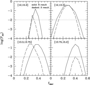
The KS-probability that the cumulative -distribution (left-hand figure) and -distribution (right-hand figure) obtained from the SDSS groups with four or more members is consistent with that obtained from MGRSs, as a function of f_BNC, the fraction of groups in which the most luminous satellite is brighter than the central galaxy (see text for details). The KS probabilities here are the means of log(P_KS) for 100 realizations with different random seeds.

Open in new tabDownload slide

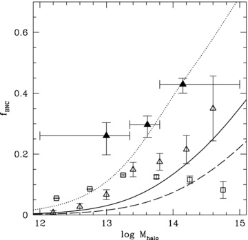
Fig. 7 summarizes our results. It shows the best-fit values of b_vel (upper panel) and f_BNC (lower panel) as functions of halo mass, as inferred from the -distributions (squares) and -distributions (triangles) obtained from the SDSS galaxy group catalogue. The figure clearly shows that (i.e. a non-zero f_BNC) can simultaneously explain both the velocities and the positions of BHGs with respect to their satellites, while (i.e. a non-zero b_vel) is ruled out because it cannot.

Figure 7

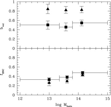
Halo mass dependence of b_vel (upper panel) and f_BNC (lower panel), inferred from the -distributions (squares) and -distributions (triangles) obtained from the analyses of the SDSS group catalogue (see the text for details). For the results in the upper panel, the mock catalogues had different values of b_vel and f_BNC = 0; for the lower panel, the mocks had different values of f_BNC and b_vel = 0. Points show best-fitting values of the parameters estimated from the KS probabilities; vertical error bars show 1σ uncertainties from the 16 and 84 percentiles of the P_KS-distributions and horizontal error bars indicate the widths of the mass bins. Hypothesis is clearly ruled out from the fact that the -data imply a velocity bias, b_vel, that is inconsistent with the value inferred from the -data.

Open in new tabDownload slide

Considering the - and -distributions simultaneously, we infer best-fitting values for the fraction of haloes in which centrals are not BHGs of f_BNC = 26⁺⁴₋₆ per cent for 12 ≤ log (M/h⁻¹ M_⊙) < 13.3, increasing to f_BNC = 30⁺³₋₄ per cent for haloes with 13.3 ≤ log (M/h⁻¹ M_⊙) < 13.75 and f_BNC = 43⁺²₋₃ per cent in the most massive haloes with log (M/h⁻¹ M_⊙) ≥ 13.75. As in Section 5.2, the best-fitting values and uncertainties are determined from the median and the 16 and 84 percentiles of the P_KS(f_BNC)-distributions.

Before proceeding with a discussion regarding the implications of these findings, we briefly address the possibility that both and are true; BHGs are not central galaxies in a non-zero fraction f_BNC of all haloes, and central galaxies have a non-zero value for their velocity bias b_vel. Using mock group catalogues with non-zero values for both f_BNC and b_vel we estimate that the data can accommodate a small amount of velocity bias b_vel≲ 0.2. We emphasize, though, that the data do not require a non-zero b_vel.

5.3 The impact of substructure

In the tests described above, we have always assumed that satellite galaxies follow a smooth, spherically symmetric, number density distribution, and we assigned the satellites’ peculiar velocities within its host halo under the assumption that the corresponding potential is smooth. This ignores the fact that dark matter haloes are believed to have a wealth of substructure (see Giocoli et al. 2010, and references therein; on substructure in galaxy clusters, see Richard et al. 2010). Satellite galaxies are believed to be associated with these substructures. Our treatment of the spatial and kinematic properties of satellite galaxies is only consistent with this concept of substructure if: (i) each subhalo hosts at the most one satellite, and (ii) the positions and velocities of subhaloes are not correlated with those of other subhaloes. In reality, neither of these criteria is likely to be met. Massive subhaloes are likely to host multiple satellites, and the large-scale filamentary structure is believed to introduce (weakly) correlated directions of infall for subhaloes (e.g. Vitvitska et al. 2002; Aubert, Pichon & Colombi 2004; White, Cohn & Smit 2010). Both of these effects result in correlations among the positions and/or velocities of different satellite galaxies within the same host halo, which is likely to have an impact on the and statistics.

In order to have a crude estimate of the impact of substructure, we proceed as follows. We start by populating 1000 (virtual) dark matter haloes, all with M = 3 × 10¹⁴h⁻¹ M_⊙, with galaxies using the same CLF model as in Section 4. Similar to the mocks, we assure that the central galaxy is always the brightest galaxy in the halo, and we position it at rest at the centre of the halo. We then compute and for each of these haloes. The black, solid lines in Fig. 8 indicate the corresponding and ⁠. Next we repeat this exercise, but now, in each halo, a fraction f_sub of all satellites is ‘clumped’ together in a single substructure. We model this substructure as a halo of mass m=f_subM (i.e. we assign the galaxies in this subhalo phase-space coordinates in exactly the same way as we would if the halo was a ‘host’ halo of the same mass). The phase-space coordinates of the centre of the subhalo are drawn in the same way as the phase-space coordinates of the satellites that are not in a substructure. The long-dashed green curves, short-dashed blue curves and dotted red curves in Fig. 8 show the and thus obtained for f_sub = 1/3, 1/5 and 1/10, respectively. A comparison with the no-substructure case (black, solid line) shows that substructure significantly affects the and -distributions, and hence our conclusions, if all dark matter haloes have a most massive substructure whose mass is m_sub≳ 0.1M. In particular, if many haloes contain substantial substructure, then an alternative explanation for the fact that our fiducial model (which follows the CGP) does not match the data may be that the phase-space coordinates of satellite galaxies within the same dark matter host halo are correlated. In that case the fractions f_BNC obtained in Section 5.2 will be significantly overestimated.

Figure 8

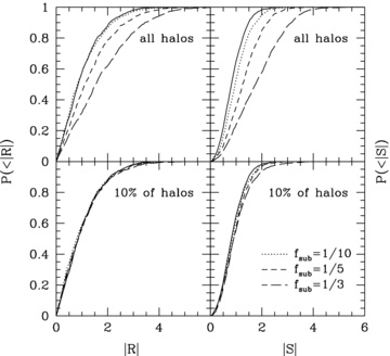
Cumulative distributions of (left-hand panels) and (right-hand panels) of 1000 mock haloes with M = 3 × 10¹⁴h⁻¹ M_⊙ populated with galaxies. Black solid curves indicate the distributions for haloes with no substructure, while the long-dashed green curves, short-dashed blue curves and dotted red curves indicate the distributions for f_sub = 1/3, 1/5 and 1/10, respectively. Results are shown for the case in which all haloes have substructure (upper panels) and 10 per cent of the haloes have substructure (lower panels).

Open in new tabDownload slide

However, using the subhalo mass functions of Giocoli et al. (2010), we estimate that only ∼8 per cent of host haloes with M = 3 × 10¹⁴h⁻¹ M_⊙ have a most massive subhalo with f_sub=m/M≥ 0.1, while only ∼0.7 per cent have a most massive subhalo with m/M≥ 0.3. Based on these estimates, and on the tests described above, we argue that ignoring substructure when populating haloes with (satellite) galaxies does not have a significant impact on the and statistics, though more sophisticated tests are required to confirm this. Therefore, we conservatively argue that the f_BNC fractions obtained in this paper have to be regarded as upper limits.

6 DISCUSSION

The results presented in the previous section suggest that in as much as 25 to 40 per cent of all haloes, the brightest galaxy is a satellite rather than a central galaxy. In order to put these numbers in perspective, we compare them to predictions from halo occupation statistics (Section 6.1) and from two semi-analytical models (SAMs) of galaxy formation (Section 6.2). We also investigate the impact of non-zero f_BNC(M) on the halo masses inferred using satellite kinematics (Section 6.3).

6.1 Comparison with halo occupation statistics

Using the SDSS r-band luminosity function of Blanton et al. (2003), the projected two-point correlation functions of Wang et al. (2007) and the galaxy–galaxy lensing data of Mandelbaum et al. (2006), C09 constrained the halo occupation statistics as parametrized by the CLF

21

which is found to be in good agreement with direct constraints from the Y07 group catalogue (Yang, Mo & van den Bosch 2008; Yang et al. 2009a) and with constraints from satellite kinematics (More et al. 2009). We have used this CLF model in Section 4.1 to construct our mock group catalogues, except that we imposed that the central galaxy is always the BHG; if a satellite luminosity was drawn from Φ_sat(L|M) that was brighter than the central luminosity, drawn from Φ_cen(L|M), it was rejected. Later, we then switched the luminosities of the central and that of its brightest satellite in a fraction f_BNC of all groups. We now use the CLF to ‘predict’ the fraction f_BNC as function of halo mass, by making the assumption that the luminosities of satellite galaxies are independent of the luminosity of the central galaxy in the same halo. In that case, the probability that a random satellite galaxy in a halo of mass M has a luminosity smaller than that of its central is simply given by

22

where the integral accounts for the scatter in the relationship between central galaxy luminosity and halo mass, and L_min is the minimum luminosity considered. In a halo with N_sat satellites, the probability that the central galaxy is also the brightest galaxy is simply ⁠. Hence, we obtain that

23

where P(N_sat|M) gives the probability that a halo of mass M contains N_sat satellites, which we take to be a Poisson distribution whose mean is given by equation (8). The results thus obtained from the CLF of C09 are shown as a solid line in Fig. 9. For comparison, the solid triangles with error bars are the constraints on f_BNC(M) obtained from the SDSS group catalogue as described in the previous section. Although the CLF predicts that f_BNC increases with increasing halo mass, in qualitative agreement with the data, the values of f_BNC(M) inferred from the data are much larger than those ‘predicted’ by the CLF. Note that the CLF prediction is for all haloes, rather than for haloes (or groups) with N_sat≥ 3, which is the richness threshold used in our analysis of SDSS groups. However, this has little to no impact. We have verified that our constraints on f_BNC do not change significantly if we use a different richness threshold. Furthermore, from the CLF, the probability of a halo hosting fewer than three galaxies is low for most of the mass range considered here: P(N_sat < 3) > 0.05 only for haloes with logM < 12.75.

Figure 9

Probability that the most luminous satellite galaxy is brighter than the central galaxy in a halo, as a function of halo mass (equation 23). Result is shown for three slopes in the satellite CLF (equation 9): s = 1 (dotted curve), the fiducial s = 2 (solid curve) and s = 3 (dashed curve). For comparison, the f_BNC(M_halo) result from Fig. 7 (solid triangle points) is also shown. The predictions from the morgana semi-analytic model (open triangles) and Croton et al. (2006) semi-analytic model (open squares) are also shown, with Poisson errors.

Open in new tabDownload slide

There are a number of possible explanations for why the CLF prediction is not consistent with the data. First of all, we emphasize that the CLF is not designed to ‘predict’ f_BNC(M). Most of the statistics used to constrain the CLF depend only very weakly (clustering and lensing) or not at all (luminosity function) on f_BNC(M). Secondly, it is still possible that the CLF is correct, but that the additional assumption that the satellite luminosity is independent of the luminosity of the central is not correct, that is Φ_sat(L_sat|M, L_cen) ≠Φ_sat(L_sat|M). This could come about, for example, because of galactic ‘cannibalism’: those haloes in which the central has recently cannibalised a bright satellite will have an excessively bright central, and are less likely to have a bright satellite. It remains to be seen whether a model for Φ_sat(L_sat|M, L_cen) can be found that yields a f_BNC(M) in better agreement with the data, and simultaneously obeys the CLF constraint that

24

Of course, it is also possible that the discrepancy reflects an actual failure of the CLF. One possible modification, which will have little impact on the luminosity function, clustering, galaxy–galaxy lensing and mock group catalogues is a modification in the shape of Φ_sat(L|M) (equation 9) at the bright end. As mentioned in Section 4.1, C09 adopted a functional form for which Φ_sat(L|M) ∝ exp [− (L/L*_sat)^s] at the bright end, with s = 2. The exact value of s, though, is poorly constrained by the data, but has a significant impact on f_BNC(M). This is illustrated by the dotted and dashed curves in Fig. 9, which correspond to s = 1 and s = 3, respectively. Clearly, decreasing s increases the expectation value for the luminosity of the brightest satellite, and hence the fraction of haloes for which the central galaxy is not the BHG. For s = 1 the CLF ‘predicts’ a f_BNC(M) in good agreement with the data, but only for M≳ 5 × 10¹³h⁻¹ M_⊙. For less massive haloes, the value of f_BNC inferred from the SDSS group catalogue is still too high compared to the CLF prediction, but only by about 2σ.

Another parameter that has a significant impact on f_BNC(M) is the ratio Q≡L*_sat/L_cen. Motivated by the CLF inferred from the SDSS group catalogue by Yang et al. (2008), C09 adopted Q = 0.562, with no dependence on halo mass. However, Hansen et al. (2009), using the maxBCG group catalogue of Koester et al. (2007), found that Q depends on halo mass and may be as small as ∼0.15 for M∼ 10¹⁴h⁻¹ M_⊙. In order for the CLF to yield f_BNC(M) in rough agreement with our findings, though, we need a value of Q that is larger than 0.562 (i.e. for s = 2 we require Q∼ 0.7). These results warrant a more thorough investigation into the exact values of s and Q as function of halo mass.

Finally, we have verified that the CLF predictions for f_BNC(M) do not depend significantly on our choice for the lower luminosity cut-off, L_min.

6.2 Comparison with semi-analytical models

We now compare our results to the predictions of two SAMs of galaxy formation; the MORGANA model of Monaco, Fontanot & Taffoni (2007), as updated by Lo Faro et al. (2009), and the SAM of Croton et al. (2006).

Both SAMs adopt flat ΛCDM cosmologies, albeit with slightly different values for the cosmological parameters.4 Although both SAMs include treatments of cooling, star formation, feedback from supernovae and active galactic nuclei, mergers, starbursts and disc instabilities, the actual implementations of these physical processes are substantially different (see the original papers for details). Yet, as shown in Fig. 9 (open symbols), they predict fairly similar values for f_BNC(M).5 In qualitative agreement with the data, both SAMs predict that f_BNC increases with halo mass. In addition, from studying the satellite BHGs in the MORGANA model, we find that the majority of the more massive satellites represent a recently (since z∼ 0.2) accreted population, in most cases linked to the last major merger experienced by the host halo. In other words, infalling massive satellites could be a contributing cause of a non-zero f_BNC.

As with the halo occupation statistics, the predictions of both models are significantly lower than the data. In both SAMs, satellite galaxies are ‘strangulated’ after being accreted by their host galaxies, so that they do not participate in the cooling flow of their parent halo. However, it has been pointed out that the standard, instantaneous implementation of this strangulation causes an overquenching of satellite galaxies (e.g. Baldry et al. 2006; Weinmann et al. 2006; Kimm et al. 2009). It has been suggested that this overquenching problem can be avoided by adopting a longer time-scale for strangulation (e.g. Kang & van den Bosch 2008; Font et al. 2008; Weinmann et al. 2009). This is likely to allow satellite galaxies to continue forming stars for some period, which will increase their stellar mass, and thus also f_BNC. The effect, though, is likely to be small. Another effect that may cause the SAMs to underpredict f_BNC is the fact that they often adopt dynamical friction time-scales that are too short (Boylan-Kolchin, Ma & Quataert 2008; Wetzel & White 2010). This results in (massive) satellites being accreted too rapidly, and hence in an underestimate of f_BNC. Finally, the models do not take proper account of stellar mass stripping due to tidal forces, which will make satellites less massive. As emphasized in a number of recent papers, this tidal stripping of satellite galaxies is an important ingredient of galaxy formation (Monaco et al. 2006; White et al. 2007; Conroy, Ho & White 2007; Conroy, Wechsler & Kravtsov 2007; Kang & van den Bosch 2008 ; Yang, Mo & van den Bosch 2009b; Pasquali et al. 2010). It remains to be seen to what extent these additions and/or modifications of the SAMs impact f_BNC(M). For the moment, we conclude that the f_BNC(M) inferred from our analysis of SDSS galaxy groups is uncomfortably high compared to predictions from both halo occupation statistics and SAMs of galaxy formation.

6.3 Implication for satellite kinematics

Studies that attempt to infer the masses of dark matter haloes using the kinematics of satellite galaxies always assume that the CGP is valid (e.g. Zaritsky et al. 1993; McKay et al. 2002; van den Bosch et al. 2004; More et al. 2009). Since a typical central only has a few satellites, one normally stacks many centrals together in order to obtain sufficient signal-to-noise ratio to measure a reliable satellite velocity dispersion, σ_sat. With sufficiently large galaxy redshift surveys, one can measure σ_sat as a function of the luminosity (or stellar mass) of the central galaxies (i.e. one stacks centrals in narrow bins in luminosity or stellar mass).

Consider a halo with N_sat satellites with velocities v_{sat, i} with respect to halo centre, and let the central be stationary at the centre of the halo (i.e. v_cen = 0). The satellite velocity dispersion measured with respect to the central is

25

Without loss of generality, assume that satellite number 1 is misidentified to be the central. The measured velocity dispersion in this case will be

26

The first term sums over the remaining N_sat− 1 true satellites, while the last term is the contribution from the true central. Using that 〈v_{sat, i}〉 = 0, and that 〈v_cen〉=〈v²_cen〉 = 0, it is easy to show that the velocity dispersion measured from a stack of many systems, each with N_sat satellites, is equal to

27

where f_BNC is the fraction of systems in which the central is misidentified. Note that when the number of satellites per central is one, the measured velocity dispersion is identical to the true one, independent of f_BNC, that is the fact that some satellites are misidentified as centrals has no impact on the inferred satellite kinematics.6 However, in the limit N_sat→∞, one has that ⁠. Since the inferred halo mass M∝σ³_sat, this implies that the mass of the halo will be overestimated by a factor (1 +f_BNC)^3/2. Note that equation (27) is strictly valid only for stacks of systems that all have the same number of satellites. In reality, however, there will be scatter in the number of satellites per host in the stack. In what follows we assume that we do not make a large error if we adopt equation (27) but with N_sat replaced by the average number of satellites per central, 〈N_sat〉.

For relatively faint centrals, 〈N_sat〉≃ 1, and σ_meas≃σ_true independent of the value of f_BNC. However, at the bright end 〈N_sat〉 becomes substantially larger than unity, and a non-zero f_BNC may cause a significant overestimate of the true σ_sat. For example, in their analysis of satellite kinematics, More et al. (2009) have 〈N_sat〉∼ 10 for their brightest host bins. If f_BNC for these bins is comparable to f_BNC(M) at the massive end (i.e. f_BNC∼ 0.4), their inferred halo masses around bright host galaxies will be overestimated by a factor of ∼1.6.

However, since the halo mass luminosity relation for central galaxies is not one-to-one, it is not trivial to infer f_BNC for a certain bin in host galaxy luminosity, L_host, from f_BNC(M). In fact, one can construct mocks in which f_BNC(L_host) is very small at the bright end, even when f_BNC(M) is large at the massive end, by making the criterion for a halo having a satellite brighter than the central conditional on the luminosity of the central galaxy. We illustrate a particular case of this in Fig. 10, where we show f_BNC(L_BHG) for two types of mocks that have identical f_BNC(M) = 0.4. These are constructed as follows. We start by populating the dark matter haloes in our 100h⁻¹ Mpc simulation box described in Section 4 with galaxies of different luminosities using the CLF of C09 (see Section 4.1 for details). If the luminosity of a satellite is brighter than that of its central, a new luminosity is drawn until it is fainter than that of the central, so that f_BNC = 0. For the first set of mocks, we switch the luminosities of the central and that of its brightest satellite in a random fraction of 40 per cent of all haloes, and we measure the resulting f_BNC(L_BHG). We refer to these as the ‘random’ mocks. The mean and scatter obtained from 10 realizations are shown as the solid line in Fig. 10. As expected, f_BNC(L_BHG) ≃ 0.4, independent of L_BHG. For the second set of mocks, we again start from the mocks with f_BNC = 0, but we now switch the luminosities of brightest satellite and central in those haloes that meet the criterion

28

that is in those haloes in which the luminosity of the central falls in the lower 40 percentile of its distribution, Φ_cen(L|M). We refer to these as the ‘conditional’ mocks, and similar to the ‘random’ mocks they thus have f_BNC(M) = 0.4. Yet, their f_BNC(L_BHG), indicated by the dotted curve in Fig. 10, are very different: they decrease from ∼0.4 at the faint end to almost zero at the bright end. Hence, if the probability that a central is not the BHG is conditional on the luminosity of the central, which seems to be a reasonable assumption, then even a relatively large f_BNC(M) may have negligible impact on the halo masses inferred from satellite kinematics.

Figure 10

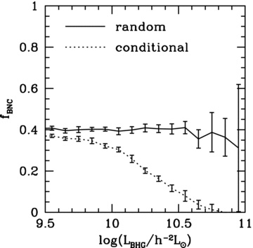
Fraction f_BNC of haloes in which the brightest galaxy is not the central one, as a function of the luminosity of the BHG. The solid line shows f_BNC(L_BHG) for the ‘random’ mocks, and the dotted line shows the fraction for the ‘conditional’ mocks, in which whether a halo has a satellite brighter than the central is conditional on the luminosity of the central galaxy. The luminosities correspond to r-band absolute magnitudes, such that log L = 9.5 corresponds to M_r≈−19, and log L = 10.3 to M_r≈−21, etc.

Open in new tabDownload slide

We thus conclude that a proper assessment of the impact of a non-zero f_BNC(M) on the halo masses inferred from satellite kinematics requires an independent assessment of the fraction f_BNC as function of the luminosities of the host galaxies.

7 CONCLUSIONS

It is generally assumed that the central galaxy in a dark matter halo, that is the galaxy with the lowest specific potential energy, is also the BHG and that it resides at rest at the centre of the dark matter potential well. This CGP is an essential assumption made in various fields of astronomical research (e.g. satellite kinematics, gravitational lensing, both weak and strong, halo occupation modelling).

In this paper, we have used a large galaxy group catalogue, constructed from the SDSS DR4 by Y07, in order to test the validity of the CGP. For each group we compute two statistics, and ⁠, which quantify the offsets of the line-of-sight velocities and projected positions of brightest group galaxies relative to the other group members. By comparing the cumulative distributions of and to those obtained from detailed mock group catalogues, we have tested the null hypothesis, ⁠, that the CGP is correct; hypothesis ⁠, according to which central galaxies are BHGs but have a non-zero velocity with respect to the halo centre, parametrized by a non-zero velocity bias, b_vel; and hypothesis ⁠, according to which central galaxies reside at rest at the centre of the halo’s potential well, but are not the BHGs in a fraction f_BNC of all haloes.

In agreement with vdB05, who only used the statistic, we show that the null hypothesis is strongly ruled out. However, contrary to vdB05, who argued that the data are consistent with a non-zero b_vel, we show that fails to simultaneously match the and -distributions.7 Rather, we have shown that the data are consistent with hypothesis ⁠, indicating that BHGs are not central galaxies in a non-negligible fraction of all haloes; in particular, we find that f_BNC increases from ∼0.25 in low-mass haloes (10¹²h⁻¹ M_⊙≤M≲ 2 × 10¹³h⁻¹ M_⊙) to ∼0.4 in massive haloes (M≳ 5 × 10¹³h⁻¹ M_⊙).

Considering combined models, in which BHGs are not central galaxies in a non-zero fraction f_BNC of all haloes, and central galaxies have a non-zero value for their velocity bias b_vel, we find that the data can at most accommodate a small amount of velocity bias (b_vel≲ 0.2). We emphasize, though, that a non-zero velocity bias is not required by the data (see vdB05 for a discussion of possible physical explanations for a non-zero b_vel).

Our main result is that the fraction f_BNC is significant and increases with halo mass. Since some authors have assumed that the most luminous (or most massive) galaxy in a system is the central galaxy, our result that f_BNC is somewhat large in galaxy groups and larger (43⁺²₋₃ per cent) in more massive clusters may seem surprising. Nevertheless, our results are consistent with other studies. For example, von der Linden et al. (2007) find that in 343 of their 625 clusters (≈55 per cent), the identified BCG is not the ‘mean’ galaxy (which lies at the centre of the cluster’s density field). Coziol et al. (2009) find that in about half of their 452 clusters, the BCGs have a median peculiar velocity greater than one third of their clusters’ velocity dispersion. Finally, in the Local Group, although the MW and Andromeda both have their own systems of satellites, they could be considered part of a single group, in which Andromeda would be identified as the BHG (van den Bergh 1999). The two galaxies are expected to eventually merge, although neither is clearly the ‘central’ galaxy.

In order to put our constraints on f_BNC(M) in perspective, we have compared them to predictions from SAMs for galaxy formation and from halo occupation statistics. Both the SAM of Croton et al. (2006) and that of Lo Faro et al. (2009) predict 0.1 ≲f_BNC≲ 0.2 in the halo mass range of 10¹³h⁻¹≲M≲ 10¹⁵h⁻¹ M_⊙, significantly lower than the f_BNC(M) inferred here from our SDSS galaxy group catalogue.

We can also use the CLF model of C09 to predict f_BNC(M), if we assume that the luminosity of a satellite galaxy is independent of the luminosity of its corresponding central. Although the C09 halo occupation model accurately matches the SDSS r-band luminosity function of Blanton et al. (2003), the projected two-point correlation functions of Wang et al. (2007) and the galaxy–galaxy lensing data of Mandelbaum et al. (2006), this model also predicts a f_BNC(M) that is far too low. We have shown that one can increase the predicted f_BNC(M) using some small modifications of the CLF, but it remains to be seen how these modifications impact the clustering and lensing predictions. For completeness, we emphasize that halo occupation models based on the abundance-matching method (e.g. Vale & Ostriker 2004; Conroy, Wechsler & Kravtsov 2006; Conroy et al. 2007; Shankar et al. 2006; Guo et al. 2010; Moster et al. 2010) ‘predict’ that f_BNC = 0, by construction, unless they assume a non-zero scatter in the relation between central galaxy luminosity and halo mass. Typically a larger amount of scatter will imply a larger f_BNC. It remains to be seen whether the amount of scatter required to match the f_BNC(M) inferred here is consistent with independent constraints, such as those obtained from satellite kinematics (More et al. 2009). All in all, we conclude that the constraints on f_BNC(M) obtained in this paper are uncomfortably high compared to predictions from galaxy formation models and halo occupation statistics. One possible explanation may be that dark matter haloes have substructure, something that we have ignored in our analysis. Although simple tests suggest that the correlations in the phase-space parameters of satellite galaxies due to substructure are not strong enough to significantly impact our conclusions, we caution that more detailed studies are required to confirm this.

Our results have important implications for various areas in astrophysics. In particular, we have shown that a non-zero f_BNC may cause an overestimate of halo masses inferred from satellite kinematics. Although the effect is expected to be negligible for faint host galaxies, because they typically only have of the order of one satellite per host, the overestimate can be significant at the bright end. The exact impact, though, depends on the fraction f_BNC as function of the host luminosity, which may be very different from that as a function of halo mass. For example, if BHGs are not centrals in the fraction f_BNC(M) of haloes of mass M that host the faintest centrals, then f_BNC(L) drops towards zero at the bright end, and the impact on satellite kinematics is negligible.

Additional methods and analyses that may be affected by a non-zero f_BNC are the following.

• The inference of halo masses from weak gravitational lensing. Similar to satellite kinematics, weak lensing studies often rely on stacking the lensing signals of many clusters and groups binned by mass-correlated observables such as richness and luminosity. When interpreting such data, it is generally assumed that BHGs coincide with the centres of the dark matter haloes (e.g. Mandelbaum et al. 2006; Johnston et al. 2007; Sheldon et al. 2009a,b; Corless & King 2009; C09). Since satellite galaxies yield a different lensing signal than centrals, at least on small to intermediate scales (see e.g. Yang et al. 2006), a non-zero f_BNC may have a significant impact on the lensing signal (Johnston et al. 2007), by resulting in underestimates of the richnesses and lensing profiles, for example. C09 used the CLF described in Section 4.1 to model the galaxy–galaxy lensing signal of Mandelbaum et al. (2006). As shown in Section 6.1, this CLF predicts f_BNC(M) significantly lower than inferred here. It remains to be seen to what extent this may affect their interpretation of the lensing data.

• Analyses of the power spectrum of luminous red galaxies (Tegmark et al. 2006; Reid et al. 2010), which can be used to constrain cosmological parameters. In tests with mock galaxy catalogues, Reid et al. (2010) find that a fraction f_BNC of 0.2–0.4 results in an angle-averaged LRG power spectrum that is damped by 2–4 per cent on scales of k∼ 0.1 h Mpc⁻¹, and the effect is larger at larger k. However, when analysing the observed power spectrum with these mock catalogues, the effect of f_BNC on the recovered cosmological parameters is relatively small.

• Measurements of the radial number density distribution of satellite galaxies, n_sat(r|M), in haloes of mass M. Several studies that have measured n_sat(r|M) using groups and clusters have assumed that the halo centre coincides with the location of the BHG (e.g. Carlberg, Yee & Ellingson 1997; Collister & Lahav 2005; Hansen et al. 2005; Yang et al. 2005b). If, instead, the BHG is a satellite galaxy, this will result in an underestimate of the concentration of n_sat(r). Hence, a non-zero f_BNC(M) may cast doubt on the claim, made by several of these studies, that satellite galaxies are less centrally concentrated than the dark matter. On the other hand, Lin et al. (2004) used the centre of the X-ray emission as the centre of the dark matter halo, rather than the location of the BHG, and came to a similar conclusion.

• Comparisons of the properties of central and satellite galaxies. A number of recent studies have used galaxy group catalogues to split the galaxy population into centrals and satellites, and to compare their properties (e.g. Weinmann et al. 2006, 2009; Skibba et al. 2007; van den Bosch et al. 2008; Pasquali et al. 2009, 2010; Hansen et al. 2009; Kimm et al. 2009; Skibba 2009; Guo et al. 2009). Since all of these studies have assumed the brightest group galaxy to be the central galaxy, they are likely to have underestimated the true differences (i.e. a non-zero f_BNC blurs the actual differences between centrals and satellites).

We thank Darren Croton for making the results from his SAM available to us in electronic format, and Eric Bell, Kris Blindert, Romeel Davé, Xi Kang, Tod Lauer, Alexie Leauthaud, Pierluigi Monaco, Beth Reid, Maria Pereira, Simone Weinmann and Ann Zabludoff for valuable discussions about our results and their implications. Some of the calculations were carried out on the PIA cluster of the Max-Planck-Institute für Astronomie at the Rechenzentrum Garching.

REFERENCES