


Abstract
We present a wide-field Integral Field Spectroscopy (IFS) survey on the nearby face-on Sbc galaxy NGC 628, comprising 11094 individual spectra, covering a nearly circular field-of-view of ∼6 arcmin in diameter, with a sampling of ∼2.7 arcsec per spectrum in the optical wavelength range (3700–7000 Å). This galaxy is part of the PPAK IFS Nearby Galaxies Survey (PINGS). To our knowledge, this is the widest spectroscopic survey ever made in a single nearby galaxy. A detailed flux calibration was applied, granting a spectrophotometric accuracy of ∼0.2 mag. The spectroscopic data were analysed both as a single integrated spectrum that characterizes the global properties of the galaxy and using each individual spectrum to determine the spatial variation of the stellar and ionized gas components. The spatial distribution of the luminosity-weighted ages and metallicities of the stellar populations was analysed. Using typical strong emission-line ratios we derived the integrated and 2D spatial distribution of the ionized gas, the dust content, star formation rate (SFR) and oxygen abundance.
The age of the stellar populations shows a negative gradient from the inner (older) to the outer (younger) regions. We found an inversion of this gradient in the central ∼1 kpc region, where a somewhat younger stellar population is present within a ring at this radius. This structure is associated with a circumnuclear star-forming region at ∼500 pc, also found in similar spiral galaxies. From the study of the integrated and spatially resolved ionized gas, we found a moderate SFR of ∼2.4 M⊙ yr−1. The oxygen abundance shows a clear gradient of higher metallicity values from the inner part to the outer part of the galaxy, with a mean value of 12 + log(O/H) ∼ 8.7. At some specific regions of the galaxy, the spatially resolved distribution of the physical properties shows some level of structure, suggesting real point-to-point variations within an individual H ii region. Our results are consistent with an inside–out growth scheme, with stronger star formation at the outer regions, and with evolved stellar populations in the inner ones.
1 INTRODUCTION
Galaxies in the local universe (∼10 Mpc) are the fundamental anchor points of any study of the evolution of these objects in cosmological time-scales. Therefore, it is important to understand their main properties, including their morphology, ionized and neutral gas content, stellar populations and metallicities. Due to their apparent scalelength, they represent the perfect laboratories to study the dependence of the stellar population, the star formation history (SFH) and star formation rate (SFR) on the morphology and morphological substructures, the metallicity enrichment and the mechanisms of metal transfer, as well as the nature of the gas ionization.
Powerful constraints on theories of galactic chemical evolution, on the SFH and on the nucleosynthesis in galaxies can be derived from the accurate determination of the nature of the ionization, the SFR and the chemical abundances at different locations within a galaxy. Fortunately, these sort of studies can be addressed using ground-based astronomy by observing galaxies with large apparent scalelengths. Nearby galaxies may be more easily separated into a number of different morphological components and several types of stellar populations. Given the spatial variation in the star formation histories (including violent episodes in some cases), and the amount of dust attenuation within a galaxy, and their relatively low surface brightness, it is difficult to study the stellar populations of nearby galaxies using just their integrated light. More information can be extracted by studying their resolved properties, although it is a complex task to tackle.
Nearby galaxies have been observed for many decades using many different techniques, such as multi-band optical and near-infrared broad-band imaging (to derive the properties of their dominant stellar populations and population gradients), narrow-band imaging and multi-object observations to derive their gas content and gas kinematics (e.g. Kennicutt & Hodge 1980; Belley & Roy 1992; Scowen et al. 1996), and slit spectroscopy of the brightest H ii regions within the galaxy (e.g. McCall, Rybski & Shields 1985; Zaritsky, Kennicutt & Huchra 1994; van Zee et al. 1998). More recent studies, using space-based observatories, have revealed new features in these apparently well-known objects, such as star-forming regions at very large radii (e.g. GALEX; Gil de Paz et al. 2007a,b) and obscured star-forming regions (e.g. Spitzer; Kennicutt et al. 2003; Prescott et al. 2007).
Despite all these efforts, we still lack a complete picture of the main properties of these galaxies, especially those that can only be revealed by spectroscopic studies (like the nature of the ionization and/or the metal content of the gas). This is because previous spectroscopic studies only sample a very few discrete regions in these complex targets (e.g. Roy & Walsh 1988; Kennicutt & Garnett 1996), and in many cases they were sampling very particular types of regions (H ii regions; McCall et al. 1985; van Zee et al. 1998; Castellanos, Díaz & Terlevich 2002b; Castellanos, Díaz & Tenorio-Tagle 2002a). Integrated spectra over large apertures are required to derive these properties in a more complete way, but are difficult to obtain using classical slit spectroscopy (although recent efforts have obtained integrated spectra of some local galaxies by adopting a drift-scan procedure; Moustakas & Kennicutt 2006b). Even in these cases, only a single integrated spectrum is derived, and the spatial information is lost.
Recent studies have derived the integrated and spatially resolved properties of certain portions of nearby galaxies by using Integral Field Spectroscopy (IFS) techniques (e.g. SAURON; Bacon et al. 2001; de Zeeuw et al. 2002). This technique allows one to obtain spatially resolved, continuously sampled spectroscopy over the field-of-view (FOV) of the instrument. These studies, though leading to extremely important results, were focused on the study of the central regions of galaxies, with an FOV of radius ∼20 arcsec, corresponding on average to the inner ∼1 kpc. More recently, Blanc et al. (2009) observed the central region of M 51 (∼1.7 arcmin2) using the VIRUS-P instrument. However, to date there has been no systematic study of a sample of local universe galaxies using IFS, covering a substantial fraction of their optical sizes.
In order to fill this gap, we began an IFS survey of 17 nearby (<100 Mpc) galaxies, called PINGS (PPAK Integral-field-spectroscopy Nearby Galaxies Survey; Rosales-Ortega et al. 2010, hereafter Paper I). By their nature, most of the objects in the survey cannot be covered in a single pointing with IFS instruments, and a new observing-reduction technique had to be developed to perform accurate mosaicking of the targets. In this article we present the first scientific results based on one of our targets, NGC 628 (or M 74). This is a local universe galaxy at z∼ 0.00219 (∼9 Mpc), and the largest in projected angular size of the PINGS sample.
In this first article of the series devoted to the IFS study of NGC 628, we present a study of the small- and intermediate-scale variation in the line emission and stellar continuum of NGC 628. We derive these properties from both the integrated spectrum of the galaxy and the spatially resolved spectra (by means of pixel-resolved maps across the disc of the galaxy), and compare the results. Additionally, we include a description of the data acquisition and reduction techniques, in particular on those details that are different from the standard reduction of IFS data and that were not addressed in Paper I. The structure of the article is as follows. In Section 2, we give an overview of the general properties of NGC 628. In Section 3 we present the observational details, including the instrument, telescope and the observing technique. In Section 4, we explain the reduction technique, describing the software packages used, and the sanity checks performed. In Section 5, we describe the analysis performed on each spectrum included in our data set and consider also the integrated spectrum of the galaxy. The spatial distributions of the different derived properties are also presented here. In Section 6 we discuss the results and summarize the main conclusions of this study. Finally, in Appendix A, we describe in detail the technique used to analyse the stellar populations in the galaxy, including simulations to characterize its reliability.
2 GENERAL PROPERTIES OF NGC 628
Morphologically classified as an Sbc (Holmberg 1975), NGC 628 is nearly face-on spiral, showing a typical grand-design structure. This galaxy has been well observed at a variety of wavelengths and there is abundant multi-wavelength ancillary data from photographic plates and CCD imaging in the optical (e.g. Holmberg 1975; Boroson 1981; Shostak & van der Kruit 1984; Natali, Pedichini & Righini 1992; Hoopes, Walterbos & Bothun 2001; Kennicutt et al. 2008) to Spitzer in the NIR (SINGS; Kennicutt et al. 2003) and GALEX in the UV (Gil de Paz et al. 2007a). NGC 628 is a good example of an isolated galaxy; previous studies have established that NGC 628 has not had an encounter with satellites or other galaxies in the last 109 yr (Kamphuis & Briggs 1992). However, it is possible that the galaxy suffered some kind of interaction 1 Gyr ago, which could explain the presence of a large-scale oval structure (weak bar) discovered in the NIR (James & Seigar 1999; Seigar 2002), and the disturbed morphology in the north part of the galaxy.
By means of observations in neutral hydrogen, an elliptical ring-like structure was discovered well beyond the optical disc, at around 12 arcmin from the nucleus of the galaxy (Roberts 1962; Briggs et al. 1980), lying on a plane with ∼15° inclination with respect to the inner disc. The presence of this warped velocity field is a puzzle, given the apparent isolation of the galaxy which would rule out its origin by tidal disruption. However, this feature is most likely the result of the interaction with two large high-velocity clouds accreting on to the outer parts of the disc (Kamphuis & Briggs 1992; López-Corredoira, Betancort-Rijo & Beckman 2002; Beckman et al. 2003).
From the morphological and dynamical point of view, NGC 628 displays one prominent spiral arm to the south, and one or several disturbed spiral arms to the north (although UV observations have shown spiral arms with a more symmetrical appearance than in the optical), an inner rapidly rotating disc-like structure (Daigle et al. 2006), a CO-discovered circumnuclear ring of star formation at ∼2 kpc from the centre (Wakker & Adler 1995; James & Seigar 1999) thought to be the result of a barred potential (Seigar 2002) and a nuclear (nested) bar on a ∼100 pc scale (Laine et al. 2002). All these ingredients seem to suggest that the evolution of the structure in NGC 628 has been driven by secular evolution of the disc (Kormendy & Kennicutt 2004).
On the other hand, Cornett et al. (1994) found that the SFH in NGC 628 varies with galactocentric distance (with a young stellar population in the circumnuclear region), while Natali et al. (1992) suggested a scenario with an inner and an outer disc with different stellar populations, with a transition region located at 8–10 kpc from the centre, the same radius at which Cepa & Beckman (1990) found that the star formation efficiency is at its minimum, which they interpreted as the corotation radius for the spiral arms.
More recently, Fathi et al. 2007 (hereafter Fathi07) presented a detailed kinematic analysis of the galaxy based on wide-field 2D Fabry–Perot maps of Hα. They found that the velocity dispersion of the gas and for individual H ii regions is practically constant at all galactocentric distances covered by their study. This result, together with the fact that they were not able to distinguish true diffuse gas emission given that the star formation is widely distributed within the disc, let Fathi07 to suggest that the emission in Hα from the H ii regions dominates any emission from the diffuse component. Furthermore, they confirmed the presence of a disc-like central structure, which they argue could have been built up by inflow from large galactocentric distances, suggesting that NGC 628 is in the process of forming a secular pseudo-bulge.
NGC 628 has also been a classical target for optical spectroscopy; there is a good spectroscopic coverage of many of its structures, from the core (Moustakas & Kennicutt 2006b) to many H ii regions located within and beyond the optical disc of the galaxy (e.g. McCall et al. 1985; Ferguson, Gallagher & Wyse 1998; van Zee et al. 1998; Castellanos et al. 2002b). IFS of the central core (∼33 × 41 arcsec2) of NGC 628 has been recently obtained using the SAURON Integral Field Unit (Ganda et al. 2006, 2007). These studies showed that the stellar component rotates in the same direction as the gas, that the stellar velocity dispersion drops in the central zones (suggesting a dynamical cold inner disc) and that the Hβ distribution is more extended than the [O iii] distribution, both suggesting a ring-like structure, confirming the 15–20 arcsec nuclear ring previously reported by Wakker & Adler (1995).
In terms of studies focusing on the gas phase of the galaxy, and in particular on the determination of the chemical abundance of the galaxy, previous long-slit spectroscopic studies have derived the abundance gradient of NGC 628 up to relatively large galactocentric radii (∼2R25), using mainly empirical metallicity indicators based on the ratios of strong emission lines (e.g. McCall et al. 1985; Zaritsky et al. 1994; Ferguson et al. 1998; van Zee et al. 1998; Castellanos et al. 2002b). These studies have shown a higher metallicity content in the inner part of the galaxy, that the slope of the gradient is constant across the range of galactocentric distances sampled by the different studies, and that the oxygen abundance decrease is relatively small. In the dynamical scenario previously described, this allows a moderate mixing of the disc material driven by the large-scale oval distortion (Zaritsky et al. 1994). However, these results have been drawn from relatively few spectroscopically observed H ii regions.
An alternative method was developed by Belley & Roy (1992), who derived reddenings, Hβ equivalent widths, diagnostic line ratios and metallicities for 130 H ii regions by the implementation of imaging spectrophotometry, i.e. using narrow-band interference filters with the bandpass centred on several key nebular lines. They found no trends in the reddening or for the Hβ equivalent widths with galactocentric distance. However, they found that the excitation and some diagnostic line ratios are strongly correlated with galactocentric radius. They also derived an oxygen abundance gradient of NGC 628 based on the [O iii]/Hβ ratio.
In summary, NGC 628 represents an interesting object for a full 2D spectroscopic study, considering that it is the prototype of a normal, isolated, grand-design, face-on, nearby spiral, with an interesting morphology and particular dynamical features. Furthermore, despite all the previous studies towards a full understanding of NGC 628, we still lack a detailed knowledge of the gas chemistry, stellar populations and the global properties across the surface of this galaxy, which can be only obtained by spectroscopic means. The IFS data presented in this and future papers aim to fill this gap by deriving and comparing the global and spatially resolved spectroscopic properties of NGC 628 with previous results obtained by multi-wavelength observations. The information provided by these 2D spectral maps will allow us to test, confirm, and extend the previous body of results from small-sample studies, and would provide a new path for the analysis of the 2D metallicity structure of discs and the intrinsic dispersion in metallicity on this and other late-type normal spirals.
3 OBSERVATIONS
Observations were carried out at the 3.5-m telescope of the Calar Alto observatory with the Potsdam Multi-Aperture Spectrograph (PMAS; Roth et al. 2005) in the PPAK mode (Verheijen et al. 2004; Kelz et al. 2006). The PPAK fibre bundle consists of 382 fibres of 2.7 arcsec diameter each (see fig. 5 in Kelz et al. 2006). Of these 382 fibres, 331 (the science fibres) are concentrated in a single hexagonal bundle covering a FOV of 72 × 64 arcsec2, with a filling factor of ∼65 per cent. The sky background is sampled by 36 additional fibres, distributed in six bundles of six fibres each, distributed along a circle ∼90 arcsec from the centre of the instrument FOV. The sky fibres are distributed among the science fibres within the pseudo-slit in order to have a good characterization of the sky; the remaining 15 fibres are used for calibration purposes. Cross-talk between adjacent fibres is estimated to be less than 5 per cent when using a pure aperture extraction (Sánchez 2006). Adjacent fibres in the pseudo-slit may come from very different locations on the spatial plane (Kelz et al. 2006), minimizing the effect of the cross-talk even more (although it does introduce an incoherent contamination not important for the present study).
The V300 grating was used for all the observations, covering the wavelength range ∼3700–7100 Å, with a spectral resolution of full width at half-maximum (FWHM) ∼8 Å. Due to the large size of NGC 628 (∼10.5 × 9.5 arcmin) compared to the FOV of the instrument a mosaicking scheme was adopted, following the experiment by Sánchez et al. (2007b) using the same instrument. The initial pointing was centred on the centre of the galaxy. Consecutive pointings followed a hexagonal pattern, adjusted to the shape of the PPAK science bundle. Each pointing centre is 60 arcsec distant from the previous pointing centre. Due to the shape of the PPAK bundle and by construction of the mosaic 11 spectra of each pointing, corresponding to one edge of the hexagon, overlap with the same number of spectra from the previous pointing. This pattern was selected to maximize the covered area, minimize large gaps and allow enough overlap of fibres to calibrate exposures taken under different atmospheric conditions. For the central pointing we adopted a dithering scheme with three positions having offsets (0, 0 arcsec), (+0.78, +1.68 arcsec), and (+0.78, −1.68 arcsec) following Sánchez et al. (2007c). This dither pattern allows us to cover the gaps between fibres and to increase the spatial resolution in this region (where more structure is expected). For each non-dithered pointing we obtained three exposures of 600 s each, and for the central, dithered, pointings we obtained two exposures of 600 s each.
The observations spanned six nights, distributed over three different years. In Fig. 1, the FOV of each pointing, labelled with its corresponding identification number, is overlaid on top of a B-band Digital Sky Survey.1 Note that a substantial fraction of the galaxy is covered by the IFS mosaic. Table 1 gives a log of the observations, including the date of observation and the pointings observed each night, following the identification numbers shown in Fig. 1. A concentric observing sequence was adopted, starting from the inner to the outer regions. The atmospheric conditions varied between the different observing runs, although in general they were clear but non-photometric. The seeing varied between ∼1 and ∼1.8 arcsec and the median of the seeing over all nights was ∼1.4 arcsec. Different spectrophotometric stars were observed during the observing runs, with at least two stars observed each night, in order to perform flux calibration. In addition to the science pointings, sky exposures of 300 s were taken each night in order to perform a proper subtraction of the sky contribution. Additional details on the observing strategy can be found in Paper I.
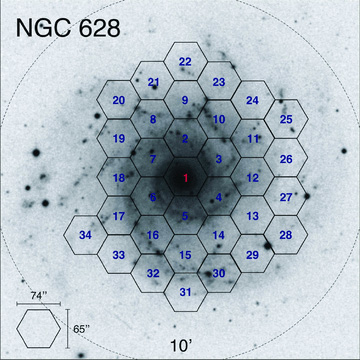
B-band Digital Sky Survey image of NGC 628. The mosaic of the PPAK pointings is shown as overlaid hexagons indicating the FOV of the central fibre bundle. The identification number of each pointing is indicated, as listed in Table 1. The circle indicates the D25 radius (in the B band). The image is 10 × 10 arcmin2 and it is displayed in top-north, left-east standard configuration.
Log of the observations.
| Date | Pointings |
| 06/10/28 | 1,2,3,9,10,22,23 |
| 07/12/10 | 1,4,5,6,7,8 |
| 07/12/11 | 14,15,16,17,18,19,30 |
| 07/12/12 | 11,12,13,25,29,31,32 |
| 08/08/09 | 11 |
| 08/10/30 | 24,26,27,28,29,33,34 |
| Date | Pointings |
| 06/10/28 | 1,2,3,9,10,22,23 |
| 07/12/10 | 1,4,5,6,7,8 |
| 07/12/11 | 14,15,16,17,18,19,30 |
| 07/12/12 | 11,12,13,25,29,31,32 |
| 08/08/09 | 11 |
| 08/10/30 | 24,26,27,28,29,33,34 |
4 DATA REDUCTION
Data reduction was performed using r3d (Sánchez 2006), in combination with iraf2 packages and e3d (Sánchez 2004). The reduction consists of the standard steps for fibre-based IFS. A master bias frame was created by averaging all the bias frames observed during the night and subtracted from the science frames. The different exposures taken at the same position on the sky were then combined, clipping the cosmic rays, using iraf routines. Then the locations of the spectra on the CCD were determined using a continuum illuminated exposure taken before the science exposures. Each spectrum was then extracted from the science frames. In order to reduce the effects of the cross-talk we did not perform a simple aperture extraction, which would consist of co-adding the flux within a certain number of pixels of location derived from the continuum illuminated exposure. Instead, we adopted a modified version of the Gaussian-suppression technique described in Sánchez (2006).
The new technique assumes a Gaussian profile for the projection of each fibre spectrum along the cross-dispersion axis. It basically performs a Gaussian fitting to each of the fibres after subtracting the contribution of the adjacent fibres in an iterative process. First, a simple aperture extraction is performed with a 5-pixel aperture. This initial guess of the flux corresponding to each spectrum is then used to model the profiles with a Gaussian function, adopting as centroid the location of the peak intensity determined from the continuum exposure. The width of the model Gaussian is taken from the average width of all the fibre profiles (σ∼2 pixels). In this first iteration, the aperture-extracted flux is used as the integrated flux of the Gaussian function. This modelled profile is then used, for each spectrum, to remove the contribution of the four adjacent fibre spectra. The resulting clean profile is then fitted with a Gaussian function, with the centroid and width parameters fixed, in order to derive a better estimation of the integrated flux. This new flux is used as the input for the next iteration of the process. It was found that with three iterations the procedure converges, increasing the signal-to-noise ratio (S/N) of the extracted spectra and reducing the effect of cross-talk.
The extracted flux, for each pixel in the dispersion direction, is stored in a row-stacked-spectrum (RSS) file (Sánchez 2004). Wavelength calibration was performed using HeHgCd lamp exposures obtained before and after each pointing, yielding an accuracy of rms ∼ 0.3 Å. Differences in the relative fibre-to-fibre transmission throughput were corrected by comparing the wavelength-calibrated RSS science frames with the corresponding frames derived from sky exposures taken during the twilight.
Although PPAK is equipped with fibres to sample the sky, in most of our pointings the sky fibres are located within an area containing significant signal from the galaxy. Accurate sky subtraction was therefore an important issue in the data reduction. For the different nights and pointings we adopted different sky-subtraction schemes depending on the position of the pointing. In some cases, a sufficient number of sky fibres are located in regions free from galaxy emission, and it was possible to perform an accurate sky subtraction of the individual pointings using these sky spectra. Once a certain frame is properly sky-subtracted, the sky spectrum of any adjacent frame, observed in the same night and under similar weather conditions, can be easily estimated. To do so the spectra of the 11 fibres in the sky-subtracted frame that overlap an adjacent frame (that has not been sky-subtracted) are combined. This combined spectrum is then subtracted from the corresponding combined spectrum of the 11 fibres of the adjacent frame. This produces an estimation of the sky spectrum in the adjacent frame that is then subtracted from all the spectra in that frame. Prior to this subtraction it is necessary to visually check that no residual of the galaxy is kept in the estimated sky spectrum, which can occur if the atmospheric transmission changed substantially between the observations of the two frames.
In other frames the sky observations taken during the night could be used to subtract the sky in the science observations, especially when the sky and target exposures are taken within a few minutes of each other. When the exposures were more widely separated in time it was necessary to combine different sky frames with different weights to derive good results. The criterion adopted to decide when a subtraction was good or not was to minimize the residuals in the typical emission features of the night spectrum. A thorough analysis of the sky subtraction and the residuals found in the reduction of this galaxy can be found in Paper I.
After reducing each individual pointing we built a single RSS file for the mosaic following an iterative procedure. The spectra of each pointing were scaled to those of the previous pointing by the average ratio in the 11 overlapping spectra. Those overlapping spectra were then replaced by the average between the previous pointing and the new rescaled spectra. The resulting spectra were incorporated into the final RSS file, updating the corresponding position table. By adopting this procedure the differences in the spectrophotometric calibration night-to-night and frame-to-frame are normalized to that of the first frame used in the process. For this reason, the mosaic was constructed starting from the central frame observed in the night of 2007 December 10, under nearly photometric conditions according to the Calar Alto extinction monitor. The final mosaic data set comprises 11 094 non-overlapping individual spectra, covering a FOV of ∼6 × 7 arcmin2, i.e. ∼70 per cent of the optical size of the galaxy (defined by D25 mag arcsec−2 radius in the B band), and therefore represents the largest spectroscopic survey of a single galaxy.
4.1 Accuracy of the flux calibration
Although particular care has been taken to achieve the best spectrophotometric calibration, there are many effects that can strongly affect it. Among them, the most obvious are the photon-noise from low surface brightness regions of the galaxy, the sky-background noise or variations in the weather conditions between the time when the spectrophotometric standards and the object were observed. This latter effect was reduced by the adopted mosaicking procedure in the data reduction, since the photometric calibration was renormalized to that of a particularly good night. Less obvious is the effect of inaccuracies in the sky subtraction. However, for low surface brightness regions this is one of the most important effects.
Since it is our goal to provide accurate spectrophotometric data, we performed a flux re-calibration on the data. To do so we used the flux-calibrated broad-band optical images from the SINGS legacy survey (Kennicutt et al. 2003). In particular, we compared our data set with the B, V, R and Hα images, since they are mostly covered by the wavelength range of our spectra. The photometric calibration of those images is claimed to be ∼5 per cent for the broad-band images and ∼10 per cent for the narrow-band images. They reach a depth of ∼25 mag arcsec−2 with a S/N of ∼10σ. Therefore, for the structures included in the FOV of our IFS data, the photometric errors of the imaging are dominated by the accuracy of the calibration, and not by the photon-noise.
The IFS mosaic was registered to the SINGS optical data by matching the coordinates of the galaxy bulge and foreground stars in the FOV (see the left-hand panel of Fig. 2). After this process the error in the astrometry of the IFS data was estimated to be ∼0.3 arcsec, based on the rms of the differences in the centroid of the stars and galaxy bulge. Once registered, the mosaic position table was used to extract aperture photometry from each broad-band image at the location of each fibre and with an aperture similar to that of the fibres. The photometry was transformed to flux (in cgs units) by using the counts-to-magnitude prescription in the SINGS documentation,3 and the zero-points included in Fukugita, Shimasaku & Ichikawa (1995). On the other hand, each spectrum in the mosaic was convolved with the corresponding transmission curve of the filters indicated before, in order to extract a similar flux fibre-to-fibre, based on the IFS data. This procedure provides us with 11 094 photometric points per band to compare between the two data sets.
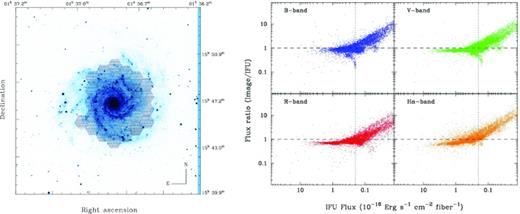
Left: SINGS B-band image of NGC 628 used to perform the absolute flux re-calibration. The position of each individual fibre of the IFS mosaic is shown overlaid to the real scale. Right: distribution of the ratio between the flux in the apertures corresponding to the PPAK fibres on each of the flux-calibrated broad-band images obtained from the SINGS ancillary data and the corresponding flux extracted from the IFU data. Each panel shows the results for the different imaging data: B-band (top-left panel), V-band (top-right panel), R-band (bottom left) and Hα (bottom-right panel). The horizontal dashed line indicates the one-to-one ratio, while the vertical dotted line indicates the adopted intensity cut for acceptable flux calibration.
The right-hand panel of Fig. 2 shows the ratio between the two sets of photometric points versus the flux extracted from the IFU data, for each of the considered filters. The figure shows the typical pattern obtained when comparing the flux ratio between two data sets with different depth, with the broad-band images clearly deeper than the spectroscopic data, as expected. Down to 0.2 × 10⁻¹⁶ erg s−1 cm−2 (∼5772 fibres) the ratio is ∼0.9 for all the fibres, with a standard deviation of ∼0.3 dex. Small differences in the transmission curves of the filters used in this calculation and the ones used by Fukugita et al. (1995) as well as the astrometric errors described before introduce uncertainties in the derived fluxes which increase the standard deviation. The uncertainties from the former source are difficult to estimate. However, the uncertainties introduced by astrometric errors are estimated to be at least ∼10 per cent by simulating different mosaic patterns, moving the location of fibres randomly within 0.3 arcsec (the uncertainty of our astrometry) and comparing the extracted photometry. Based on all these results we estimate our spectrophotometric accuracy to be better than ∼0.2 mag when we apply the re-calibration derived by this flux ratio analysis. The overall re-normalization factor applied to the IFS mosaic was 1.15, derived as the average of the ratios found on each band. This difference in the zero-point of the flux calibration lies within the expectations based on the estimated accuracy of our spectrophotometric calibration.
Fig. 3 shows in the left-hand panel, the comparison between the drift-scan spectrum of the central region of NGC 628 (blue line), published by Kennicutt et al. (2003) 4 and the integrated spectrum extracted from the spectrophotometrically re-calibrated PINGS mosaic (black line), after co-adding the spectra within a simulated aperture with the same size, location and PA as the SINGS drift scan. The SINGS drift scan corresponds to a 20 arcsec aperture and 70o PA. The right-hand panel of Fig. 3 shows a 100 Å width narrow-band map of the mosaic of NGC 628 centred at Hα, and the red box in the centre corresponds to the simulated aperture from which the IFS spectrum was extracted. The coordinates, size and PA of the aperture were obtained from the header of the SINGS data file. Some gaps in between the edges of the pointings are seen in this map; they are due to the re-centring of the individual pointings after comparing with the broad-band images as discussed above. As expected from the spectrophotometric re-calibration of the mosaic, there is a very good agreement between both data sets; both the general shape of the spectra and the strength of the spectral features match well. The left-hand panel of Fig. 3 shows in the lower part the relative difference between the two spectra, which is consistent with a null difference (in average) and within the error of the absolute flux calibration for most of the spectral range. As simulations with different position, apertures and mosaic versions showed, the small deviations in the continuum are due to the presence of a foreground star within the FOV of the simulated slit. The small disagreement at wavelengths shorter than 4000 Å is expected due to the degradation of the CCD sensitivity in the blue, as explained in detail in Paper I, where further comparisons with previous spectrophotometric data can be found. A slight mismatch of the wavelength resolution at the edges of the spectra is also noticed, being in the range of the expectations for such comparisons.

Left: comparison between the spectrum extracted for the central region of NGC 628 (shown in the right-hand panel) using the PPAK data (black line) after co-adding the spectra within a simulated aperture with the same size, location and PA as the SINGS legacy survey drift-scan (blue line, in the online version of the paper). The bottom panel shows the ratio between the two spectra. Right: narrow-band map of the PINGS mosaic of NGC 628 centred at Hα, the red box in the centre corresponds to the simulated aperture from which the IFS spectrum was extracted. Despite the different techniques used to derive both spectra, there is a clear agreement between them in most of the wavelength range.
Fig. 4 shows the comparison between two reconstructed V-band images of NGC 628. The image on the left was created after interpolating the aperture photometry extraction of the SINGS broad-band image. The image on the right was derived from the flux re-calibrated IFS data set, once each spectrum corresponding to a particular fibre was convolved with the filter response, as described before. In order to create a regularly gridded image, the data were interpolated using e3d (Sánchez 2004), adopting a natural-neighbour non-linear interpolation scheme, and a final pixel scale of 1 arcsec pixel−1. The areas not fulfilling our criteria for accurate spectrophotometry (FV < 0.210−16 erg s−1 cm−2) were masked.
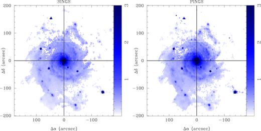
Reconstructed V-band images of NGC 628. Left: image created after interpolating the aperture photometry extraction of the SINGS broad-band image. Right: interpolated image derived after multiplying each spectrum of the IFS mosaic with the filter response curve. Both images were created with a regular grid of 1 arcsec pixel−1. The areas not satisfying our criteria of accurate spectrophotometry were masked. The perpendicular lines are centred at the mosaic's reference point. Offsets are in arcsec.
5 ANALYSIS AND RESULTS
In order to extract physical properties of the galaxy from the data set it is necessary to perform different kinds of analyses. In particular, for each spectrum we need to identify the emission lines of ionized gas, and decouple this emission from the underlying stellar population. Particular care has to be taken in this decoupling technique, since some of the emission lines (e.g. Hβ) may be strongly affected by underlying absorption features.
The decoupling of the stellar population from the emission lines was performed adopting a scheme summarized here: (i) a set of detected emission lines was identified in the integrated spectra of the stronger H ii regions in the outer part of the galaxy. (ii) For each spectrum in the data set, the underlying stellar population was fitted by a linear combination of a grid of single-stellar population (SSP) templates, after correcting for the appropriate systemic velocity and velocity dispersion (including the instrumental dispersion which dominates the total observed dispersion), and taking into account the effects of dust attenuation. A spectral region of 30 Å width around each detected emission line was masked prior to the linear fitting, including also the regions around the sky lines (Sánchez et al. 2007a). (iii) Once we derived a first approximation of the spectrum of the underlying stellar population, this was subtracted from the original spectrum to obtain a pure emission-line spectrum. (iv) To derive the intensity of each detected emission line, each of these clean spectra in the data set was fitted to a single Gaussian function per emission line plus a low-order polynomial function. Instead of fitting emission lines over the entire wavelength range simultaneously, for each spectrum we extracted shorter wavelength ranges that sampled one or a few of the analysed emission lines, in order to characterize the residual continuum with a simple polynomial function, and to simplify the fitting procedure. When more than one emission line was fitted simultaneously, their systemic velocities and FWHMs were forced to be equal (since the FWHM is dominated by the instrument resolution), in order to decrease the number of free parameters and increase the accuracy of the deblending process (when required). (v) Finally, for each spectrum in the data set a pure gas-emission spectrum was created, based on the results of the last fitting procedure, using only the combination of Gaussian functions. This model was then subtracted from the original data, spectrum by spectrum, to produce a data set of gas-free spectra. These spectra are then fitted again by a combination of SSP, as described before (but without masking the spectral range around the emission lines, in this case), deriving the luminosity-weighted age, metallicity and dust content of the composite stellar population. Appendix A gives a detailed description of the fitting procedure, indicating the basic algorithms adopted, and including estimates of the accuracy of the SSP-based modelling and the derived parameters based on simulations. The 2D maps of the emission-line intensities and physical properties shown in the following sections were constructed based on the pure gas-emission mosaics described above.
5.1 Integrated spectrum
A particularly interesting use of IFS data sets is the combination of the observed spectra to produce an integrated spectrum of the object, using the IFU as large aperture spectrograph. This high S/N integrated spectrum can be used to derive, for the first time, the real average spectroscopic properties of the galaxy, as opposed to previous studies that attempted to describe its average properties by the analysis of individual spectra taken at different regions. The most similar approach would be the spectrum derived by using a drift-scanning technique [e.g. Moustakas & Kennicutt (2006b) and part of the ancillary data of the SINGS survey], although in those studies (especially for the latter) the fraction of galaxy covered by the spectra was much less than for the spectrum presented here. Another advantage of the use of an IFU with respect to the drift-scan technique is that the former allows a comparison between the integrated and the spatially resolved properties of the galaxy.
A good amount of the fibres in the IFS mosaic of NGC 628 do not contain enough S/N or do not contain signal at all (i.e. spectra with a flat continuum consistent with zero-flux), as the fibres were sampling regions where the intrinsic flux from the galaxy is low or null (e.g. borders of the mosaic, intra-arms regions, etc.). In order to get rid of spectra where no information could be derived, we obtained a clean version of the IFS mosaic of NGC 628 by applying a flux threshold cut choosing only those fibres with an average flux along the whole spectral range greater than 10−16 erg s−1 cm−2 Å−1. Furthermore, bad fibres (due to cosmic rays and CCD cosmetic defects) and foreground stars (10 within the observed FOV of NGC 628) were removed from the mosaic. This procedure resulted in a refined mosaic version which includes only those regions with high-quality spectrophotometric calibration. The total number of spectra in the clean IFS mosaic version of NGC 628 is 6949. The top panel of Fig. 5 shows the integrated spectrum of NGC 628 derived by co-adding the spectra within the clean IFS mosaic version of the galaxy.
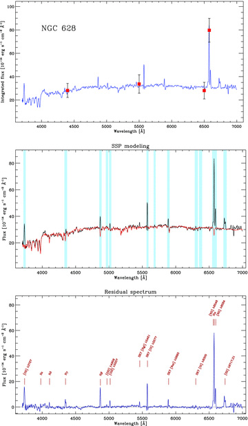
Integrated spectrum of NGC 628. The red solid squares in the top panel indicate the integrated flux derived from the B, V, R and Hα images. The middle panel shows the SSP model fitting (red line, in the online version) to the spectrum, the light-blue bands correspond to the spectral regions masked during the fitting. The bottom panel shows the residual after subtracting the model from the original spectrum; the detected emission lines have been labelled.
The integrated spectrum of NGC 628 shows a characteristic stellar continuum with absorption features and emission lines superimposed. Hα, Hβ, [O ii]λ3727, [O iii]λ5007, the [N ii]λ λ6548,84 and λ λ6717,31 doublets are clearly identified. Less obvious are the Hγ and [O iii]λ4959 lines. Sky residuals are also present in the spectrum, especially the [O i]λ5577 and [Na i]λ5893 lines. The red solid squares (in the online version) correspond to the integrated flux derived from the B, V, R and Hα images of the SINGS ancillary data, obtained during the spectrophotometric re-calibration, using the same apertures of the IFU data and co-adding them in a similar way as the integrated spectrum. The position of these data-points with respect to the continuum (in the case of the broad-band images) and the peak of the Hα line in the spectrum corroborates the accuracy of the absolute flux calibration. The co-added region comprises ∼90 per cent of the total flux of the galaxy in V band, as estimated from corresponding SINGS image. An analysis similar to that described above was performed on this integrated spectrum to derive the main physical properties of both the ionized gas and the stellar population.
5.1.1 Integrated stellar populations
The middle panel of Fig. 5 shows the best SSP model fit to the integrated spectrum superimposed in red colour. The light-blue bands correspond to the spectral regions masked during the fitting as explained above. They coincide with the position of the strongest redshifted emission lines and regions of bright sky residuals. Note the strength of the underlying stellar absorptions in the Balmer lines. The multi-component SSP model accurately matches the continuum of the integrated spectrum, within an error of the ∼3 per cent. Most of the discrepancies are in regions clearly dominated by imperfections in the sky subtraction, due to the strength of the night sky lines [e.g. at ∼ λ5577; see Sánchez et al. (2007a) and Paper I]. In order to evaluate the possible effects of these residuals in the derivation of the main properties of the stellar population the analysis was repeated for the wavelength range between λ4100 and λ5400 Å, where there are no such strong atmospheric features. For this wavelength range, the model matches the continuum within a ∼2 per cent. In the UV regime the errors are sometimes larger than this value.
Table 2 lists the luminosity-weighted age, metallicity and dust attenuation of the best-fitting model for the two cases considered here: one using the entire spectral range in the fitting process and the other using the reduced range described before. There is a very good agreement between the results derived in both cases. Based on the results from the simulations (see Appendix), we expect an error of 10-20 per cent in the derivation of the age, and of a ∼5 per cent in the derivation of the metallicity. These errors do not take into account the systematics, due to the applied algorithm, the current code and the templates adopted, or the known degeneracies in the derivation of the age and the metallicity, and therefore the expected discrepancies with previous published results are much larger than the ones estimated on the basis of the simulations. From these fits we may conclude that the average stellar population of NGC 628 is dominated by an old component of ∼9 Gyr, but with a subsolar metallicity ([Z/H]∼−0.45). Although synthesis modelling is nowadays widely used, we have to take into account the age–metallicity degeneracy problem that plagues most spectral fitting techniques. The most frequently used technique to derive the age and metallicity of the stellar population in galaxies is to measure certain line strength indices, such as the Lick/IDS index system (e.g. Burstein et al. 1984; Faber et al. 1985; Burstein, Faber & Gonzalez 1986; Gorgas et al. 1993; Worthey 1994). For this purpose, one generally tries to use a combination of indices that are most orthogonal in the parameter space (i.e. age and metallicity). In order to cross-check the results based on the fitting procedure, we measured the equivalent width of Hβ (primarily sensitive to the age) and Mgb (primarily sensitive to the metallicity), of the integrated spectrum.
Properties of the average stellar population.
| Analysis method | Age (Gyr) | Metallicity | A (mag) (mag) | |
| (Z) | [Z/H] | |||
| SSP fit, 3700–6800 Å | 8.95 | 0.007 | −0.44 | 0.4 |
| SSP fit, 4100–5400 Å | 8.40 | 0.007 | −0.44 | 0.8 |
| Hβ versus Mgb indices | 9.78 | 0.008 | −0.42 | − |
| Analysis method | Age (Gyr) | Metallicity | A (mag) | |
| (Z) | [Z/H] | |||
| SSP fit, 3700–6800 Å | 8.95 | 0.007 | −0.44 | 0.4 |
| SSP fit, 4100–5400 Å | 8.40 | 0.007 | −0.44 | 0.8 |
| Hβ versus Mgb indices | 9.78 | 0.008 | −0.42 | − |
aDust continuum attenuation.
Properties of the average stellar population.
| Analysis method | Age (Gyr) | Metallicity | A (mag) | |
| (Z) | [Z/H] | |||
| SSP fit, 3700–6800 Å | 8.95 | 0.007 | −0.44 | 0.4 |
| SSP fit, 4100–5400 Å | 8.40 | 0.007 | −0.44 | 0.8 |
| Hβ versus Mgb indices | 9.78 | 0.008 | −0.42 | − |
| Analysis method | Age (Gyr) | Metallicity | A (mag) | |
| (Z) | [Z/H] | |||
| SSP fit, 3700–6800 Å | 8.95 | 0.007 | −0.44 | 0.4 |
| SSP fit, 4100–5400 Å | 8.40 | 0.007 | −0.44 | 0.8 |
| Hβ versus Mgb indices | 9.78 | 0.008 | −0.42 | − |
aDust continuum attenuation.
The equivalent widths of the absorption lines were derived using the bandpass definitions from the Lick index system revised by Trager et al. (1998), shifted to the redshift of the object, as described in Sánchez et al. (2007c). To derive the age and metallicity from the measured indices, we have adopted the model grid from Thomas, Maraston & Bender (2003), implemented in the rmodel code.5 The resulting estimates of the age and metallicity, based on the absorption line index analysis, are listed in Table 2. Despite the strong conceptual differences between these methods and the fitting technique described before, the results are very consistent with the values obtained in both the full and reduced wavelength range SSP fitting.
5.1.2 Integrated properties of the ionized gas
The bottom panel of Fig. 5 shows the pure emission-line spectrum of NGC 628 obtained after subtracting the underlying stellar population from the integrated spectrum. As expected, the spectrum is dominated by a set of emission lines, plus a residual continuum consistent with a zero average intensity. This procedure reveals additional emission lines, like Hδ and Hε. All the detected lines have been labelled with their standard notation. Each of these emission lines was fitted with a single Gaussian function, as described before, in order to derive their strengths. Fig. 6 shows an example of the fits in the wavelength range between 6500 and 6800 Å. The black solid line corresponds to the pure emission-line spectrum of NGC 628, the red dashed line shows the best fitted model, consisting of six Gaussian functions, assuming a single Gaussian fit to each of the emission lines detected in this wavelength range: the [N ii] doublet, Hα, He iλ6678 (very faint) and the [S ii] doublet. In this particular case both the systemic velocity and velocity dispersion were forced to be the same for all the emission lines, in order to increase the accuracy of the derived parameters. The ratio between the two [N ii] lines included in the spectral range was fixed to the theoretical value (Osterbrock & Ferland 2006). A similar procedure was applied to the rest of the emission lines. By adopting this procedure, it is possible to accurately deblend the different emission lines.
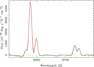
Example of the fitting procedure applied to derive the intensity flux of the detected emission lines. The black solid line corresponds to the pure emission-line spectrum of NGC 628, covering the wavelength range between 6500 and 6800 Å. The red dashed line shows the best-fitting model describing the emission lines, which comprises a single Gaussian function for each of them. The green dotted line shows the residual spectrum, once the previous model has been subtracted.
Table 3 lists the emission-line intensities derived using this procedure, including for each of the detected emission lines its standard identification, the laboratory rest-frame wavelength and the estimated intensity normalized to the observed flux of Hβ in units of 10−15 erg s−1 cm−2. They are shown in the columns labelled as F(λ)/Hβ. The observed [O iii] ratio shown in Table 3 is consistent with the well-known theoretical value between these lines (Storey & Zeippen 2000). The associated 1σ errors are solely due to the statistical uncertainty σstat in the measurement of the flux intensity. Thereafter, the observed line intensities were corrected for reddening using the Balmer decrement according to the reddening function of Cardelli, Clayton & Mathis (1989), assuming R≡AV/E(B−V) = 3.1. Theoretical values for the intrinsic Balmer line ratios were taken from Osterbrock & Ferland (2006), assuming case B recombination (optically thick in all the Lyman lines), an electron density of ne = 100 cm−3 and an electron temperature Te = 104 K. The last column of Table 3 shows the reddening-corrected emission line fluxes for the integrated spectrum, designated by I(λ)/Hβ. These flux ratios can be used to derive the average properties of the ionized gas in the galaxy. The adopted reddening curve normalized to Hβ, f(λ), is shown in the second column of the table. Although higher-order Balmer lines were detected in the integrated spectrum, no Balmer lines beyond Hγ were used for the determination of c(Hβ), as the associated error of the measurement of these lines in the residual spectrum yielded high uncertainties in the computed c(Hβ), due to their low S/N; therefore the c(Hβ) value was derived using the Hα/Hβ ratio solely. No auroral lines were detected either in the integrated or residual spectrum. The low strength of the [O iii] lines suggests a relatively high metallicity for the integrated abundance of NGC 628, as it will be shown hereafter.
Integrated line intensities for NGC 628. The first column corresponds to the Emission-line identification, with the rest-frame wavelength, the second one corresponds to the adopted reddening curve normalized to Hβ. The F(λ)/Hβ column corresponds to the observed flux, while the I(λ)/Hβ to the reddening corrected values; normalized to Hβ. The values in parentheses correspond to the 1σ errors calculated as explained in the text. The observed flux in Hβ is in units of 10−15 erg s−1 cm−2. The last row shows the number of fibres from which the integrated spectra were extracted.
| Line | f(λ) | F(λ)/Hβ | I(λ)/Hβ |
| [O ii]λ3727 | 0.32 | 1.494 (0.046) | 2.138 (0.320) |
| H 8 + He iλ3889 | 0.29 | 0.158 (0.032) | 0.217 (0.054) |
| Hδλ4101 | 0.23 | 0.165 (0.032) | 0.214 (0.051) |
| Hγλ4340 | 0.16 | 0.511 (0.023) | 0.609 (0.083) |
| Hβλ4861 | 0.00 | 1.000 (0.014) | 1.000 (0.052) |
| [O iii]λ4959 | −0.03 | 0.111 (0.010) | 0.108 (0.017) |
| [O iii]λ5007 | −0.04 | 0.329 (0.010) | 0.315 (0.040) |
| He iλ5876 | −0.20 | 0.299 (0.012) | 0.239 (0.031) |
| [N ii]λ6548 | −0.30 | 0.383 (0.013) | 0.276 (0.035) |
| Hαλ6563 | −0.30 | 3.998 (0.041) | 2.870 (0.352) |
| [N ii]λ6584 | −0.30 | 1.111 (0.016) | 0.795 (0.098) |
| [S ii]λ6717 | −0.32 | 0.619 (0.011) | 0.435 (0.054) |
| [S ii]λ6731 | −0.32 | 0.393 (0.010) | 0.276 (0.035) |
| [O iii]λ5007/λ4959 | 2.96 (0.28) | 2.92 (0.58) | |
| [S ii]λ6717/λ6731 | 1.57 (0.14) | 1.58 (0.28) | |
| F(Hβ) λ4861 | 1549.4 | ||
| c(Hβ) | 0.48 (0.05) | ||
| AV | 1.04 | ||
| Extraction fibres | 6949 |
Although particular care has been taken in the flux calibration of the spectra within the mosaic, the absolute flux intensity listed in Table 3 has to be treated with caution. On one hand, not all of the galaxy surface has been covered by our IFS observations, as can be seen in Fig. 1. In particular some of the brighter H ii regions, located to the east of NGC 628, are not included in the FOV of our mosaic. This causes to underestimate the intensity of all the lines. By a rough estimation, based on the D25 optical radius (B band), we consider that our IFS mosaic covers ∼70 per cent of the galaxy size. On the other hand, the central fibre bundle of PPAK has a filling factor of ∼65 per cent, as mentioned in Section 3, which leads to a corresponding underestimation of the integrated flux. In the particular case of this mosaic, a dithering scheme necessary to compensate for this incomplete sampling was adopted only for the central pointing, where the emission lines are in general weak. All together, we consider that it is necessary to apply a correction of a factor of ∼2.2 to take into account the aperture and sampling effects described before. As mentioned before, NGC 628 has been extensively studied before in several publications. In particular, different authors have reported on the Hα intensity flux, using different procedures, from photoelectric photometers to narrow-band imaging. Table 4 lists a summary of these published values, together with the value derived from our integrated spectrum and considering the flux correction factor described above. Despite the different biases introduced by the different methods, there is substantial agreement between the previously published results and our reported value for the integrated Hα flux of the galaxy.
Comparison between different Hα fluxes reported for NGC 628 in the literature. Fluxes in units of 10−11 erg s−1 cm−2.
| Flux | Reference |
| 1.07 | Kennicutt (1983) |
| 0.87 | Young et al. (1996) |
| 1.51 | Hoopes et al. (2001) |
| 1.05 | Marcum et al. (2001) |
| 1.02 | Kennicutt et al. (2008) |
| 1.14 | Current study |
| Flux | Reference |
| 1.07 | Kennicutt (1983) |
| 0.87 | Young et al. (1996) |
| 1.51 | Hoopes et al. (2001) |
| 1.05 | Marcum et al. (2001) |
| 1.02 | Kennicutt et al. (2008) |
| 1.14 | Current study |
The derived dust extinction, AV = 1.04, is larger than the one derived from the analysis of the stellar populations (AV∼ 0.4 mag). This result is not surprising, since both methods sample different regions of the galaxy. While the underlying continuum is dominated by the stellar components of the central regions, clearly brighter, the ionized gas spectrum is dominated by the star-forming regions in the spiral arms. These latter regions are known to be more attenuated by dust, due to the star-forming process (e.g. Calzetti 2001). Indeed, the extinction law derived by Calzetti (1997) for star-forming galaxies shows that the typical extinction in the emission lines of these objects is approximately double that in their stellar continuum.
The integrated flux of Hα and [O ii]λ3727 can be used to determine a rough value of the global SFR in this galaxy. The intensities of both lines were corrected by dust extinction, adopting the AV value and the aperture correction mentioned before. Absolute luminosities were derived by assuming a standard ΛCDM cosmology with H0 = 70.4, Ωm = 0.268 and ΩΛ = 0.73, and a luminosity distance of 9.3 Mpc (Hendry et al. 2005). The derived luminosities are LHα∼ 3.08 and L[O ii]∼ 2.30, in units of 1041 erg s−1. The values of the SFR were derived adopting the classical relations by Kennicutt (1998), obtaining SFR ∼2.4 and 3.2 M⊙ yr−1, based on the Hα and [O ii] luminosities, respectively.
Different possible mechanisms can be responsible for the ionization in emission-line galaxies. The nature of the ionization can be derived from ratios of the usual diagnostic lines (Baldwin, Phillips & Terlevich 1981, hereafter BPT; Veilleux & Osterbrock 1987). Based on the values listed in Table 3, it was found that log10([N ii]λ6584/Hα) ∼ −0.56 and log10([O iii]λ5007/Hβ) ∼ −0.5. These line ratios correspond to the expected values for star-forming galaxies and/or H ii regions (e.g. Sánchez et al. 2005, 2007c), far away from any of the boundary regions in the [O iii]/Hβ versus [N ii]/Hα diagnostic diagram. Therefore, it is clear that the dominant ionization mechanism in the integrated spectrum of NGC 628 is due to hot OB stars (H ii regions), as expected, since no previous study has reported any kind of nuclear activity in this galaxy.
The (volume-averaged) ionization parameter, defined as the ratio of the density of ionizing photons to the particle density:  , where
  is the flux of ionizing photons produced by the exciting stars above the Lyman limit, Rs the radius of the Strömgren sphere, n the number density of hydrogen atoms and c the speed of light. This parameter determines the degree of ionization at any particular location within the nebula. As discussed in the next section, many of the empirical methods commonly used to derive the chemical abundance of a star-forming region are sensitive to this parameter, and for some ranges of metallicity, they are not useful unless the ionization parameter can be constrained within a small range of possible values.
5.1.3 Integrated oxygen abundance
Galaxies in the local universe have been used as an anchor point to determine the evolution of the metallicity (based on the gas-phase oxygen abundance), along different cosmological periods. The global metallicity of a given galaxy is represented by its oxygen abundance. The rest of the elements vary within the same fractions as those found in the Sun. However, while the determination of this observable at high redshift normally describes the average value of the galaxies as a whole (due to aperture effects), in the local universe most of these determinations are based on studies of a number of discrete H ii regions. The integrated spectrum of NGC 628 can be used to perform an integrated abundance analysis in a consistent way as the studies performed over high-redshift galaxies, with the advantage that the results of the integrated study can be compared with the abundances of resolved regions within the galaxy. In this section, we present a chemical abundance analysis of the integrated spectrum of NGC 628 based on a suite of different empirical abundance diagnostic methods. A more detailed comparison between the integrated and spatially resolved abundances will be presented in a subsequent paper (Rosales-Ortega et al., in preparation).
Given the limitations imposed by the non-detection of auroral temperature-sensitive emission lines (such as [O iii]λ4363 or [N ii]λ5755) in H ii regions of low-excitation and/or low surface brightness, empirical methods based on the use of strong, easily observable optical lines have been developed throughout the years. Although abundances derived in this way are recognized to suffer considerable uncertainties, they are believed to be able to trace large-scale trends in galaxies. Following these ideas, several abundance calibrators have been proposed involving different emission-line ratios and have been applied to determine oxygen abundances in objects as different as individual H ii regions in spiral galaxies, dwarf irregular galaxies, nuclear starburst and the integrated abundances of spiral galaxies (e.g. Kobulnicky, Kennicutt & Pizagno 1999; Pilyugin, Contini & Vílchez 2004, and references therein).
In order to derive the characteristic chemical abundance of NGC 628, a set of empirical calibrators was applied to the integrated spectrum. Different abundance estimators were chosen in order to explore the effect of a particular calibration depending on the physical properties of the galaxy. By far, the most commonly used such ratio is ([O ii]λ3727 +[O iii]λ4959, λ5007)/Hβ, known as the R23 method (Pagel et al. 1979). The logic for the use of this ratio is that it is not affected by differences in relative elemental abundances, and remains essentially constant within a given giant H ii region despite variations in excitation (Diaz et al. 1987). However, there is an ambiguity inherent to this method since there are two values of abundance corresponding to a given value of R23, i.e. the lower branch increases with increasing abundance, while the upper branch shows an opposite behaviour, i.e. R23 decreases with increasing abundance. Another drawback of using R23 (and many of the other emission-line abundance diagnostics) is that it depends also on the ionization parameter. From this category, two methods were applied: the McGaugh (1991) (hereafter M91) and the Kobulnicky & Kewley 2004 (hereafter KK04) calibrations, which are theoretical methods based on photoionization models. Both take into account the ionization parameter to produce an estimate of the metallicity. The estimated accuracy of these methods is ∼ ±0.15 dex.
In order to discriminate between the different R23 branches, we used the [N ii]λ6584/[O ii]λ3727 ratio following the prescriptions by Kewley & Dopita (2002). The [N ii]/[O ii] ratio is not sensitive to the ionization parameter to within ±0.05 dex, and it is a strong function of metallicity above log([N ii]/[O ii]) ≳–1.2, where the division between the upper and lower branches occurs. The log([N ii]/[O ii]) value for the integrated spectrum of NGC 628 is −0.43, i.e. indicating that the R23 value of the integrated spectrum for NGC 628 (log R23 = 0.41) corresponds to the upper branch of the R23 relation.
Another subset of estimators was chosen from the category of empirical strong-line methods; they correspond to the N2 calibration (first proposed by Storchi-Bergmann, Calzetti & Kinney 1994, but using the definition after Denicoló, Terlevich & Terlevich 2002), and the O3N2 calibration [first proposed by Alloin et al. (1979), but using the definition by Pettini & Pagel (2004)]. These two indices have the virtue of being single-valued; however, they are affected by the low-excitation line [N ii]λ6584, which may arise not only in bona fide H ii regions, but also in the diffuse ionized medium, which is an issue for spectra integrated within extended regions, such as the integrated spectrum of NGC 628. The estimated uncertainty of the derived metallicities is ∼ ±0.2 dex.
The Pilyugin & Thuan 2005 (hereafter PT05) calibration is based on an updated version of the Pilyugin (2001) estimator, obtained by empirical fits to the relationship between R23 and Te metallicities for a sample of H ii regions. This estimator was also considered to determine the integrated abundance of NGC 628. This calibration includes an excitation parameter P that takes into account the effect of the ionization parameter. The PT05 calibration has two parametrizations corresponding to the lower and upper branches of R23. As in the case of the M91 and KK04 calibrators, the [N ii]/[O ii] ratio was used to discriminate between the two branches of the R23 relation.
The last strong-line empirical method considered is a combination of the flux–flux (or ff-relation) found by Pilyugin (2005) and parametrized by Pilyugin, Thuan & Vílchez (2006), the t2−t3 relation between the O+ and O++ zones electron temperatures for high-metallicity regions proposed by Pilyugin (2007) and an updated version of the Te-based method for metallicity determination (Izotov et al. 2006). According to these authors, the combination of these methods solves the problem of the determination of the electron temperatures in high-metallicity H ii regions, where faint auroral lines are not detected. However, the abundances determined through this method rely on the validity of the classic Te method, which has been questioned for the high-metallicity regime in a number of studies by comparisons with H ii region photoionization models (Stasińska 2005). The abundances derived through this method will be referred as (O/H)ff or ff–Te abundances.
The advantages and drawbacks of all these different calibrators have been thoroughly discussed in the literature (e.g. Pagel, Edmunds & Smith 1980; Kennicutt & Garnett 1996; Kewley & Dopita 2002; Pérez-Montero & Díaz 2005; Kewley & Ellison 2008). Regrettably, comparisons among the metallicities estimated using these methods reveal large discrepancies. They are usually manifested as systematic offsets in metallicity estimates, with high values corresponding to theoretical calibrations and lower metallicities estimated by electron temperature metallicities, with offsets as large as 0.5 dex in log(O/H) units (Liang et al. 2006).
The calculated oxygen abundances [in units of 12 + log(O/H)] derived for each of the calibrators listed above are shown in Table 5. The uncertainties correspond to the 1σ error found by propagating the errors through a Monte Carlo simulation by using Gaussian distributions with a width equal to the errors of the emission-line intensities, modulated by recomputing the distribution 500 times. These abundances are plotted in Fig. 7. The red solid points (in the online version) correspond to the R23 methods, the green points to the index-empirical methods and the blue points to the different methods proposed by Pilyugin and collaborators. The red-open circles correspond to an arbitrary −0.5 dex offset of the R23 methods (these offsets are included given the well-known systematic offset of the R23 theoretical-based calibrations). The horizontal dotted line corresponds to the oxygen solar abundance 12 + log(O/H) = 8.7 (Scott et al. 2009).
Integrated oxygen abundances for NGC 628 in units of 12+log(O/H). The column designations correspond to the following abundance calibrators: M91, McGaugh (1991); KK04, Kobulnicky & Kewley (2004); N2, Denicoló et al. (2002); O3N2, Pettini & Pagel (2004); PT05, Pilyugin & Thuan (2005); (O/H)ff, ff–Te method (as explained in the text).
| log R23 | M91 | KK04 | N2 | O3N2 | PT05 | (O/H)ff |
| 0.41 | 8.90 ± 0.14 | 9.06 ± 0.11 | 8.62 ± 0.16 | 8.71 ± 0.11 | 8.32 ± 0.15 | 8.55 ± 0.09 |
| log R23 | M91 | KK04 | N2 | O3N2 | PT05 | (O/H)ff |
| 0.41 | 8.90 ± 0.14 | 9.06 ± 0.11 | 8.62 ± 0.16 | 8.71 ± 0.11 | 8.32 ± 0.15 | 8.55 ± 0.09 |
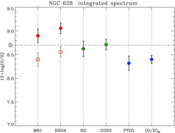
Comparison of the integrated oxygen abundance of NGC 628 derived for different estimators. Red solid points correspond to R23 calibrators, green points to index-empirical methods and blue points to the different methods proposed by Pilyugin and collaborators. The open circles correspond to an arbitrary −0.5 dex offset of the R23-based methods. The horizontal dashed line corresponds to the oxygen solar value.
The two R23 methods derive super-solar metallicity values, while the PT05 oxygen value corresponds to the lowest metallicity obtained. The index-empirical methods, N2 and O3N2, stand in between the metallicities derived through the R23 and the PT05 + ff–Te methods. Interestingly, the R23 calibration metallicities which were shifted to a lower value (red-open circles) are in close agreement (within the errors) to the pure-empirical and the ff–Te based metallicities. The mean oxygen abundance derived from all the methods is 12 + log(O/H) =8.69 ± 0.31.
Previous studies have determined the oxygen abundance in this galaxy based on spectroscopic imaging spectrophotometry observations of different H ii regions. In particular, McCall et al. (1985) analysed a sample of H ii regions within a radius of ∼200 arcsec, basically coincident with the area sampled by our IFS survey. They reported a range of oxygen abundances between 12 + log(O/H) ∼8.7–9.3 (by employing a method based on the R23 index), with a considerable decline from the inner to the outer parts. Belley & Roy (1992) obtained reddenings, Hβ equivalent widths, diagnostic line ratios and metallicities for 130 H ii regions by the implementation of imaging spectrophotometry. They derived an abundance gradient of NGC 628 based on the [O iii]/Hβ empirical calibrator (Edmunds & Pagel 1984). Their values range between 12 + log(O/H) ∼ 8.4 and 9.2, covering a large baseline in galactocentric distances (up to ρ∼ 2ρeff). Although this was not a strict spectroscopic study, given the number of H ii regions analysed, the work of Belley & Roy (1992) stood up to now as the most complete 2D description of the emission-line chemistry of NGC 628. Subsequently, van Zee et al. (1998) reported the oxygen abundances of the H ii regions in an outer ring between ∼150 and ∼300 arcsec radius. They found that the decline in the abundance continues, and the oxygen abundance ranges between 12 + log(O/H) ∼ 8.10 and 8.95 (using a modified version of the M91 calibrator). More recently, Castellanos et al. (2002b) observed a reduced set of H ii regions in the optical and near-infrared where they were able to measure temperature-sensitive emission lines. They reported an average oxygen abundance of 12 + log(O/H) ∼ 8.23. However these H ii regions are located beyond the FOV of our IFS mosaic, at galactocentric distances where, given the well-known radial metallicity gradient of this galaxy (Ferguson et al. 1998), the oxygen abundance is expected to be lower than the integrated metallicity derived at inner radii. Therefore, we cannot compare the integrated O/H abundance derived in this work with the values of Castellanos et al. (2002b) due to the non-coincident geometry. On the other hand, the range of oxygen abundances reported by the previous spectroscopic and imaging spectrophotometry studies agree perfectly with the integrated abundances derived through the R23 methods and with the mean-integrated abundance of NGC 628.
The integrated properties of the ionized gas derived in this chapter need to be compared with the resolved properties in order to analyse the validity of the results obtained from the integrated analysis, taking into account different effects, such as the extinction or the contribution of the diffuse interstellar emission. These points will be addressed in the following sections.
5.2 Spatially resolved properties of the galaxy
In this section we present the results obtained by applying the spectra fitting technique described in Section 5 to each individual spectrum of the data set. As indicated in Appendix A, the technique allows the decoupling of the spectral energy distribution (SED) of the underlying stellar population from that of the ionized gas. This step is needed to derive the intensities of the different emission lines detected in each spectrum accurately. In addition, when the S/N is high enough this fitting technique can be used to derive the physical parameters that characterize the composite stellar population: the luminosity-weighted age, metallicity and dust attenuation.
5.2.1 Distribution of the stellar populations
As shown in Appendix A, the results from simulations indicate that an individual spectrum does not have, in general, the required S/N to derive accurate values of the physical parameters that characterize the composite stellar population. However, the average spectra in concentric annuli do possess the required S/N, up to ∼120 arcsec (∼0.4ρ25 or ∼5.4 Kpc) in linear-projected galactocentric radii.
In order to study the distribution of the properties of the stellar population we obtained azimuthally averaged spectra by co-adding all the spectra in the mosaic within successive rings of 5 arcsec, starting from the central emission peak of the galaxy. These azimuthally averaged spectra were then analysed using the fitting procedure described above. Fig. 8 shows the radial distributions of the luminosity-weighted ages (left-hand panel) and metallicities (right-hand panel), derived by this method. The adopted error bars correspond to the typical errors estimated from the simulations (Appendix A) for a S/N of ∼100.
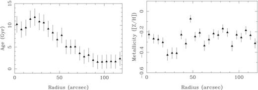
Left-hand panel: radial distribution of the luminosity-weighted age (in Gyr) of the stellar population based on the fitting procedure using the combination of multiple SSPs. Right-hand panel: similar distribution for the luminosity-weighted metallicity, relative to the solar one (Z/H).
It is important to stress here that the accuracy of the absolute scale of the ages is not as good as the relative one, since the former is much more model dependent than the second. The age distribution shows, in general, a gradient, with older stellar populations at the central regions of the galaxy and younger ones at the outer regions. However, the oldest stellar populations are not found in the centre of the galaxy, but in a circumnuclear ring at ∼25 arcsec radius, with an inversion of the gradient at smaller radii. This region corresponds to the central kpc of the galaxy. At larger radii, the stellar population becomes steadily younger, at a rate of ∼0.20 Gyr kpc−1, up to a radius of ∼100 arcsec (∼4.5 kpc), and then becomes stable with an age of ∼1 Gyr, on average. On the other hand, the radial distribution of the metallicity of the stellar populations does not show such a clear trend, remaining nearly constant at any radii with a larger dispersion in the values. Both distributions show a similar shape than the one presented by MacArthur, González & Courteau (2009), using a similar technique over classical slit-spectroscopy data, although their data show a larger dispersion.
The luminosity-weighted age and metallicity, derived from the plotted values, are ∼8.2 Gyr and Z∼ 0.01 ([Z/H]∼ −0.27), consistent with the values derived from the integrated spectrum (Table 2).
The gradient found in the stellar population of NGC 628 (with the older stellar populations in the centre) is common in late-type galaxies. Gadotti & dos Anjos (2001) found that ∼60 per cent of this kind of galaxies show a negative colour gradient in the U−B and B−V colours that it is most likely due to a gradient in the age of the stellar populations, with the younger populations in the outer regions. Differences between the colours in the central bulges (redder) and the outer discs (bluer) are also reported in other studies (e.g. Peletier & Balcells 1996). NGC 628 was included in the sample studied by Gadotti & dos Anjos (2001), and they reported a negative colour gradient in this galaxy up to a radius of ∼5 arcmin, qualitatively in agreement with the trend found here based on the analysis of our IFS data set.
As mentioned before, Ganda et al. (2007) presented a study based on the IFS observation of the central core of NGC 628, using SAURON. The total FOV of their observation was 33 × 41 arcsec2, with a spatial sampling of ∼1 arcsec. This FOV fits inside one of our single pointings, being ∼30 times smaller in area than the FOV of the full data set presented in this article. Due to the dithering technique applied at the central pointings, our final spatial resolution is just two times worse than their study. On the other hand, their spectral resolution is two times better than ours, with the penalty that their spectral coverage (4800–5300 Å) is nearly seven times shorter than ours. Despite these differences, their results can be compared with the ones presented here for the inner regions.
Fig. 6 of Ganda et al. (2007) shows, among other things, the spatial distribution of the age and metallicity of NGC 628 derived from their analysis. Despite the very small FOV of their observations and the more reduced wavelength range sampled by their data, the basic structure described above can be seen. In particular, the age distribution appears flat in the inner 15 arcsec radius, with a ring of older stellar populations at ∼20 arcsec. On the other hand, the structure in the metallicity shown by Ganda et al. (2007) is more clumpy. The azimuthally averaged radial profile of both quantities, as presented in fig. A1a of that article, shows a clearer picture, with a similar trend in both parameters as shown in Fig. 8 for the same radii (although with an offset of the absolute values). The decline in the age of the stellar population inferred from our data at larger radii is out of the FOV of the SAURON observation.
Despite this qualitative agreement between both results, there are significant differences in the quantitative parameters. The values of age and metallicity derived by Ganda et al. (2007) for the central regions are younger (∼2 Gyr), and richer (Z∼ 0.0–0.2), than the ones found by our analysis. These differences are due to the different technique used in both analyses. The analysis performed by Ganda et al. (2007) that we are comparing with is based on a SSP fitting technique. Indeed, when we perform a similar analysis, adopting our fitting technique to compare with SSP, instead of allowing to mix multiple ones, we derive an age of ∼1.4 Gyr, in better agreement with the reported value.
As noted by the authors, the SSP analysis does not reflect perfectly well the complex SFH of late-type galaxies. In particular, when a galaxy has undergone two separate bursts of star formation, the age derived by this analysis will be biased towards the one of the youngest stars, while the metallicity will be biased towards the older population, as studied and described in detail by Serra & Trager (2007). Due to this effect, the authors refined their analysis of the stellar populations, constraining the metallicity by adopting the empirical relation between this value and the velocity dispersion, derived by Thomas et al. (2005). By adopting this constrain, they derive an age of 7.943 Gyr and a metallicity of [Z/H]=−0.498 for the stellar population of the NGC 628 (table 5 of Ganda et al. 2007), in complete agreement with our results, listed in Table 2.
5.2.2 Distribution of the emission lines
The ionized gas in any spiral galaxy exhibits a complex structure, morphologically associated with the star-forming regions located along the spiral arms. To study their properties, these regions have previously been targeted by narrow-band (e.g. Kennicutt & Hodge 1980) and Fabry–Perot imaging (e.g. Fathi07). In many cases these narrow-band images catch more than one single line (e.g. Hα, the [N ii]λλ6548,6584 doublet or the [S ii]λλ6716,6731 doublet), reducing their potential for the study the basic parameters of the ionized gas, or requiring certain assumptions about the actual line ratios included within the filter width (Kennicutt et al. 2008). IFS allows a much more refined decoupling of the different lines, and the production of maps of each individual emission line.
As in the case of the integrated spectra, in order to extract any physical information from the data set, we need first to identify the detected emission lines of the ionized gas and to decouple their emission from the stellar continuum. We use for this purpose the clean IFS mosaic version of NGC 628 (introduced previously in Section 5.1), which is free of bad fibres, foreground objects and includes only those regions with high-quality spectrophotometric calibration, and fibres with an average flux along the whole spectral range greater than 10−16 erg s−1 cm−2 Å−1.
After this (relatively conservative) flux threshold was applied, the number of fibres remaining in the clean mosaic was somewhat reduced, as shown in Table 6. The final number of spectra in the clean mosaic accounts for ∼63 per cent of the total number of fibres in the original mosaic. The SSP fitting method was then applied to each individual spectrum of the clean mosaic, obtaining a residual spectrum per each fibre, in which the intensities for each detected emission line were measured following the techniques described in detail in Section 5. The statistical uncertainty in the measurement of the line flux was calculated by propagating the error associated with the multi-component fitting and considering the S/N of the spectral region.
Number of fibres in different mosaic versions. The number in the observed mosaic refers to the total number of spectra considering all the pointings of NGC 628. The clean mosaic number corresponds to the remaining fibres after the flux threshold cut as explained in the text. The percentage stands for the number of clean fibres with respect to the original mosaic.
| Observed mosaic | Clean mosaic | Percentage |
| 11 094 | 6949 | 63 per cent |
| Observed mosaic | Clean mosaic | Percentage |
| 11 094 | 6949 | 63 per cent |
As a result of the process described above, a set of measured emission-line intensities (plus associated errors) was obtained for each observed spectrum of the final clean mosaic of NGC 628. From these sets of emission-line intensities, emission-line maps were created by interpolating the intensities derived for each individual line in each individual spectrum, based on the position tables of the clean mosaics, and correcting for the dithering overlapping effects when appropriated. The interpolation was performed using e3d, adopting a natural-neighbour, non-linear interpolation scheme, with a final scale of 1 arcsec pixel −1 in the resulting maps. Regions in the borders of the mosaics and/or large regions in between the mosaic without signal are prone to artefacts created by the interpolation scheme; special masks were created in order to deal with those regions. Further, as many of the derived maps are based on a reliable measurement of Hβ, a flux threshold mask was created for each mosaic for those regions with an integrated Hβ flux per fibre below 10−16 erg s−1 cm−2 (i.e. 0.2 × 10⁻¹⁶ erg s−1 cm−2 per pixel), which corresponds to a detection limit of ∼5σ. This conservative limit has been adopted to avoid contaminating our results with low S/N data, and to grant the accuracy of the absolute spectrophotometry.
Practically any emission-line map (or a combination of them) can be constructed from the detected emission lines in the mosaic. In this section, we present a number of maps corresponding to the most important emission lines and derived quantities of interest.6 The right-hand panel of Fig. 9 shows the pure Hα emission-line intensity map in units of 10−16 erg s−1 cm−2 arcsec−2, obtained by the procedure described previously. For a purely qualitative comparison purpose, the left-hand panel of the same figure shows the continuum-subtracted Hα narrow-band image of NGC 628 extracted from the SINGS ancillary data by interpolating the aperture photometry extraction at the location of the mosaic fibres as described in Section 4.1. A visual inspection of both maps shows that they match remarkably well in terms of the morphology. As the dominant gas ionization mechanism giving rise to the emission line in this galaxy is due to hot (OB) stars (Section 5.1.2), the Hα line intensity map shown in Fig. 9 traces the star-forming regions in this galaxy. The map displays a distinctive spiral structure with multiple H ii regions and H ii complexes of different sizes and morphology along the spiral arms. The brightest sources are located at the outer regions of the galaxy, with a particular giant region located at (Δα, Δδ) ∼ (–40,120) arcsec. From this map we can also note the presence of diffuse emission along the spiral arms and in the intra-arms regions.
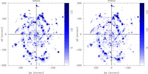
Left-hand panel: reconstructed, continuum-subtracted Hα narrow-band image of NGC 628 obtained after interpolating the aperture photometry extraction of the SINGS narrow-band image at the location of the mosaic fibres as in Fig. 4. Right-hand panel: pure Hα emission-line map of NGC 628 calculated from the IFS mosaic in units of 10−16 erg s−1 cm−2 arcsec−2. No correction for dust extinction was applied to the map. All morphological structures of the galaxy are completely reproduced in the IFS image.
Fathi07 has recently provided with a similar Hα map, with twice the FOV of our IFS data, on the basis of Fabry–Perot and complementary narrow-band images. The distribution shown by both maps is remarkably similar. They identified 376 H ii regions, many of them within the FOV of our IFS data. A detailed comparison of each of these individual sources, and an analysis of their spectroscopic properties, will be presented elsewhere (Rosales-Ortega, in preparation).
Their data confirm the presence of a central structure in NGC 628, characterized by a ring of ionized gas at ∼15–20 arcsec, already described by Wakker & Adler (1995) and Ganda et al. (2006) in their Hβ and [O iii] emission-line distributions. Fig. 10 shows a zoom-in picture of the Hα distribution already shown in Fig. 9 (right-hand panel), together with a counterplot of the continuum emission in the V band (Fig. 4, right-hand panel). The spatial resolution for this region is better than the one in the overall mosaic, due to the dithering performed only in the central pointing. The slightly oval ring structure in the ionized gas is clearly identified in the Hα map, showing a remarkable similarity with the Hβ distribution shown by Ganda et al. (2006). It is interesting to note here that despite the difference in the original sampling of the SAURON instrument (used by Ganda et al. 2006, 2007) and PPAK, the apparent resolution of both maps is very similar. This ring is detected, at different levels, in all of the emission-line spices analysed in the current article, following the same basic morphological pattern.
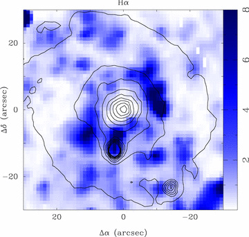
Zoom of the central ±30 arcsec region of the pure Hα emission-line map of NGC 628 calculated from the IFS shown in the previous figure. The contour plots show the continuum emission in the same region. The ionized ring described by Wakker & Adler (1995), and confirmed by Ganda et al. (2006) and Fathi07 is clearly seen.
5.2.3 Distribution of the dust attenuation
Besides the intrinsic significance of the emission-line map presented previously, the most interesting application of the 2D distribution of the different line intensities resides in the calculation of well-known line ratios that can be translated to physical properties of the emitting gas. With the aid of the IFS data we can investigate for the first time the point-to-point variation of these physical properties over a considerable area on the surface of a galaxy.
Fig. 11 shows the distribution of the dust extinction derived from the Hα/Hβ line ratio, in terms of the visual extinction AV (in magnitudes), assuming, as in the case of the analysis of the integrated spectrum, Case B recombination with an electron temperature of Te∼ 104 K, and adopting the Cardelli et al. (1989) extinction law with RV, the total to selective extinction ratio, equal to 3.1. Although other Balmer lines were detected at different locations in the galaxy, Hα and Hβ are obviously the lines with the highest S/N and therefore are the most adequate for the determination of AV. The dust extinction map was derived for those locations where the intensity of the Hβ line was above the adopted flux threshold. These regions clearly follow the spiral arm structure. The dust shows a clumpy distribution, a rich structure and large variations even within the same H ii region or complex. There is no apparent trend of the extinction along the spiral arms or in any radial direction. The average extinction derived from the values shown in the map is AV∼ 1.24 ± 0.76 mag, which is slightly larger but comparable to the value derived using the integrated spectrum (AV∼ 1.04). The reason for this discrepancy may reside in the fact that the ionized gas component of the integrated spectrum is dominated by the spectra of the outer regions, where the intensity of the emission lines is stronger and the extinction is somewhat lower. Extinctions greater than 2.5 are found in specific regions, e.g. the central zone of the giant H ii complex at ∼(–40,120), while others are found in compact H ii regions along both spiral arms. Previous studies have estimated the extinction at different locations within this galaxy targeting individual H ii regions (e.g. McCall et al. 1985; Belley & Roy 1992; Petersen & Gammelgaard 1996); the derived extinctions from these studies are consistent with the range of AV values found in this work.
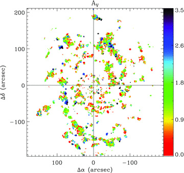
Dust attenuation map of the ionized gas (AV), derived by comparing the measured Hα/Hβ line ratio map with the expected value for case B recombination, assuming a homogeneous distribution of the electron density and temperature, and the attenuation law by Cardelli et al. (1989). The regions without accurate measurements of either emission lines were masked.
5.2.4 Ionization conditions
As discussed previously in Section 5.1.2, the source and structure of the ionization can be in principle investigated by exploring the line ratio maps of typical diagnostic indices. Fig. 12 shows on the left-hand panel the line ratio map of [N ii]λ6584/Hα (N 2 H α) and on the right-hand panel, the [O iii]λ5007/Hβ (O 3 H β) ratio map, in logarithmic scale. Note that, given the proximity of the emission lines, these indices are almost reddening independent. The N 2 H α shows a very homogeneous behaviour, with small variations in individual regions, some of them showing lower values in the central part of the regions (e.g. the knot at Δα, Δδ∼40–130). The average ratio derived from this map is −0.55 ± 0.12 dex, which is in excellent agreement with the value derived from the integrated spectrum (N 2 H α=− 0.56). However, some regions at the outer part of the galaxy show lower ratios consistent with values ∼ −0.75, e.g. (Δα, Δδ) ∼ (−50, −160), (0,200), which might suggest a gradient of this index decreasing from the inner to the outer regions of the galaxy. On the other hand, the O 3 H β shows a clear gradient along the spiral arms with lower ratios towards the inner regions and greater values at the outer part of the galaxy. The average value of this index derived from the map is −0.50 ± 0.25 dex, which again is in good agreement with the integrated value of −0.48. It is interesting to note that the regions with the highest values of O 3 H β are coincident with the zones of the lowest N 2 H α ratios. Given that the [N ii] emission originates in the singly ionized regions, between the fully ionized and the partially ionized zones, the N 2 H α ratio traces the changes in the local ionization, while the [O iii] originates in the fully ionized zones, tracing the strength of the ionization. Therefore, the distribution found in these diagnostic maps may indicate that the ionization is stronger in the outer parts of the spiral arms than in the central regions. The values of both ratios at any location in the galaxy are consistent with ionization produced by hot OB stars, as expected. In particular, there is no evidence of ionization due to shocks and/or nuclear activity.
![2D spatial properties of NGC 628, classical diagnostic line ratio maps. Left-hand panel: [N ii]λ6584/Hα line ratio map. Right-hand panel: [O iii]λ5007/Hβ line ratio map; both in logarithmic scale.](https://oup.silverchair-cdn.com/oup/backfile/Content_public/Journal/mnras/410/1/10.1111_j.1365-2966.2010.17444.x/1/m_mnras0410-0313-f12.jpeg?Expires=1749916680&Signature=PFIegTy~NYNH3AxbdPZNaOcMLvZYWau~NrzU38UfPr48EDNM2vk4uqoYVzZJ--4E8nej2G9hfZViUF~goTP2Ro5vDtGmo5o4UrTFrNTYpwRbKXPiwP1YhGQUPtztBk7GlPNr-a~4zHfyW4if~vum4Mym7yNSIFHuedCIEi3hhGUoost4-Dmi7Tb2r2Hl4rGKYa5xO-oMCRBZifpJodU5YcdAhiaau4XAUIjPSHXPdnAVafhd9IZD-nDuRMiomEjeROJy3DsYfd8t3YVMsdB8qx4GCHrG2t2qR0cH8ovi5PJKBUpqMJMyXGgKgoAqW5PpAWuuZ9Ihn3dowjsYeIO4Eg__&Key-Pair-Id=APKAIE5G5CRDK6RD3PGA)
2D spatial properties of NGC 628, classical diagnostic line ratio maps. Left-hand panel: [N ii]λ6584/Hα line ratio map. Right-hand panel: [O iii]λ5007/Hβ line ratio map; both in logarithmic scale.
An additional way of studying the 2D distribution of the galaxy properties consist in obtaining azimuthally averaged radial spectra, from which radial average properties can be derived. Taking again as a base the clean IFS mosaic version of the galaxy, radial average spectra were obtained by co-adding all the spectra within successive rings of 10 arcsec, starting from the central reference point. An average spectrum was obtained for each single annulus at a given radius. The radial average spectra were then analysed using the same fitting procedures described before. Although the derived spectra present more S/N than the single-fibre case, the measured emission lines were corrected by extinction using only the Hα/Hβ ratio for consistency with the previous method.
Fig. 13 shows the BPT diagnostic diagram (BPT) for the N 2 H α and O 3 H β line ratios. The bluish-asterisk symbols (in the online version) correspond to the derived values of the emission-line ratios for 300 randomly selected spectra distributed uniformly over the surface covered by the emission-line ratio maps shown in Fig. 12. The reddish diamonds correspond to the radial average values introduced above, while the red solid square indicates the average line ratio derived from the integrated spectrum of the galaxy. The colour coding of both the individual fibres and the radial-average samples is related to the spatial position of a given fibre/annulus. Lighter tones correspond to the inner regions of the galaxy, while darker colours correspond to positions with increasing galactocentric radius (arrow direction). The dark-thick line corresponds to the theoretical boundaries dividing the starburst region from other types of ionization using the parametrization provided by Kewley et al. (2001). The dashed lines represent the ±0.1 dex variation. As expected, the ionization is dominated by hot stars (OB class) associated with star-forming regions, at any location in the galaxy. A clear trend can be noticed in Fig. 13 for both samples, the spectra corresponding to the inner regions tend to have lower line ratios for both indices; for regions at the outer part of the galaxy, the ratios increase approaching the theoretical boundary. Part of the reason for this behaviour is that inner parts of the galaxy lack emission in [O ii] and [O iii], while towards the outer parts, the emission from these species is prominent, increasing the two line ratios involved in this diagram.
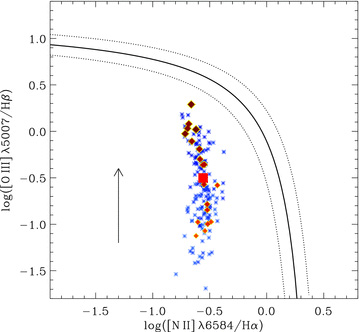
N 2 H α versus O 3 H β diagnostic diagram for NGC 628. The bluish symbols correspond to the derived values of the emission-line ratios for 300 randomly selected spectra distributed uniformly over the surface covered by the emission-line ratio maps shown in Fig. 12. The reddish diamonds correspond to the azimuthally averaged radial values. The red solid square indicates the ratio derived from the integrated spectrum of the galaxy. Lighter tones correspond to inner regions of the galaxy, darker colours to increasing galactocentric distance, outlined by the arrow. In the radial case, the size of the symbols increases with radius.
The differences in the line ratios at different locations in the galaxy may be also driven by the strength of the ionization field, being stronger in the regions with higher N 2 H α line ratio, and lower O 3 H β one. In order to investigate this point, Fig. 14 shows the distribution of the ionization parameter in logarithmic scale, log u, calculated accordingly to equation (1) (Díaz & Pérez-Montero 2000), which is based on the dust-corrected [O ii]/[O iii] ratio. Both lines were corrected by extinction using the AV map discussed previously. The log u map shows that the ionization is indeed stronger in the outer parts of the spiral arms, as the previous maps suggested. However, we can also distinguish a good degree of ionization structure in individual regions within the spiral arms, with higher values of log u corresponding to the geometrical centroids of the H ii regions, as one might expect in the scenario of a central star cluster or association embedded within an H ii region. Given that the dominant source of the ionization is radiation from OB stars, this result indicates that the SFR is stronger in the outer regions of the galaxy. A striking feature of this map is the presence of regions with low values of the ionization parameter (blue colour) located mainly in a specific region, corresponding to the first quadrant, north-west part of the galaxy. These low log u regions are found mainly at the edges of giant H ii complexes, but they are also found as individual regions. The nature of these low ionization regions will be investigated thereinafter. The mean value of log u derived from this map is −3.50 ± 0.26 dex, which is 0.08 dex higher than the value derived from the integrated spectrum of NGC 628.
![Distribution of the ionization parameter log u, in logarithm scale, derived from the dust-corrected [O ii]λ3727/[O iii]λ5007 line ratio.](https://oup.silverchair-cdn.com/oup/backfile/Content_public/Journal/mnras/410/1/10.1111_j.1365-2966.2010.17444.x/1/m_mnras0410-0313-f14.jpeg?Expires=1749916680&Signature=JOEg4GVRcAPqYMPxmvNRwYH8g8O2sdIzKL4TteXD6cLk-T9MRJkLXMXOXG~VzdJpblJgCnq79BQN0gjGQp0HW9GS7lMV95KpGeqrEdbHrTiFWy~YRohlBbjjTm2BFVz2PZyb1F20ESzo0LYxp8ucNpyLQKwlt-~ojoFnqKr~qTdwZehR55L3c9YGCvICkqWUHop9YFwjfmlhSb5p7AJJ3cHmGCg0bYJmZI5CTskWVkmX22nYtw1qEU8LCCCmJ4~edlyYDswwFt03tuqbtDQQR-GbNS6dJ12AuLBJu1NuFHxL4R-OYUQIFU06953NzUBOiFBCOWNiBXWsB7t9LuvXIA__&Key-Pair-Id=APKAIE5G5CRDK6RD3PGA)
Distribution of the ionization parameter log u, in logarithm scale, derived from the dust-corrected [O ii]λ3727/[O iii]λ5007 line ratio.
5.2.5 Surface star formation rate
The surface SFR can be derived using the emission-line distribution of Hα or [O ii]λ3727. However, the latter line suffers from more inaccuracies in both the spectrophotometric calibration and flux determination, since it lies just at the blue edge of the spectral range covered by our data set. Therefore, only the Hα intensity map was used in this analysis. Following our previous prescription to derive the integrated SFR of the galaxy, the Hα intensity map was corrected for attenuation, adopting the dust distribution described in Section 5.2.3, and the same attenuation law as in Section 5.1. Then, the dust-corrected flux densities were transformed to absolute luminosities, using the same distance and cosmology described before. These luminosities were used to obtain the surface SFR by adopting the classical relations described by Kennicutt (1998).
Fig. 15 shows the derived distribution for the surface SFR in units of 10−5 M⊙ yr−1 arcsec−2. As expected, the stronger star formation is distributed in clumps along the spiral arms, following a similar morphology to the distribution of the Hα emission (i.e. the H ii regions). In addition, the direct transformation between extinction-corrected Hα flux and SFR produces an apparent, low-level, SFR in the inter-arms regions, two orders of magnitude lower than that of the H ii regions. However, it is unclear how closely associated is this derived SFR with the inter-arm Hα emission. Ionizing photons leaking from the H ii regions and stochastics in the conversion between both parameters may become important at this intensity level. As already shown by the distribution of the N 2 H α and O 3 H β line ratios (Fig. 12), and the ionization parameter (Fig. 14), there is an increase of the SFR from the inner to the outer regions of the spiral arms.
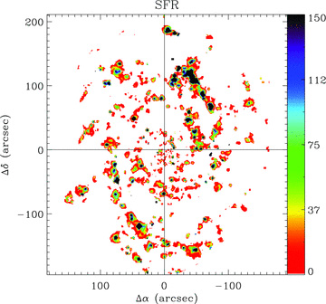
Surface SFR in units of 10−5 M⊙ yr−1, derived from the Hα line intensity map shown in Fig. 10, after correcting by dust attenuation. This map traces the distribution of the ionized gas, not the young stars, which form much more compact structures than the ones shown in the figure.
The global SFR can be derived by co-adding the surface SFR over the area shown in the figure, obtaining a value of ∼1.1 M⊙ yr−1. By applying the same aperture and sampling correction applied to the integrated Hα flux in Section 5.1, the estimated SFR is ∼2.4 M⊙ yr−1, which is practically identical to the estimate derived based on the flux of Hα in the integrated spectrum.
5.2.6 Distribution of the gas-phase oxygen abundance
One of the main purposes of the PINGS data set is to study the metallicity content of the galaxy in a 2D context. As discussed previously, the oxygen abundance is normally derived using a variety of diagnostic methods based on strong lines, from which the most common one is the R23 indicator. The dust-corrected emission-line maps of [O ii] and [O iii] provide the means to explore the behaviour of this indicator. The left-hand panel of Fig. 16 shows the R23 map of NGC 628. From a first visual inspection, it is evident that the map presents a clear gradient of lower values of R23 in the inner regions of the galaxy, to higher values to the outer parts, specially along the spiral arms. The average R23 value derived from the map is 2.41 ± 1.37, which is in good agreement with the value inferred from the integrated spectrum (R23 = 2.57). The lower values of R23 in the central regions of the galaxy are expected, given the low emission of [O ii] and (especially) [O iii], as inferred in figure Fig. 13. For well-defined H ii regions, the value of R23 seems to be constant in the majority of the cases; however, there are regions in which the value of R23 varies within the H ii region or complex, showing some level of structure. Considering the O/H values derived after different calibrators from the integrated spectrum of NGC 628 in Section 5.1.3 (12 + log(O/H) ∼ 8.7), and previous abundance determinations from individual H ii regions in this galaxy (e.g. McCall et al. 1985; Ferguson et al. 1998), suggest that the average oxygen abundance of NGC 628 corresponds to the high-metallicity regime. In this scenario, the double-valued nature of the R23 index can be broken, and the gradient of higher-to-lower values of R23 from the inner to the outer parts of the galaxy shown in this map would correspond to the decrement of the R23 ratio in the upper-branch of a O/H versus R23 diagram, and therefore, to a true metallicity gradient of the galaxy, as previous studies based on individual H ii regions have shown.
![2D distribution of the R23 and [O iii]/[N ii] metallicity indices for NGC 628. Both maps show a gradient of lower values in the inner regions to higher values to the outer part of the galaxy.](https://oup.silverchair-cdn.com/oup/backfile/Content_public/Journal/mnras/410/1/10.1111_j.1365-2966.2010.17444.x/1/m_mnras0410-0313-f16.jpeg?Expires=1749916680&Signature=m2jyNNWcL1tshp019-J0vMzp3xyQTMgGvfSiT3e0x5fEVWumt6O-gQbXMeTpilz3JwzrpRSltb15~1eUUZ7BInLUZ4ALvUQIz-r~eHHrEec9pzNe-uyGJh6G96reS5WQ-GCuMWSB2cPjXcuqoBMTcfxU0v3seIuS8Q1Zl7GKClt8w36jHz9k4gNNZae4jFQW95Tzi-9nRmt3pnfW1Oxd3MXe9OVmeeCLktzNzFe0r4SdrlZ2LHTiQJUmA4Ne47aoC5TEDbdI7CL9860czh90-EwuVsIQnSryx7kEkc9EDsJY13Oo1lH9pFBFd-7lJ8In01DuBKBmBu4-mxt73uMy-Q__&Key-Pair-Id=APKAIE5G5CRDK6RD3PGA)
2D distribution of the R23 and [O iii]/[N ii] metallicity indices for NGC 628. Both maps show a gradient of lower values in the inner regions to higher values to the outer part of the galaxy.
Another popular metallicity-sensitive index is given by the [O iii]λ5007/[N ii]λ6584 ratio. Pettini & Pagel (2004) suggested the use of this ratio (in a modified version) as abundance indicator suitable for the analysis of high-redshift galaxies. However, the direct application of this indicator may be too simplistic, the reasons being that the [O iii]/[N ii] ratio is strongly dependent on the excitation of the nebula, and it is also sensitive to both the ionization parameter and to the age of the cluster of exciting stars (Dopita et al. 2000). As suggested by Dopita et al. (2006), the [O iii]λ5007/[N ii]λ6584 ratio can only be used as an abundance indicator only when a characteristic age of the exciting clusters can be assumed, and its application in single galaxies should be taken with caution. However, the combination of this ratio with, for example, the [N ii]λ6584/[O ii]λ3727 ratio can provide a good diagnostic of both metallicity and age of the ionizing source (Dopita et al. 2006). The right-hand panel of Fig. 16 shows the map of the [O iii]λ5007/[N ii]λ6584 ratio of NGC 628 in logarithmic scale. It is worthy to note that this ratio spans for more than two orders of magnitude. Similarly to the R23 map, this panel shows a gradient of lower values of the [O iii]/[N ii] ratio from the inner part of the galaxy, to higher values in the outer parts. The average value derived from the map is −0.35 ± 0.36 dex, compared to −0.40 obtained from the integrated spectrum. The map shows a smoother distribution within individual regions compared to the R23 map. With the corresponding cautions considering the known dependences of this index with the functional parameters of the H ii regions, the [O iii]/[N ii] gradient found for NGC 628 would correspond to a metallicity gradient of the galaxy, with some level of inhomogeneity in individual regions as shown in this map. In order to determine the existence of abundance variations within the same region of the galaxy, it would be required to co-add the spectra corresponding to regions with similar ionization conditions, and then perform an analysis based on single regions. This detailed analysis, together with a complete study of the radial abundance gradient of this galaxy, will be presented in a forthcoming paper (Rosales-Ortega et al., in preparation).
In Fig. 17, we present the oxygen abundance 2D map of NGC 628 based on the O3N2 calibrator in units of 12 + log(O/H), obtained by the manipulation of the emission-line maps presented before. No other 2D abundance maps were attempted since the parametrizations of the different calibrators do not allow a simple image manipulation (large blank areas produce convergence problems which limits the application of any interpolation routine). However, as discussed previously in Section 5.1.3, the O3N2 abundance determination qualitatively follows the same pattern as the other more elaborated calibrators based on R23 and the ff–Te relation. The map of Fig. 17 shows a clear gradient of higher oxygen metallicity values from the inner part to the outer part of the galaxy, and along the spiral arms. The most metal-deficient regions are found at the extremes of the spiral arms; a prominent region is found at (Δα, Δδ) ∼ (−40, −60). The average value of the oxygen abundance derived from this map is 8.75 ± 0.17, which is equivalent to the oxygen abundance derived from the integrated spectrum using the same calibrator, i.e. 8.71 ± 0.11.
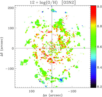
Oxygen abundance map of NGC 628 derived by applying the O3N2 calibrator (Pettini & Pagel 2004) to the emission-line maps of the galaxy. The figure shows a clear gradient in metallicity, with more abundant regions in the inner part of the galaxy.
6 DISCUSSION AND CONCLUSIONS
In this article, we presented wide-field IFS observations of a substantial fraction of the nearby galaxy NGC 628 (∼70 per cent of its projected optical size). The observations were performed by adopting a mosaicking procedure, using the PPAK IFU (mounted at the 3.5-m telescope at Calar Alto), which provides a sampling of 2.7 arcsec and an FOV larger than 1 arcmin (diameter). The total data set comprises 11 094 individual spectra, covering a nearly circular FOV of ∼6 arcmin in diameter, centred on the bulge of the galaxy. To our knowledge, this is the largest spectroscopic survey ever made of a single nearby galaxy. A detailed flux calibration technique has been applied, which granted a spectrophotometric accuracy of ∼0.2 mag, down to a surface brightness of ∼22 mag arcsec−2, comprising 6949 spectra from the original data set.
The spectrophotometrically calibrated data have been analysed both as a single integrated spectrum, which characterizes the global properties of the galaxy, and using each individual spectrum to determine the spatial variation of galaxy properties. The stellar and ionized gas components have been decoupled by a fitting technique which uses SSP templates and single Gaussian functions, respectively, to characterize these components. The main properties extracted from the analysis of the stellar continuum emission were the luminosity-weighted ages, metallicities and dust attenuation of the composite stellar population. On the other hand, for the gas content, we derived the morphology of the ionized gas, the dust content, the spatially resolved SFR, the source of the ionization and the oxygen abundance.
Table 7 lists the main properties derived in this study for NGC 628. For each of the estimated parameters we list the values derived based on the analysis of the integrated spectrum (labelled as Integrated), and the average values derived from the 2D maps (labelled as Average). When more than one technique was used to derive the values, we listed the values derived using the same technique for both data sets. In all cases, the derived values are compatible.
Summary of the main properties of the galaxy.
| Parameter | Integrated | Average |
| Age (Gyr) | 8.95 | |
| [Z/H] | −0.44 | |
| AV stellar (mag) | 0.4 | |
| AV (mag) | 1.04 | 1.24 ± 0.76 |
| log ([N ii]λ6584/Hα) | −0.56 | −0.55 ± 0.12 |
| log ([O iii]λ5007/Hβ) | −0.48 | −0.50 ± 0.25 |
| log u | −3.58 | −3.50 ± 0.26 |
| SFR (M⊙ yr−1) | 2.4 | 2.4b |
| log R23 | 0.41 | 0.38 ± 0.13 |
| log ([O iii]λ5007/[N ii]λ6584) | −0.40 | −0.35 ± 0.36 |
| 12 + log(O/H)O3N2 | 8.71 ± 0.11 | 8.75 ± 0.17 |
| 12 + log(O/H)a | 8.69 ± 0.31 |
aMean abundance among the various empirical calibrators.
bCo-added.
Regarding the spatial distribution of the different analysed properties, a gradient was found in the luminosity-weighted age of the stellar populations from the central regions, having older stellar populations, to the outer regions, having younger components. On the other hand, the radial dependence of the stellar metallicity is weaker, showing a slight or no gradient. If there is any gradient, the richer stellar populations are located at the central regions, while the poorer ones are at the outer regions. All together these results are consistent with our current understanding of how the late-type galaxies grow along cosmological epochs, that is inside-out (Barden et al. 2005). The older and more metal-rich stellar populations, formed before, on the basis of recycled gas from previous populations, are located in the centre, while the younger and less metal-rich stars are in the outer regions. It is interesting to note that the oxygen abundance in the ionized gas follows nearly the same distribution (Fig. 17), with larger abundances in the inner regions and lower abundances in the outer ones. This gradient was previously reported by McCall et al. (1985), and confirmed by Belley & Roy (1992), van Zee et al. (1998) and Ferguson et al. (1998).
In the case of the stellar populations, there seems to be an inversion of the age gradient at the very centre of the galaxy (∼1 kpc), where apparently there exist a ring of old stars at this distance, with a trend to younger ones at the very centre. These results were previously reported by Ganda et al. (2007), on the basis of their IFS observations at the very centre of this galaxy. Similar results have been reported in other galaxies, mostly Sa/S0, where the inner regions of their bulges present bluer colours, consistent with younger stellar populations (e.g. Deharveng et al. 1997). According to this scenario, the circumnuclear star formation rings detected in Sa-Sbc galaxies might show evidence of gas transfer due to radial motions in these galaxies (e.g. Knapen et al. 2006).
Spatially resolved maps of the emission-line intensities and physical properties were derived for NGC 628. Contrary to previous attempts to perform a 2D wide-field analysis based on narrow-band (or Fabry–Perot) imaging, which only allowed a basic analysis of the physical parameters and/or required assumptions on the line ratios included within individual filters (e.g. Hα), the emission-line maps presented in this paper were constructed from individual (deblended) emission lines at any discrete spatial location of the galaxy, where enough S/N was found. This fact allowed us to investigate the point-to-point variation of the physical properties over a considerable area on the galaxy. Extinction, ionization and metallicity-sensitive indicator maps were derived from reddening corrected emission-line maps. In general, they show that the ionized gas in these spiral galaxies exhibits a complex structure, morphologically associated with the star-forming regions located along the spiral arms.
In general, it is found that the dominant ionization process is due to the OB hot stars associated with star-forming regions, based on the distribution of the classical diagnostic lines. The ionization is stronger along the spiral arms, associated with the H ii regions, and more intense in the outer than in the inner ones. Indeed, the surface SFR is an order of magnitude stronger in the outer H ii regions, at distance larger than ∼100 arcsec (4.5 kpc), than in the inner ones. Considering that in these outer regions there is a lower mass density, the growing rate of stellar mass is considerably larger there than in the inner ones. Therefore, even taking into account the circumnuclear SFR, the growth of the galaxy is dominated by the inside-out process.
There is growing evidence of a central structure in NGC 628, widely discussed by Fathi07. This structure is characterized by a ring of ionized gas (Wakker & Adler 1995; Ganda et al. 2006; Fathi07), and a drop in the B−V colours (Natali et al. 1992; Fathi07). The kinematic analysis of the stellar and gas component within this ring, in comparison with that of the rest of the galaxy, indicates that there is a rapidly rotating component, most probably a dynamically cold disc, which could be built by the inflow from the outer parts towards the centre (Daigle et al. 2006; Ganda et al. 2006; Fathi07). Fathi07 found that this circumnuclear ring is located at the expected distance of the inner resonance radius (Lindbald 1961). At this location the gas tends to accumulate, due to non-circular motions exerted by a bar or spiral arms. This gas concentration may lead to a low-luminosity starburst (e.g. Knapen et al. 1995). Our results show, for the first time, that (1) the gas in the circumnuclear ring is ionized by star formation, and (2) the ring is spatially coincident with a decrease in the luminosity-weighted ages of the stellar populations, which causes the previously observed drop in the B−V colours. All together, they support the interpretation outlined by Fathi07.
The integrated spectrum of the galaxy was used to analyse the chemical abundance of the galaxy by means of different empirical diagnostic abundance calibrators. We confirmed the validity of the determination of the integrated chemical composition of a galaxy through the analysis of the global-emission-line spectra, as previously found by other authors (Kobulnicky et al. 1999; Pilyugin et al. 2004; Moustakas & Kennicutt 2006a), under the assumption that the observed emission lines arise via photoionization from young, massive stars. From the set of calibrators used for this purpose, the R23 methods based on photoionization modelling provide higher values of the oxygen abundance (i.e. M91 & KK04), followed by those methods which consider one of two emission-line indices (N2, O3N2) and the ff–Te method. The differences between different calibrators are as large as ∼ ±0.7 dex, especially for the high values of O/H derived from the R23 methods compared to the other ones. If an arbitrary negative offset is applied (as suggested by the literature), the O/H values seem to be consistent for an average integrated oxygen abundance of NGC 628 of 12 + log(O/H) ∼ 8.7, in agreement with previous studies. Note that the validity of the abundance determination depends mainly on the chosen calibrator used to derive the chemical composition, and to a second order, on the SSP fitting decoupling.
The spatially resolved distribution of the abundance shows a clear gradient of higher oxygen metallicity values from the inner part to the outer part of the galaxy, and along the spiral arms (Fig. 17). However, in some instances, the value of the oxygen abundance (and other physical properties like extinction and the ionization parameter) varies within what would be considered a classical well-defined H ii region (or H ii complex), showing some level of structure. Indeed, the 2D character of the PINGS data allows us to study the small-scale variation of the spectra within a given emitting area. As suggested in Paper I, the values of the emission-line ratios measured using different extraction apertures vary considerably as a function of the aperture size, and that the scatter of the central value is larger than the statistical error in the measurements, reflecting that this might in fact be a physical effect. If we take as a premise that for a sufficiently large H ii region, the emission-line measurements are aperture and spatial dependent, i.e. that the light is emitted under different physical conditions, by gas in different degrees of ionization, and modified by different amounts of reddening (and therefore providing different elemental ionic abundances), the level of structure seen in the 2D maps of NGC 628 may be due to the intrinsic distribution of the ionizing sources, gas content, dust extinction and ionization structure within a given region, i.e. we would be sampling real point-to-point variations of the physical properties within a H ii region.
The emission-line maps presented in this paper proved to be useful in describing the general 2D properties of the selected galaxies. However, the conclusions raised from them were based on general trends that depend, to a certain level, on the interpolation scheme applied in order to derive the pixel-resolved maps. More robust conclusions can only be drawn by analysing specific individual regions within the given galaxy, or by co-adding spectra of regions with the same physical properties and comparing the results in the 2D context. This approach will be followed in subsequent papers in order to study the spatially resolved spectroscopic properties of this and the rest of the PINGS galaxies.
The Digitized Sky Survey was produced at the Space Telescope Science Institute under U.S. Government grant NAG W-2166. The images of these surveys are based on photographic data obtained using the Oschin Schmidt Telescope on Palomar Mountain and the UK Schmidt Telescope. The plates were processed into the present compressed digital form with the permission of these institutions.
iraf is distributed by the National Optical Astronomy Observatories, which are operated by the Association of Universities for Research in Astronomy, Inc., under cooperative agreement with the National Science Foundation.
N. Cardiel, http://tinyurl.com/rmodel
Accessible at http://www.ast.cam.ac.uk/research/pings/html/public/
SFS thanks the Spanish Plan Nacional de Astronomía programme AYA2005-09413-C02-02 of the Spanish Ministry of Education and Science and the Plan Andaluz de Investigación of Junta de Andalucía as research group FQM306 and the ARAID foundation for providing funds.
SFS thanks the director of CEFCA, Dr M. Moles, for the unconditional support to this project.
FFR-O would like to thank the Mexican National Council for Science and Technology (CONACyT) and the Dirección General de Relaciones Internacionales (SEP-México). We would like to thank the referee, R. Peletier, for the very valuable comments and suggestions which improved the final content of this paper. We acknowledge Dr N. Cardiel for his help in the study of the stellar populations.
REFERENCES
Appendix
APPENDIX A: MULTIPLE-STELLAR POPULATION FITTING
A substantial fraction of the stellar continuum emission in early-type galaxies is dominated by a SSP, reflecting the fact that their cosmological evolution is, in many cases, well described by a monolithic collapse model. In this scenario most of the star formation took place in these galaxies for a short time at early times, and therefore, their SFH can be well described by a single star formation process. As a consequence, their stellar continuum can be easily described by a single-stellar population.
It is well known that the SED of simple stellar populations (chemically homogeneous and coeval stellar systems) depends on a set of first principles (e.g. initial mass function, SFR, stellar isochrones, metallicity, etc.), from which it is possible to generate the spectra of synthetic stellar populations. This technique, known as evolutionary synthesis modelling (e.g. Tinsley 1980), has been widely used to unveil the stellar population content of galaxies by reconciling the observed SEDs with those predicted by the theoretical framework. Unfortunately, the variation of different physical quantities governing the evolution of stellar populations produces similar effects in the integrated light of those systems, leading to a situation in which the observational data are affected by undesirable degeneracies, like the widely mentioned one between age and metallicity (e.g. Oconnell 1976; Aaronson et al. 1978; Worthey 1994). However, the use of spectrophotometrically calibrated spectra and the sampling of a wide wavelength range, as in the present data set, helps in breaking the degeneracy and allows the derivation of reliable physical parameters by fitting the full spectral distribution with SSPs (Cardiel et al. 2003).
However, the simple assumption that a SSP describes well the SED of a galaxy is not valid for late-type galaxies. These objects present complex star formation histories, with different episodes of activity, of variable intensity and time-scale. Therefore, a SSP does not reproduce well their stellar emission, in general terms. A different technique, known as full-spectrum modelling, involving the linear combination of multiple stellar populations and the non-linear effects of dust attenuation, has been developed to reconstruct their stellar populations (e.g. Fernandes et al. 2005; Ocvirk et al. 2006; Sarzi et al. 2006; Koleva et al. 2009; MacArthur et al. 2009).
In general, these reconstructions require a wide wavelength range to probe the hot, young stars and the cool, old stars simultaneously. They also require the best spectrophotometric calibration to disentangle the effects of age, metallicity and dust attenuation. Although different implementations of this technique have some differences, they are very similar in their basis, as described above. The extracted information from the multi-stellar-population modelling differs in the different implementations. In some cases the luminosity (or mass) weight ages and metallicities are derived, based on the linear combination of different models (e.g. Sarzi et al. 2006). In other implementations the fraction of light (or mass) of different stellar populations (e.g. Stoklasová et al. 2009), or the fraction of light (or mass) that corresponds to old or young stellar populations (e.g. MacArthur et al. 2009), are derived.
For our particular analysis, it is necessary to accurately model the underlying continuum not only to understand the nature of the stellar population, but also to obtain a good representation of the continuum in order to decouple it from the emission lines produced by the ionized gas. Therefore, even in the case that the combination of SSPs is strongly degenerate, and the created model has no physical meaning, it could be partially useful for our purposes.
The implementation of the multi-stellar-population fitting technique used in this article is part of the fit3d package (e.g. Sánchez et al. 2007b,c), and it has been recently used by e.g. Stoklasová et al. (2009) in the analysis of the stellar population of nearby galaxies based on IFS data. This package enables linear fits of a combination of SSPs, and non-linear ones of emission lines plus an underlying stellar population. It also includes routines to extract the 2D distribution of the different derived parameters based on the analysis of the stellar population (age, metallicity, dust) and/or the analysis of the emission lines (flux intensity, systemic velocity and velocity dispersion). The package will be delivered to the public in a forthcoming paper. The basic steps of the fitting algorithm, spectrum by spectrum, are the following.
Read the input spectrum, determine the areas to be masked and construct the variance map. Let us define Gi as the observed galaxy flux at wavelength λi, and N the number of elements of the masked spectrum.
Read the set of SSP template spectra, shift them to the systemic velocity of the considered spectrum, convolve them to match its spectral resolution and velocity dispersion, and resample them to its wavelength solution. Lets define Fji as the flux of the ith wavelength of the jth template (once shifted, convolved and resampled), where M0 is the total number of considered templates.
Apply a certain dust attenuation to the templates. The attenuation law of Cardelli et al. (1989) was adopted, with a ratio of total to selective attenuation of RV = 3.1 (Jenkins 1987). Let us define
 as the flux of the ith wavelength of the jth template, after applying the dust attenuation corresponding to a certain attenuation of AV magnitudes.
- Perform a linear least-square fitting of the input spectrum with the set of SSP templates, using a modified χ2 as a merit function to be minimized, with the formwhere

 In the above expression, wi is the weight of the ith pixel, defined asand aj is the coefficient of the jth template in the final modelled spectrum, and M is the number of templates considered in the fitting procedure.
Determine for which templates the fitting procedure produces negative coefficients in the linear combination (i.e. aj < 0). These templates will be excluded from the next iteration of the fitting procedure, that will be resumed in Step (iii). At each iteration, M is decreased by the amount of excluded templates. This loop ends once all the coefficients are positive.
The modified χ2 corresponding to the considered dust attenuation is stored as
 , and the fitting procedure is repeated again starting at Step (iii), modifying the considered amount of dust and starting the procedure with the full set of templates (i.e. M=M0, again). The loops finish once the dust attenuation has covered a pre-defined range of values, that it is defined as an input parameter.
- The best linear combination of templates and dust attenuations is selected based on the minimization of the stored χ2 parameters. The final modelled spectrum flux at λi is given bywhere in this case only the M templates with positive coefficients aj are considered, and AV corresponds to that value which minimizes

 .
. - The luminosity-weighted age (H) and metallicity (Z) of the underlying stellar population are then derived by the formulaeand
 where Hj and Zj are the corresponding age and metallicity of the jth SSP template. These luminosity-weighted ages and metallicities should be considered as the luminosity-weighted ages and metallicities of the modelled stellar population, since they would match with the corresponding values if the population was composed by a single SSP.
This algorithm shares a basis with many other procedures described in the literature (e.g. Fernandes et al. 2005; Sarzi et al. 2006, MacArthur et al. 2009). If required, low frequencies in the spectrum can be fitted by adding to the fitted templates a polynomial function, or by multiplying them by that function. There are of different origins for these low frequencies in the spectrum, mostly related with defects in the reduction process. In the particular case of the data analysed in the current article, the inclusion of this additional step in the fitting procedure does not considerably improve the results.
By construction, the fitting algorithm is useful for masking undesirable regions in the spectrum. In general, it is needed to mask: (i) strong and variable night sky-line regions, (ii) regions affected by defects in the CCD (like dead columns) whose effect was not completely removed during the data reduction process, (iii) regions affected by telluric absorption, not completely corrected during the flux calibration process and (iv) regions containing emission lines from ionized gas.

A1 Modelling the emission lines
To derive the intensity of each detected emission line, the clean spectrum (Ci) is fitted to a single Gaussian function per emission line plus a low-order polynomial function. This fit is performed using non-linear fitting routines implemented in fit3d that were described in the previous articles. Instead of fitting all the wavelength range in a row, we extracted for each spectrum shorter wavelength ranges that sampled one or a few of the analysed emission lines, in order to characterize the residual continuum with the most simple polynomial function, and to simplify the fitting procedure. When more than one emission was fitted simultaneously, their systemic velocities and FWHMs were forced to be equal (since the FWHM is dominated by the spectral resolution), in order to decrease the number of free parameters and increase the accuracy of the deblending process (when required). These procedures are frequently used, and therefore, we will not explain them in more detail.
This spectrum is then used to model the stellar population, by applying the procedure described before, but without masking the emission lines spectral regions. We adopted the results from this second iteration as a better modelling of the stellar population.
A2 SSP template library
As noted by MacArthur et al. (2009), this kind of analysis is always limited by the template library, which comprises a discrete sampling of the SSP ages and metallicities. It would be desired for the stellar library to be as complete as possible, and non-redundant. However, this would require an exact match between the models and the data, which is not possible to achieve in general terms, in particular if the stellar population comprises more than one SSP. As a suitable solution for the analysis presented in this article, we adopted an SSP template library that covers the widest possible range of ages and metallicities. This template has already been demonstrated as useful for modelling the stellar population of a varied set of galaxies (see Sánchez et al. 2007c).
The SSP models were created using the gissel code (Bruzual & Charlot 2003), assuming a Salpeter IMF (Salpeter 1955) (the use of Chabrier 2003, will not modify the results), for different ages and metallicities. We create 72 models covering a discrete grid of 12 ages (5 Myr, 25 Myr, 100 Myr, 290 Myr, 640 Myr, 0.9 Gyr, 1.4 Gyr, 2.5 Gyr, 5 Gyr, 11 Gyr, 13 Gyr and 17 Gyr), and six metallicities (Z=0.0001, 0.0004, 0.004, 0.008, 0.02 and 0.05). Fig. A1 shows the spectra of all the templates, grouped by their metallicity, and normalized to their flux at 5000 Å. The adopted library is similar in many respects to the one proposed by MacArthur et al. (2009). Both libraries have a similar number of templates, although the latter library has a wider coverage of the ages and a more reduced coverage of the metallicities of the stellar populations.
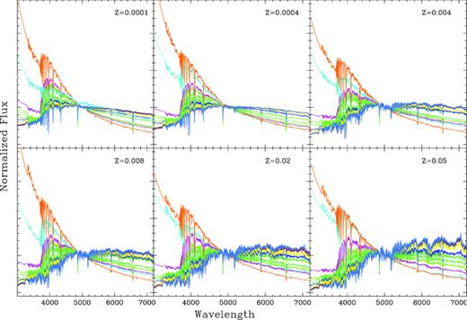
Spectra of the 72 SSP templates used in the population synthesis fits. Metallicity increases from the top left to the bottom right. Different ages are represented by different colours. All the spectra are normalized to the flux at 5000 Å.
There are a number of caveats when applying model SSPs to the integrated light of a star-forming galaxy, which have been clearly identified by MacArthur et al. (2009). The most important one is to assume that the parameter space covered by the empirical library represents well that of the real data. However, in general, libraries are based on stars in the solar neighbourhood, and therefore it is not granted that they represent well the stellar populations in other galaxies (or even in other regions of our Galaxy). There are other potential problems related to the particular selected templates, since it is well known that the Bruzual & Charlot (2003) models have problems when dealing with the non-solar abundance ratios. Most of these problems are not particularly important in the context of our science case, since (i) our primary goal is to model the stellar population to analyse the ionized gas emission and (ii) we are interested in relative assessments about the nature of the stellar populations in different regions of the studied galaxy, and not in absolute values.
In addition, it is important to note that the treatment of the dust attenuation may affect the resulting derived parameters (i.e. the luminosity-weighted age and metallicity of the stellar population). In this particular implementation of the analysis we adopted the Cardelli et al. (1989) attenuation law, which may not be the optimal solution to study the dust attenuation in star-forming galaxies (e.g. Calzetti 2001). MacArthur et al. (2009) adopted a completely different attenuation law, based on the two-components dust model of Charlot & Fall (2000), which is particularly developed to model the dust attenuation in star-forming galaxies. Despite the conceptual differences between the two attenuation laws, their actual shapes are very similar in the wavelength range covered by our data. The final range of dust attenuations explored by our fitting technique comprises AV values up to 1 mag, with steps of 0.1 mag.
A3 Accuracy of the derived parameters
As mentioned before, the basic parameters derived by the analysis of the stellar component are the luminosity-weighted age, metallicity and dust attenuation of the composite stellar population. In order to assess the accuracy of these parameters we have performed a set of simulations. The simulations were performed while trying to match as closely as possible the original data, especially the noise pattern, which is composed of both white noise corresponding to the photon-noise of the source and the background, and electronic noise from the detector and non-white noise corresponding to defects/inaccuracies in the sky-subtraction, uncorrected defects in the CCD, etc. These noise patterns are different from spectrum to spectrum, and wavelength to wavelength, and are clearly difficult to simulate on a simple analytical basis.
Five different sets of simulations were performed. In each one, 500 simulated spectra were created with the same normalized flux at 5000 Å, corresponding to 100, 10, 5, 1 and 0.2 × 10⁻¹⁶ erg s−1 cm−2 Å−1, respectively. For each simulation, a composite stellar population was considered, comprising four different SSP extracted randomly from the considered library template, with a different relative contribution from each one to the total flux: 53 per cent, 27 per cent, 13 per cent and 6 per cent at 5000 Å, respectively. This procedure was adopted to resemble in a simple way a possible star-forming history, with a dominant stellar population, and three different bursts or merging events. Different experiments adopting a larger number of intermix stellar populations, and relative contributions of each one to the total, were considered, with no significant variations on the derived conclusions.
Once a particular spectrum was created, it was convolved with the instrumental resolution of the observed data, and the corresponding noise pattern was added. The noise pattern was created on the basis of the residuals of the fitting procedure applied over the observational data. For each spectrum of the original mosaic, the fitting procedure creates a residual spectrum, once the derived composite stellar population and emission-line models were subtracted. This noise spectrum includes all the effects of the white noise (for a particular flux level), and non-white noise (deficient sky subtraction, CCD defects not corrected by the reduction, imperfections of the modelling process, etc.). From this set of noise spectra, one was randomly selected for each simulated spectrum, fulfilling the requirement that the simulated and original fluxes at ∼5000 Å match within a range of ∼20 per cent. The selected noise spectrum was then added to the simulated spectrum.
The fitting procedure was then applied to the simulated spectra using the same steps adopted to analyse the observational data, deriving, for each one, the luminosity-weighted ages, metallicities and dust attenuation, and a new residual spectrum. Table A1 lists, for each set of simulated spectra, their average S/N, the rms of the relative difference between the input spectra (without noise) and the model derived by the fitting procedure and the difference between the input and the recovered parameters that define these models (luminosity-weighted age, metallicity and dust attenuation), and their corresponding rms. As expected the parameters are better recovered for the spectra with higher S/N, requiring at least a S/N of ∼50 per pixel to derive accurate results. Fig. A2 illustrates these results, showing for each set of simulations the comparison between the input and recovered parameters for each individual spectrum in the data set.
Results of the simulations.
| S/N | rms | ΔAge/age | ΔZ | ΔAV |
| 734.60 | 0.14 | 0.02 ± 0.14 | 0.0001 ± 0.0014 | 0.00 ± 0.05 |
| 90.28 | 0.11 | −0.03 ± 0.24 | 0.0006 ± 0.0047 | 0.01 ± 0.08 |
| 43.74 | 0.11 | −0.08 ± 0.30 | 0.0004 ± 0.0074 | 0.03 ± 0.13 |
| 8.60 | 0.12 | −0.18 ± 0.46 | 0.0014 ± 0.0126 | 0.04 ± 0.38 |
| 1.69 | 0.12 | −0.18 ± 0.59 | 0.0006 ± 0.0164 | −0.06 ± 0.51 |
| 82.77a | 0.12 | 0.21 ± 0.27 | 0.0010 ± 0.0070 | −0.01 ± 0.10 |
| 81.97b | 0.13 | 0.12 ± 0.47 | 0.0023 ± 0.0075 | −0.01 ± 0.23 |
aResults when fitting the simulated spectra with a different library of SSPs than the one used to create the simulation.
bResults when the input simulated spectra consist of a single SSP, instead of a combination of them.
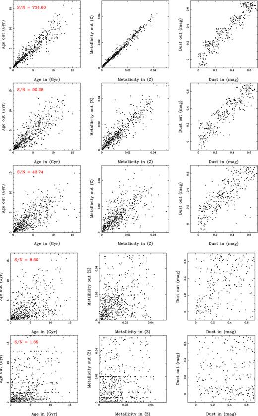
Results from the simulations. Each panel shows, from left to right, the comparison between the input luminosity-weighted age, metallicity and dust attenuation, with the recovered values by our fitting technique. The results are presented for different S/N, decreasing from the upper to the lower panels. A random value of ±0.08 mag has been added to output attenuation to show all the values, since they are originally quantized to steps of 0.1 mag.
A possible source of error in the interpretation of these simulations is the fact that the same set of templates was used to create the simulated data and to model them. In principle, we assumed that the grid of templates is representative of the real stellar population of the analysed spectra, but it is very possible that our library is incomplete. This is not the case in our simulations, by construction. To study the effects of this possible incomplete representation of the observational spectra by the template library, we created a new set of simulated data, corresponding to a flux level of 10 × 10−16 erg s−1 cm−2 Å−1, that was then fitted using a much reduced version of the template library. This template comprises a grid of 12 SSPs, corresponding to three ages (17 Gyr, 900 Myr and 25 Myr) and four metallicities (Z = 0.0001, 0.004, 0.02, 0.05). The results from this simulation are listed in Table A1, and are shown in Fig. A3. It shows that in the case of an incomplete coverage of the spectroscopic parameters by the model template, these parameters are still well reconstructed, albeit with a lower accuracy (as expected).
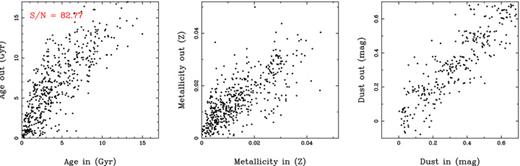
Results from the simulations. Each panel shows, from left to right, the comparison between the input luminosity-weighted age, metallicity and dust attenuation, with the recovered values by our fitting technique. The difference from Fig. A2 is that in this particular case, a different library of SSPs was adopted to fit the spectra, compared to the one used to simulate them, as described in the text.
Finally, we tested how well the code is able to reproduce a pure SSP, instead of a mixture of them. With this test we try to overpass the intrinsic problems in the interpretation of the luminosity-weighted ages/metallicities in galaxies, and to test if we can recover the better understood properties of a pure single-burst population. The results from this simulation are listed in Table A1, and shown in Fig. A4. Despite the discrete coverage of the input parameters, it is clear that the parameters are recovered just slightly worse than in the case of a multiple component stellar population.
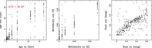
Results from the simulations. Each panel shows, from left to right, the comparison between the input luminosity-weighted age, metallicity and dust attenuation, with the recovered values by our fitting technique. The difference from Fig. A2 is that in this particular case, the input model consists of a single SSPs, although it is fitted following the prescriptions shown in the text.
On the other hand, the relative difference between the original spectra and the recovered model is lower than ∼15 per cent for all the simulations, even in those for which the accuracy of the recovered parameters is deficient. These differences are of just 2–3 per cent for the spectra with the highest S/N (>100). This basically means that the general shape of the spectra is better recovered than the parameters that define them. This is easy to understand, since these parameters are characterized by particular features in the spectra, rather than by their general shapes, which are more degenerated.
Fig. A5 shows the radial distribution of the average S/N at ∼5000 Å of the spectra within the flux-calibrated mosaic of NGC 628, as described in Section 3. On the basis of this radial profile and the results of the simulations discussed before, it is possible to recover the considered parameters of the composite stellar populations for individual spectra only at radii less than ∼10 arcsec, for the central kpc of the galaxy. The results are robust only for the integrated spectrum of the galaxy (with a S/N ∼ 400), and for radii lower than ∼20 arcsec (with S/N ∼ 100). However, for the azimuthally averaged spectra, where the S/N increases by the rms of the number of individual averaged spectra, the simulations indicate that the recovery of the considered parameters is robust even at radii as large as ∼120 arcsec, above which both the S/N and the number of spectra with accurate spectrophotometry also drop (see Fig. 4). The combination of both effects imposes a limitation to the accuracy of the derived parameters at higher radii.
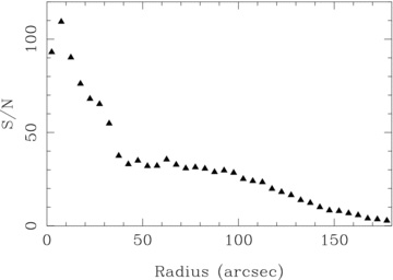
Radial distribution of the average S/N at ∼5000 Å of the spectra within the flux calibrated mosaic of NGC 628.
Author notes
Based on observations collected at the Centro Astronómico Hispano Alemán (CAHA) at Calar Alto, operated jointly by the Max-Planck Institut für Astronomie and the Instituto de Astrofísica de Andalucía (CSIC).
