


Abstract
We report the first calculations of the spectrum of methanol, arising in shock waves in molecular outflows. The small grid of shock wave models that we have computed incorporates the results of very recent computations of the rate coefficients for the collisional excitation of methanol by ortho- and para-H2 and by He. The two strongest transitions, one of A- and the other of E-type methanol, are masers that have been observed in a Class I methanol maser source, which is believed to be related to a molecular outflow. The same collisional propensities that give rise to population inversion and maser action can, in other transitions, lead to population anti-inversion and the lines appearing in absorption against the cosmic background radiation. We attempted to model specifically the outflow source L1157 B1, in which transitions of methanol have been observed recently by means of the Herschel satellite. Comparison with the predictions of the shock wave models is complicated by uncertainty in the value of the beam filling factor that should be adopted.
1 INTRODUCTION
The rich millimetre and submillimetre line spectrum of methanol (CH3OH) has ensured that it has become one of the most extensively observed interstellar molecules. Methanol is a thermal emitter, a maser and is also observed in absorption against the cosmic background radiation. It follows that the methanol molecule has diagnostic potential that is possibly unrivalled by any other interstellar species.
The main obstacle to making diagnostic use of methanol was, for many years, the lack of quantitative data on the rate coefficients for its excitation by the main perturbers in molecular gas, namely H2 and He. This situation changed in 2004, when the results of the first determinations of the rate coefficients for the rotational excitation of methanol by He and para-H2 became available (Pottage, Flower & Davis 2004a,b). These data have since served in a number of studies of interstellar methanol, including Leurini et al. (2004), Maret et al. (2005), Cragg, Sobolev & Godfrey (2005) and, more recently, Parise et al. (2008). The calculations of Pottage et al. (2004a,b) have now been refined and extended, notably to the excitation of methanol by ortho-H2, by Rabli & Flower (2010a,b). Although ortho-H2 is probably less abundant than para-H2 in cold molecular gas, it becomes the more abundant form of H2 in hot gas, produced, for example, by the passage of a shock wave. Thus, for the first time, the data required for a quantitative study of methanol line formation in shock waves are available.
Chemical studies of the interstellar medium suggest that methanol forms predominantly on the surfaces of interstellar grains, and there exists observational evidence for the presence of methanol ice in grain mantles (Gibb et al. 2000). Sputtering processes, occurring in shock waves, for example, can subsequently release at least some of the methanol into the gas phase. Consequently, the gasphase abundance of methanol might be expected to be enhanced by the passage of a shock wave, until such time as its destruction in charge transfer reactions with ions and its adsorption on to grain surfaces re-establish a much lower abundance in the newly quiescent medium.
Methanol is a complex polyatomic molecule, a fact that underlies both the richness of its spectrum and the difficulties involved in calculating the rate coefficients for its collisional excitation by He and H2. It exists in two distinct nuclear-spin forms, related to the identity of the protons in the methyl (CH3) group. In A-type methanol, which is analogous to the ortho form of ammonia (NH3), the spins of the three protons are ‘parallel’ and the resultant nuclear-spin quantum number I= 3/2. In E-type methanol, analogous to para-NH3, the spin of one of the protons is opposed to the spins of the other two, and I= 1/2. In the absence of nuclear-spin changing reactions, A- and E-type methanol may be treated as separate, non-interconverting species. The nuclear-spin statistics suggest that the relative abundance of A- and E-type methanol should be 4:2 = 2, the ratio of the corresponding values of (2I+ 1). However, E-type methanol exists in two exactly degenerate forms, denoted E1 and E2, and so the statistical abundance ratio is, in fact, 1 (see Lees 1973).
Because methanol is a strongly dipolar molecule, its transitions can become optically thick in the emitting medium. Consequently, it is necessary to treat the radiative line transfer problem when calculating the methanol line intensities. In practice, only the ‘large velocity gradient’ (LVG), or ‘on-the-spot’, approximation has been applied to this problem. Fortunately, this method is most nearly valid in those regions, such as shock waves, in which the velocity of the medium undergoes large changes over (relatively) small distances. It is the LVG approximation that was adopted in the calculations reported below.
In Section 2, we describe the incorporation of methanol, its excitation and line transfer, into an interstellar shock code. Section 3 contains our results and their discussion. Comparisons of the predictions of shock models with observations of L1157 B1, made recently by means of the Herschel satellite, are presented in Section 4. In Section 5, we make our concluding remarks.
2 METHODOLOGY
The interstellar shock model is the same as that used in recent studies of H2, CO and H2O line emission from magnetohydrodynamic shock waves (Flower & Gusdorf 2009; Flower & Pineau des Forêts 2010). Only those aspects that are specific to the case of methanol are discussed here. We illustrate our results by means of ‘the reference model’, a C-type shock wave of speed vs= 20 km s−1 with pre-shock density nH=n(H) + 2n(H2) = 2 × 104 cm−3 and transverse magnetic field strength  . Data for a small grid of C-type shock models with
vs= 10, 15, 20, 30, 40 km s−1
nH= 2 × 10⁴ and 2 × 105 cm−3
are presented in Appendix A.
2.1 Molecular data
The rate coefficients for the collisional excitation of methanol pertain to atomic He and to ortho- and para-H2 in their rotational ground states, J= 1 and J= 0, respectively. For excitation by He and para-H2, the methanol basis comprises all rotational levels J≤ 15 in the ground torsional state, ν= 0, i.e. a total of 256 levels in each of A- and E-type methanol. On the other hand, calculations of cross-sections for excitation by ortho-H2 are more computationally demanding and time-consuming, and so the basis extends only to J≤ 9, i.e. to 100 levels of methanol (A- and E-type). For 9 < J≤ 15, the rate coefficients pertaining to collisions with ortho-H2 were assumed to be identical to those for para-H2; this assumption will tend to underestimate the contribution of ortho-H2 to collisional transfer amongst these excited levels, as the ortho rate coefficients tend to be larger than the para (Rabli & Flower 2010b). The rate coefficients were interpolated on a grid of kinetic temperatures, T, in the range 10 ≤T≤ 200 K, in steps of 10 K. For T > 200 K, the values of the rate coefficients at T= 200 K were adopted, in preference to engaging in an inevitably uncertain extrapolation procedure.
Although the most highly excited levels included in the calculations lie only approximately 1400 K above the respective ground states, their populations remain small, even in the hot gas of the shock wave, owing to the rates of spontaneous radiative de-excitation being much larger than the rates of collisional de-excitation. Of potentially greater significance is the neglect of states (J, K) with J > 15, which, for sufficiently small K (the projection of  on the molecular symmetry axis), have energies less than approximately 1400 K. The inclusion of these ‘missing’ levels would reduce the computed intensities of some of the emission lines, but, once again, the effects are significant only for transitions involving the highest levels. Torsionally excited rotational states are also absent from the basis, but the cross-sections for transitions to such states from the torsional ground state tend to be much smaller than for rotationally inelastic transitions within the torsional ground state (Pottage et al. 2004a).
The level energies that are listed on the Leiden Observatory data base (LAMDA; Schöier et al. 2005) were derived from empirical frequencies. However, these data are incomplete for our purposes in that they relate to transitions at frequencies ≤1000 GHz and hence omit some of the excited levels included in our methanol basis. Consequently, we adopted the energies calculated by Rabli & Flower (2010a,b), which were used when computing the excitation cross-sections. Although the discrepancies with the empirical values are small (of the order of 0.1 per cent), the computed energies are not of spectroscopic accuracy, and so we quote empirical line frequencies in the discussion below.
The LAMDA data base also contains the spontaneous radiative transition probabilities (A values), required when determining the level population densities, but A values for transitions whose frequencies exceed 1000 GHz are not listed. Accordingly, we recomputed the radiative probabilities for transitions out of levels J≤ 15 in the ground torsional state, ν= 0, following Lees (1973) and Pei, Zeng & Gou (1988). We used the values of the dipole moment components listed by Pei et al. (1988), for ν= 0, which derive from the work of Sastry, Lees & van der Linde (1981). We made the simplifying assumption that the torsional overlap matrix element, which appears in the expression for the line strength (cf. Pei et al. 1988, equation 4), is equal to 1. Comparison with the results of Lees (1973), for E-type methanol, showed good agreement. Furthermore, when empirical frequencies are adopted, there is practically perfect agreement with the E-type data on the Leiden website for transitions that are common to both data sets. For A-type, we found satisfactory agreement with the calculations of Pei et al. (1988), although our values tended to exceed theirs, by amounts that extended to 10–20 per cent for transitions involving levels with non-zero values of the projection quantum number, K. The discrepancies for A-type transitions that are common to the Leiden data base and our own data set were smaller, up to about 10 per cent. Such discrepancies do not affect significantly the computed line intensities: to the slightly higher transition probabilities correspond lower level populations, with the product of the transition probability and the population density remaining approximately unchanged.
The computed level energies and A values are available as online Supporting Information. The A values were calculated using the computed level energies but may be scaled to empirical frequencies, through their A∝ν3 dependence, if desired.
2.2 Level populations and line intensities
As mentioned in Section 1, the LVG approximation to treating the radiative line transfer is not only viable but valid under the conditions of shock waves, where the flow velocity gradient is, indeed, ‘large’. As in the recent studies of CO and H2O line emission from shock waves (Flower & Gusdorf 2009; Flower & Pineau des Forêts 2010), the level population densities of A- and E-type methanol were computed in parallel with the dynamical variables and the chemical composition of the medium. This approach has the advantage of obviating the need to iterate the computations of the level populations and the line optical depths, as all the coupled first-order differential equations are integrated simultaneously. We used the VODE algorithm, which derives from the method of Gear (1971) for integrating ‘stiff’ ordinary differential equations and was developed subsequently by Hindmarsh (1983) and collaborators. The line intensities were computed with proper allowance for self-absorption, via the escape probability formalism. In addition to the line radiation, there is the 2.73-K cosmic blackbody radiation field. The total number of coupled, first-order, non-linear differential equations which are integrated simultaneously by the VODE algorithm is approaching 800.
2.3 Chemistry of methanol
We assume that methanol in the cold pre-shock medium is present essentially in the form of ice in the grain mantles, with an initial fractional abundance n(CH3OH*)/nH= 1.86 × 10⁻⁵, where nH=n(H) + 2n(H2); this initial abundance is approximately a factor of 5 less than that of water ice.1 Sputtering of the mantles occurs in the initial phase of decoupling of the flow velocities of the charged and neutral fluids, because most of the grains are negatively charged and collide, at the ion–neutral drift speed, with abundant neutral species, such as H2 and He. The sputtering probabilities were taken from Barlow (1978), but the critical parameter is the sputtering threshold, taken to be 2 eV for both water and methanol ice. In shocks with speeds vs≳ 15 km s−1, the sputtering of the grain mantles is both rapid and complete, and hence the amount of methanol which is released into the gas phase is determined by the fractional abundance that is adopted for the methanol ice in the pre-shock medium. In the subsequent flow, some of the methanol is destroyed, in gas-phase reactions with ions, and the remainder is restored to the solid phase, through adsorption on to the grain surfaces in the cooling flow.
2.4 Cooling by methanol
The initial fractional abundance of methanol (1.86 × 10⁻⁵) is sufficient for methanol to become a significant molecular coolant; this occurs as the shocked gas cools, when the temperature of the neutral gas Tn≲ 100 K. Then, methanol contributes more to the radiative cooling of the medium than H2 (which has a much larger rotational constant), than H2O (which has larger rotational constants) and than CO (whose level populations partially thermalize in the cooling flow) (see Fig. 1). As the region in which methanol becomes a significant molecular coolant is, by definition, the region in which its emission lines are produced, the methanol line intensities do not scale simply in proportion to its initial fractional abundance. Proportionality is not attained until the fractional abundance of methanol is small enough to ensure that its rate of cooling of the gas is negligible everywhere. As regards its contribution to the overall energy balance, the integrated rate of cooling (energy flux radiated) by methanol is approximately 2 per cent of the initial kinetic energy flux in the flow, ρv3s/2, where ρ is the initial mass density of the medium and vs is the shock speed; this should be compared with 55 per cent for the lines of molecular hydrogen, 10 per cent for H2O and 6 per cent for CO (in the reference model). These percentages differ slightly from those given in our previous paper (Flower & Pineau des Forêts 2010, table 1), owing to the introduction of CH3OH cooling.
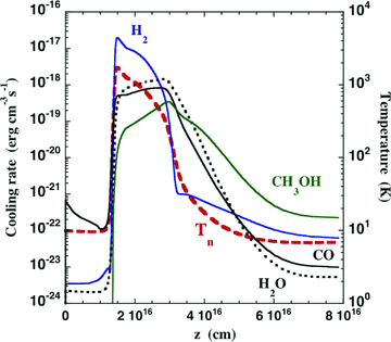
The rate of cooling by the principal molecular coolants, H2, H2O, CO and CH3OH, as computed for the reference model, a C-type shock wave of speed vs= 20 km s−1 with pre-shock density nH=n(H) + 2n(H2) = 2 × 104 cm−3. The temperature of the neutral fluid, Tn, is also plotted.
3 RESULTS AND DISCUSSION
3.1 Excitation diagram
In their study of methanol in outflow sources, Bachiller et al. (1995) made use of the ‘excitation diagram’ in order to estimate the rotational temperature from the emission-line intensities. The excitation diagram is a plot of log (Nu/gu) versus Eu/kB, where Nu is the column density, gu is the degeneracy and Eu is the excitation energy of the emitting level. In the limit of thermodynamic equilibrium, a Boltzmann distribution of emitting levels prevails, and the gradient of the curve in the excitation diagram yields the kinetic temperature of the gas.
The excitation diagram has been used extensively in the analysis of the rovibrational spectrum of H2. Owing to the fact that H2 has no permanent dipole moment, its rovibrational transitions are induced by higher order moments, principally the permanent quadrupole moment. Consequently, the radiative transition probabilities are small and the lines are optically thin, in spite of the high abundance of H2 in molecular media. Methanol, on the other hand, is a strongly dipolar molecule, and the usefulness of the excitation diagram in its case is not self-evident.
In Fig. 2 is shown, for Eu≤ 600 K, the excitation diagram for both A- and E-type methanol, as computed for our reference C-type shock wave. The diagram is broadly similar to the analogous plots for H2 in outflow sources, but there is considerable scatter around the median line. For Eu≲ 200 K, the slope of the best-fitting straight line yields a rotation temperature Trot≈ 10 K. For Eu≳ 200 K, Trot≈ 50 K. Levels with Eu≳ 200 K are populated significantly only in the hot, shocked gas. As noted by Bachiller et al. (1995), the populations of most of the energy levels are sub-thermal, and Trot≪T, the kinetic temperature.
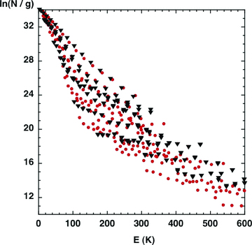
The excitation diagram of methanol (A-type: filled red circles; E-type: filled black triangles), for levels with excitation energies E≤ 600 K, as predicted by the reference model (cf. Fig. 1).
When deriving column densities from the observed methanol line intensities, Bachiller et al. (1995) assumed that the transitions were optically thin. In practice, we find that many transitions become optically thick. Although the abundance of methanol n(CH3OH) ≪ n(H2), its radiative transition probabilities are much larger than those of molecular hydrogen. The effects of the finite optical depths on the column densities deduced for some of the levels Eu≤ 100 K, considered by Bachiller et al. (1995), are considerable, as may be seen from Fig. 3. Furthermore, the assumption that all transitions are optically thin leads to the rotation temperature, deduced from the methanol lines that are observable in HIFI band 1b (Lefloch et al. 2010), being overestimated by a factor of about 3.
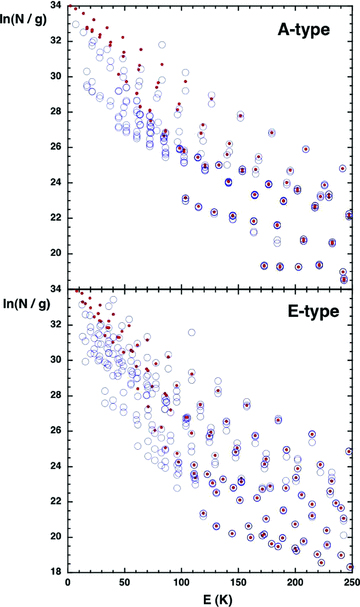
The excitation diagrams of A-type and E-type methanol, as computed for the reference model (filled red circles). Column densities, divided by the corresponding statistical weights, (2J+ 1), are plotted for levels with excitation energies E≤ 250 K. Also shown, as open blue circles, are the column densities that would be deduced on assuming that all transitions are optically thin.
Only for transitions between the lowest levels of methanol are the dipole probabilities – which are proportional to the cube of the line frequency – small enough for collisional de-excitation to become more probable than radiative decay, as the gas is compressed by the shock wave. Consequently, the relative populations of only these levels tend towards a Boltzmann distribution, as the temperature falls towards its post-shock, equilibrium value. We conclude that, for a complex and strongly dipolar molecule such as methanol, the excitation diagram is not an appropriate tool for gaining insight into the physical conditions in which the spectrum is produced.
3.2 Level populations
3.2.1 Population inversion
A number of transitions of methanol are known to mase in the interstellar medium, with the primary population inversion mechanism involving pumping either by collisions with molecular hydrogen (Class I) or by radiation (Class II). The only continuum radiation included in the present shock wave models is the 2.73-K cosmic microwave background. In outflow sources, the local radiation field is generally unknown. However, it is established that the mean energy density of the interstellar radiation field is approximately 1 eV cm−3. Dust grains absorb this radiation and re-emit in the infrared, at frequencies that are comparable with those of the methanol lines. A shock wave, on the other hand, has a dynamical energy density, ρv2s/2, which, for the models considered below, is at least 104 eV cm−3. In the absence of evidence for an enhanced infrared radiation field, we assume that dynamical processes, which heat and compress the gas and hence give rise to collisional excitation, are likely to dominate in shock waves.
In the case of the reference model, we find that the transitions A+ 70→ 61 (44.07 GHz) and E 4−1→ 30 (36.17 GHz), whose optical depths (at the line centres) attain −4.1 and −3.3, respectively, are also the most intense lines of the respective methanol types; see below. It is interesting and, we believe, significant that these transitions have been observed recently in a Class I methanol maser source, in which the emission appears to be related to an outflow along the line of sight and an associated shock wave (Voronkov et al. 2010). In addition to these intense lines, there are several weak masers, such as A− 11→ A+ 11 (0.83 GHz), whose optical depth at the line centre approaches −1. This transition – between levels which are separated by only 0.04 K – is stimulated by the cosmic background radiation field.
3.2.2 Population anti-inversion
Several transitions appear in absorption against the background radiation, notably E 20→ 3-1 (12.18 GHz), observed by Walmsley et al. (1988) to be anti-inverted towards dark clouds; in the reference model, the integrated intensity of this line is T dV=−26.2 K km s−1. In addition, the A+ 41→ 50 (57.02-GHz) and A+ 51→ 60 (6.67-GHz) transitions have TdV=−10.0 and −29.0 K km s−1, respectively. The fact that the populations of the upper and lower levels involved in these transitions should be anti-inverted is consistent with the explanation given by Walmsley et al. (1988), in connection with the 12.18-GHz line of E-type: the collisional propensities favour transitions in which K remains unchanged. As the lowest JK levels of E-type are J−1, it is possible for the 3−1 level to become overpopulated, relative to 20. In A-type, the lowest levels are J0, and hence 50 becomes overpopulated relative to 41 and 60 relative to 51. These trends are illustrated in Fig. 4, where the line intensities, T dV, are presented in the form of scatter plots, as functions of the projection quantum number of the emitting level, Kup. It may be seen that the most intense transitions of A-type emanate from levels J0 and the most intense of E-type from levels J−1, as anticipated.
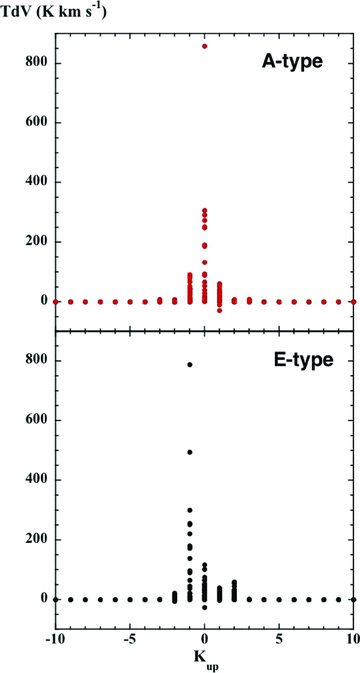
The intensities, T dV, of the lines of methanol, as predicted by the reference C-type shock model (cf. Fig. 1). The line intensities are presented in the form of scatter plots, as functions of the projection quantum number of the emitting level, Kup. Upper panel: A-type; lower panel: E-type.
3.3 Line intensities
In Fig. 5, the integrated line intensities, T dV, in units of K km s−1, are plotted against the line frequencies, ν, in GHz. The intensities were determined by integration along the direction of propagation of the shock wave, and they represent the line emission (intrinsic to the source) plus the residual cosmic background radiation (allowing for the optical depth at the frequency of the line) minus the unattenuated background; this allows for the subtraction of the radiation detected ‘off-source’ from that observed ‘on-source’ (cf. Gusdorf et al. 2008a, hereafter G08a). Thus, transitions that appear in absorption against the cosmic background have negative values of T dV.
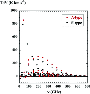
The integrated intensities, T dV, of the lines of frequency ν of A-type (filled red circles) and E-type (filled black triangles) methanol, as computed for a C-type shock wave of speed vs= 20 km s−1 with pre-shock density nH=n(H) + 2n(H2) = 2 × 104 cm−3.
The strongest emission line of A-type methanol is A+ 70→ 61 (44.07 GHz), and the strongest lines of E-type are E 4−1→ 30 (36.17 GHz) and E 5−1→ 40 (84.52 GHz). These transitions are the most intense owing to maser action, stimulated partly by the background radiation. Inversion of the populations of the upper and lower levels of these transitions is consistent with the propensity of collisions to preserve the value of K and with the fact that the ground states of A- and E-type have K= 0 and K=−1, respectively, as was mentioned above.
When the magnitude of the optical depth at the line centre ≪ 1, the line escape probability → 1 and the source function is equal to the (2.73-K) blackbody radiation intensity. Then, the subtraction of the background radiation intensity, as described above, results in T dV≈ 0. On the other hand, if the optical depth at the line centre ≫ 1, the line escape probability → 0 and the source function is equal to the blackbody radiation intensity at the rotational temperature of the line, Trot. In general, the emission is sub-thermal, as noted above, and hence Trot < Tn, the local kinetic temperature of the neutral fluid. The transitions that are prominent in Fig. 5 are the strong masers and those that appear in absorption against the cosmic background radiation. We note that the frequencies of the corresponding transitions of A- and E-type are very close: they are analogous rotational transitions within K-ladders, in which K remains constant whilst J changes.
The methanol line intensities for a small grid of C-type shock wave models are presented in Appendix A.
4 MODELS OF L1157 B1
L1157 B1, which was recently observed with the Herschel satellite (Codella et al. 2010; Lefloch et al. 2010; Nisini et al. 2010), has come to be viewed as an archetypical outflow source, associated with low-mass star formation. Although L1157 B1 appears to be a bow shock, planar C-type shock models have provided a starting point for the analysis of its spectrum (G08a; Gusdorf et al. 2008b, hereafter G08b). The shock wave may not have reached a steady state, thereby retaining J-type, in addition to C-type, characteristics; we shall refer to such shock waves as CJ-type.
The source L1157 B1 is located in the southern, blue lobe of the outflow L1157. From an analysis of Infrared Space Observatory (ISO) and other observations of H2 rovibrational transitions, SiO rotational transitions and high-J rotational transitions of CO, G08a and G08b concluded that CJ-type models reproduced best the spectrum of this source. In particular, a shock with a speed of 20 km s−1, propagating into a medium of density nH= 104 cm−3, and with an evolutionary age of 860 yr, provided an optimal fit to the observed line intensities, provided that a small fraction (approximately 10 per cent) of the elemental silicon was assumed to be initially in the form of SiO in the grain mantles. The analysis of G08a and G08b may now be extended to include the additional lines, of ortho-H2O, CO and A- and E-type methanol, which have been observed recently, by means of the Herschel satellite.
4.1 Determination of the filling factor
One issue that must be addressed when comparing radio and infrared observations of outflow sources with the predictions of shock models is the determination of the telescope beam ‘filling factor’. The diameter of the ISO beam was approximately 80 arcsec at the relevant wavelengths, whereas that of the Herschel telescope is 39 arcsec. In both cases, the beam size exceeds the angular dimensions of the source. However, the source dimensions depend to at least some degree on whether the lines are being emitted mainly by the shock-heated gas or whether the emission extends into the wake of the shock wave, where the kinetic temperature has fallen but the medium has continued to be compressed.
G08b estimated an upper limit to the filling factor in the ISO beam of 1/16 ≈ 0.06, corresponding to a 20-arcsec diameter source in the 80-arcsec beam. In the 39-arcsec Herschel beam (at the wavelengths of the HIFI band 1b), the corresponding filling factor is 0.25. More recently, Codella et al. (2010) estimated that a filling factor of 0.13 was appropriate to the methanol emission lines observed in band 1b with the HIFI instrument on board the Herschel satellite; they compared with images of this source in lower frequency methanol lines, observed with the Plateau de Bure interferometer. Given the uncertainties involved, both these determinations may be considered to be consistent with a filling factor of the order of 0.1. However, on the basis of the velocity profiles of lines of ortho-H2O and CO, observed in band 1b with HIFI, Lefloch et al. (2010) suggest that the emission may be deconvolved into that from a low-velocity component (LVC), 25 arcsec in size, and that from a high-velocity component, 7 arcsec in size. Given the beam size of 39 arcsec, the corresponding filling factors are 0.4 for the LVC and 0.03 for the HVC. Lefloch et al. tentatively identified the HVC with shock-heated gas and the LVC with the more extended wake of the shock wave.
In the calculations reported below, the integration of the line intensities was terminated at the point in the cooling flow at which the kinetic temperature of the neutral fluid had fallen to Tn= 15 K. Thus, the integration region might be understood as comprising the shock-heated gas and the shock wake. The linear size of this region is predicted to be approximately 3 × 1016 cm, corresponding to an angular size of 5 arcsec at the distance (440 ± 100 pc; Viotti 1969) of L1157. This angular size is commensurate with the dimensions of the HVC, rather than the LVC. However, the ‘real’ source is likely to be a bow shock, rather than the planar shock wave of the model, and could be more extended. Thus, it remains uncertain as to whether the filling factor of 0.03, estimated by Lefloch et al. (2010) for the HVC, or a value that is an order of magnitude larger, and appropriate to the LVC, should be applied to the models, when comparing with the observed line intensities. In practice, we consider two possible models of the source: the first is the CJ-shock model with the parameters determined by G08b and the second is a C-type model of the same shock speed (20 km s−1) but with a pre-shock gas density (nH= 2 × 104 cm−3) that is higher by a factor of 2. We shall see that a value of the filling factor at the high end of the possible range would be appropriate for the CJ-type model, whereas a value at the low end of the range would be adapted to the C-type model.
4.2 Comparison of line intensities
A comparison of line intensities in L1157 B1, observed by means of the Herschel satellite and the Caltech Submillimeter Observatory (CSO) (T dVobs), with the predictions (T dVcalc) of CJ- and C-type shock models, assuming the beam filling factors specified (see Section 4). The excitation energies of the upper levels of the transitions, Eup, are expressed relative to the ground level of the specified species; ν is the line frequency.
| Species | Transition | ν (GHz) | Eup (K) | T dVobs (K km s−1) | T dVcalca (K km s−1) | T dVcalcb (K km s−1) |
| Ortho-H2O | 110–101 | 556.936 | 27 | 12.11c | 35.86 | 4.34 |
| E-CH3OH | 112–101 | 558.344 | 168 | 0.16 | 0.04 | 0.03 |
| E-CH3OH | 3−2–2−1 | 568.566 | 32 | 0.31 | 0.26 | 0.27 |
| CO | 5–4 | 576.268 | 83 | 49.38d | 11.12 | 7.32 |
| A−-CH3OH | 22–11 | 579.085 | 45 | 0.29 | 0.13 | 0.19 |
| E-CH3OH | 12−1–11−1 | 579.151 | 178 | 0.25 | 0.47 | 0.36 |
| A+-CH3OH | 120–110 | 579.460 | 181 | 0.27 | 0.57 | 0.44 |
| A+-CH3OH | 22–11 | 579.921 | 45 | 0.21 | 0.13 | 0.20 |
| E-CH3OH | 122–112 | 580.903 | 195 | 0.09 | 0.03 | 0.02 |
| A+-CH3OH | 61–50 | 584.450 | 63 | 0.58 | 0.57 | 0.64 |
| A+-CH3OH | 73–62 | 590.278 | 115 | 0.16 | 0.08 | 0.08 |
| A−-CH3OH | 73–62 | 590.440 | 115 | 0.10 | 0.08 | 0.08 |
| E-CH3OH | 90–8−1 | 590.791 | 110 | 0.28 | 0.28 | 0.28 |
| E-CH3OH | 4−2–3−1 | 616.980 | 41 | 0.26 | 0.23 | 0.24 |
| A−-CH3OH | 32–21 | 626.626 | 52 | 0.18 | 0.12 | 0.18 |
| E-CH3OH | 13−1–12−1 | 627.170 | 209 | 0.15 | 0.25 | 0.19 |
| A+-CH3OH | 130–120 | 627.558 | 211 | 0.19 | 0.28 | 0.21 |
| A+-CH3OH | 32–21 | 629.140 | 52 | 0.24 | 0.13 | 0.19 |
| A+-CH3OH | 71–60 | 629.921 | 79 | 0.37 | 0.43 | 0.47 |
| Ortho-H2O | 212–101 | 1669.905 | 80 | 8.43e | 3.90 | 2.43 |
| CO | 3–2 | 345.796 | 33 | 43.51f | 10.54 | 4.75 |
| CO | 6–5 | 691.473 | 116 | 30.54g | 9.62 | 7.08 |
a CJ-type shock, with a beam filling factor of 0.43.
b C-type shock with a beam filling factor of 0.031.
c Sum of LVC and HVC intensities. The HVC contribution is 4.28 K km s−1 (Lefloch et al. 2010).
d Sum of LVC and HVC intensities. The HVC contribution is 3.98 K km s−1 (Lefloch et al. 2010).
e Calculated from the sum of LVC and HVC fluxes (4.2 × 10⁻²⁰ and 7.1 × 10⁻²⁰ W cm−2, respectively; Lefloch et al. 2010) in the 179-μm line, observed with PACS (Nisini et al. 2010) and smoothed to the 39-arcsec diameter HIFI band 1b beam.
f Sum of LVC and HVC intensities reported by Lefloch et al. (2010), derived from CSO observations and smoothed to the 39-arcsec diameter HIFI band 1b beam. The HVC contribution is 3.11 K km s−1.
g Sum of LVC and HVC intensities reported by Lefloch et al. (2010), derived from CSO observations and smoothed to the 39-arcsec diameter HIFI band 1b beam. The HVC contribution is 1.34 K km s−1.
Neither the CJ-type nor the C-type shock model may be deemed to provide a satisfactory fit to all of the observed line intensities. With regard to the methanol lines, the level of agreement is acceptable – and somewhat better for the C-type model – but is obtained partly by construction: the beam filling factors were determined by reference to the methanol lines, as explained above. In the cases of the 5 –4 transition of CO and the two transitions of ortho-H2O, the C-type model affords reasonable agreement with the HVC contributions to the intensities of these lines, as determined by Lefloch et al. (2010). However, the value of the beam filling factor remains the largest uncertainty in our analysis.
4.3 Comparison of line profiles
The profiles of the 557-GHz transition of ortho-H2O and the 576-GHz transition of CO, calculated for the reference C-type shock model (see Fig. 6), have strikingly similar shapes to those observed by HIFI (Lefloch et al. 2010). A similar remark applies to the 579.5- and 584.4-GHz transitions of A-type methanol, observed by Codella et al. (2010), whose profiles are also plotted in Fig. 6. We note that only the 579.5-GHz transition is optically thin, with an optical depth at the line centre τ (579.5 GHz) ≲ 0.2. The calculated line profiles imply that the emission from the cooling flow is associated with gas moving at more positive velocities, in a reverse shock. We note that the interpretation of Lefloch et al. (2010), according to which the HVC (vlsr=−7.86 km s−1) is associated with hot, shocked gas whereas the LVC (vlsr=−0.58 km s−1) is associated with the cooler wake of the shock wave, is also consistent with the emission arising in a reverse shock, propagating along the line of sight from the observer to L1157 B1.
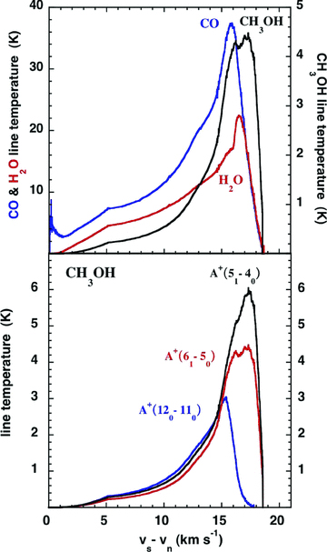
The line-temperature–velocity profiles of the 557-GHz 110–101 transition of ortho-H2O, the 576-GHz 5 –4 transition of CO, and the 579.5-GHz 120− 110 and 584.4-GHz 61–50 HIFI band 1b transitions of A+ methanol, as predicted by the reference C-type shock model (cf. Fig. 1). The lower frequency 538.6-GHz 51–40 A+ transition is also plotted, for comparison.
5 CONCLUDING REMARKS
We have computed the intensities of the lines of methanol that are expected to be emitted by shock waves in molecular outflows. The results of very recent calculations of the rate coefficients for the excitation of methanol in collisions with ortho- and para-H2 and with He were incorporated in the shock wave model. Line intensities are provided for a small grid of C-type shock waves, which is intended to guide the interpretation of Herschel and other observations of outflow sources.
We find that the most intense transitions are masers, with the population inversion being induced by collisions, principally with molecular hydrogen. Observations of two of these transitions2 have been reported recently in a Class I methanol maser source, G309.39 −0.14, which is associated with a probable molecular outflow (Voronkov et al. 2010). The same collisional propensities that lead to maser emission result in other transitions appearing in absorption against the cosmic background radiation, owing to population anti-inversion, as originally postulated by Walmsley et al. (1988).
A simulation of Herschel observations of methanol in the outflow source L1157 B1 was undertaken, with limited success. No single shock wave model provides a satisfactory fit to these observations, partly because of the considerable uncertainty in the value that should be adopted for the beam filling factor. Whilst ground-based interferometric observations of lower frequency methanol transitions provide some indication of the angular size of the source, the high-frequency lines, observed with Herschel, may arise in shock-heated gas, of smaller angular dimensions. Further observations of outflow sources, using the Herschel satellite and other observing facilities, may help to resolve this issue.
The numerical value, n(CH3OH*)/nH= 1.86 × 10⁻⁵, of the initial fractional abundance of methanol ice was deduced from the observations by Gibb et al. (2000), of the ice mantle composition in W33A, together with the fractional abundance of gas-phase carbon in ζ Oph, nC/nH= 1.38 × 10⁻⁴ (Savage & Sembach 1996), assuming that carbon in the gas phase is predominantly in the form of CO and that the initial gas-to-solid phase abundance ratio n(CO)/n(CO*) = 10.
A+ 70→ 61 (44.07 GHz) and E 4−1→ 30 (36.17 GHz).
This work was supported partially by a research grant from the STFC (UK).
REFERENCES
Appendix
APPENDIX A: PREDICTED METHANOL LINE INTENSITIES

A sample of A-type CH3OH line intensities, T dV K km s−1, for a grid of C-type shock models, identified by the shock speed, in km s−1, and the pre-shock density, in cm−3 [e.g. v10n2e4 signifies vs= 10 km s−1 and nH=n(H) + 2n(H2) = 2 × 104 cm−3]. The upper and lower levels of the transition are identified by the values of J, the rotational quantum number, and K, the projection of the rotational angular momentum on the methanol symmetry axis. States A+ and A− are distinguished by positive or negative values of K. Eup is the excitation energy of the upper level and ν is the frequency of the transition. Note that the level energies derive from theoretical calculations and hence the corresponding line frequencies are not of spectroscopic accuracy (see Section 2.1). The discrepancies with the empirical line frequencies increase as the frequencies decrease and become small differences between relatively large numbers. The complete table is available as online Supporting Information.
| Jup | Kup | Jlow | Klow | Eup (K) | ν (GHz) | v10n2e4 | v15n2e4 | v20n2e4 | v30n2e4 | v40n2e4 |
| 1 | 1 | 0 | 0 | 16.810 | 350.32 | 0.010 940 | 2.7718 | 27.631 | 36.491 | 43.363 |
| 1 | 1 | 2 | 0 | 16.810 | 206.42 | 0.000 113 04 | 1.4431 | 17.935 | 23.302 | 28.354 |
| 1 | 0 | 0 | 0 | 2.3000 | 47.970 | 0.031 933 | 6.2146 | 66.701 | 68.904 | 64.716 |
| 1 | −1 | 1 | 1 | 16.850 | 0.820 00 | 5.5816e−05 | 0.259 23 | 6.6151 | 5.9317 | 5.3781 |
| 1 | −1 | 1 | 0 | 16.850 | 303.17 | 0.012 626 | 3.4114 | 32.800 | 42.954 | 50.736 |
As Table A1 but for nH=n(H) + 2n(H2) = 2 × 105 cm−3. The complete table is available as online Supporting Information.
| Jup | Kup | Jlow | Klow | Eup (K) | ν (GHz) | v10n2e5 | v15n2e5 | v20n2e5 | v30n2e5 | v40n2e5 |
| 1 | 1 | 0 | 0 | 16.810 | 350.32 | 0.107 20 | 15.390 | 87.332 | 100.55 | 123.88 |
| 1 | 1 | 2 | 0 | 16.810 | 206.42 | 0.029 206 | 9.6122 | 56.740 | 62.127 | 76.548 |
| 1 | 0 | 0 | 0 | 2.3000 | 47.970 | 0.043 704 | 7.5725 | 44.989 | 44.350 | 47.599 |
| 1 | −1 | 1 | 1 | 16.850 | 0.820 00 | −7.6602e−05 | 0.333 62 | 3.3947 | 2.9679 | 3.1051 |
| 1 | −1 | 1 | 0 | 16.850 | 303.17 | 0.132 34 | 18.117 | 100.72 | 116.82 | 143.00 |
A sample of E-type CH3OH line intensities, T dV K km s−1, for a grid of C-type shock models, identified by the shock speed, in km s−1, and the pre-shock density, in cm−3 [e.g. v10n2e4 signifies vs= 10 km s−1 and nH=n(H) + 2n(H2) = 2 × 104 cm−3]. The upper and lower levels of the transition are identified by the values of J, the rotational quantum number, and K, the projection of the rotational angular momentum on the methanol symmetry axis. Eup is the excitation energy of the upper level and ν is the frequency of the transition. Note that the level energies derive from theoretical calculations, and hence the corresponding line frequencies are not of spectroscopic accuracy (see Section 2.1). The discrepancies with the empirical line frequencies increase as the frequencies decrease and become small differences between relatively large numbers. The complete table is available as online Supporting Information.
| Jup | Kup | Jlow | Klow | Eup (K) | ν (GHz) | v10n2e4 | v15n2e4 | v20n2e4 | v30n2e4 | v40n2e4 |
| 0 | 0 | 1 | −1 | 13.110 | 108.60 | 0.018 654 | 3.6723 | 26.672 | 30.775 | 33.350 |
| 1 | 0 | 0 | 0 | 15.410 | 47.970 | 0.006 3220 | 2.3454 | 32.981 | 34.315 | 33.974 |
| 1 | 0 | 1 | −1 | 15.410 | 156.57 | 0.038 433 | 6.2616 | 44.573 | 53.728 | 57.837 |
| 1 | 0 | 2 | −1 | 15.410 | 60.640 | −0.000 704 71 | 0.859 84 | 5.4410 | 3.7457 | 5.7919 |
| 1 | 1 | 0 | 0 | 23.360 | 213.53 | 0.008 9894 | 2.6696 | 25.974 | 31.583 | 35.547 |
As Table A3 but for nH=n(H) + 2n(H2) = 2 × 105 cm−3. The complete table is available as online Supporting Information.
| Jup | Kup | Jlow | Klow | Eup (K) | ν (GHz) | v10n2e5 | v15n2e5 | v20n2e5 | v30n2e5 | v40n2e5 |
| 0 | 0 | 1 | −1 | 13.110 | 108.60 | 0.045 916 | 7.7844 | 41.307 | 43.175 | 50.953 |
| 1 | 0 | 0 | 0 | 15.410 | 47.970 | 0.014 560 | 4.3532 | 32.395 | 32.040 | 36.100 |
| 1 | 0 | 1 | −1 | 15.410 | 156.57 | 0.091 796 | 12.293 | 62.782 | 65.820 | 75.922 |
| 1 | 0 | 2 | −1 | 15.410 | 60.640 | 0.027 512 | 5.1618 | 26.238 | 28.389 | 34.948 |
| 1 | 1 | 0 | 0 | 23.360 | 213.53 | 0.039 368 | 9.0531 | 52.661 | 56.486 | 69.275 |
SUPPORTING INFORMATION
Additional Supporting Information may be found in the online version of this article:
Section 2.1. The computed level energies and A values.
Please note: Blackwell Publishing are not responsible for the content or functionality of any supplementary materials supplied by the authors. Any queries (other than missing material) should be directed to the corresponding author for the article.
