


Abstract
We report the detection of a magnetic field on the Of?p star HD 108. Spectropolarimetric observations conducted in 2007, 2008 and 2009, respectively, with NARVAL@Télescope Bernard Lyot (TBL) and Echelle SpectroPolarimetric Device for the Observation of Stars at Canada–France–Hawaii Telescope (ESPaDOnS@CFHT) reveal a clear Zeeman signature in the average Stokes V profile, stable on time-scales of days to months and slowly increasing in amplitude on time-scales of years. We speculate that this time-scale is the same as that on which Hα emission is varying and is equal to the rotation period of the star. The corresponding longitudinal magnetic field, measured during each of the three seasons, increases slowly from 100 to 150 G, implying that the polar strength of the putatively dipolar large-scale magnetic field of HD 108 is at least 0.5 kG and most likely of the order of 1–2 kG.
The stellar and wind properties are derived through a quantitative spectroscopic analysis with the code cmfgen. The effective temperature is difficult to constrain because of the unusually strong He i λλ4471, 5876 lines. Values in the range of 33 000–37 000 K are preferred. A mass-loss rate of about 10−7 M⊙ yr−1 (with a clumping factor f= 0.01) and a wind terminal velocity of 2000 km s−1 are derived. The wind confinement parameter η★ is larger than 100, implying that the wind of HD 108 is magnetically confined.
Stochastic short-term variability is observed in the wind-sensitive lines but not in the photospheric lines, excluding the presence of pulsations. Material infall in the confined wind is the most likely origin for lines formed in the inner wind. Wind clumping also probably causes part of the Hα variability. The projected rotational velocity of HD 108 is lower than 50 km s−1, consistent with the spectroscopic and photometric variation time-scales of a few decades. Overall, HD 108 is very similar to the magnetic O star HD 191612 except for an even slower rotation.
1 INTRODUCTION
Very little is known about magnetic fields of O stars and very few O stars are yet known as magnetic; preliminary results (e.g. Donati et al. 2002, 2006; Bouret et al. 2008; Petit et al. 2008) suggest that most magnetic O stars could be the high-mass equivalent of magnetic chemically peculiar A and B stars (the so-called Ap and Bp stars) with fields of primordial origin, i.e. fossil remnants from the formation stage (Donati & Landstreet 2009). They are also suspected to be progenitors of highly magnetic neutron stars and magnetars (e.g. Ferrario & Wickramasinghe 2008; Petit et al. 2008), although alternative explanations exist (Davies et al. 2009).
Whenever known, rotation rates of magnetic O stars are significantly smaller than non-magnetic O stars of similar spectral types, further strengthening the analogy with the lower mass Ap and Bp stars. Evolutionary models of massive stars including magnetic fields also suggest that the internal rotation is strongly affected by the presence of magnetic fields, enforcing in particular mostly solid-body rotation profiles throughout the bulk of the outer radiative zone (Maeder & Meynet 2003, 2004). Last but not least, magnetic fields are potentially capable of affecting the powerful radiative winds of O stars (Babel & Montmerle 1997) and, in some extreme cases, of fully dissipating their angular momentum through wind magnetic braking (ud-Doula, Owocki & Townsend 2009). Lives of magnetic O stars are therefore expected to differ significantly from those of their non-magnetic counterparts.
In this respect, the prototypical cases of θ1 Ori C (Donati et al. 2002) and HD 191612 (Donati et al. 2006) are very interesting. The magnetic field of θ1 Ori C (about 1.1 kG tilted at about 45° to the rotation axis) is strong enough to deflect the wind flows from both magnetic hemispheres towards the magnetic equator where they collide, generating a strong shock, a very hot (coronal-like) post-shock region and a denser cooling disc (more or less confined to the magnetic equatorial plane). Emission in Balmer lines exhibits very strong rotational modulation, the amount of emission being directly related to the geometry of the cooling disc as seen from the Earth: strongest when the disc is seen pole-on and weakest when the disc is seen edge-on (e.g. Donati et al. 2002). The presence of magnetic fields and the very similar Hα modulation reported for HD 191612 suggests that this star is analogous to θ1 Ori C (Donati et al. 2006), but more evolved and much more slowly rotating (538 d versus 15.4 d for θ1 Ori C) as a likely result of wind magnetic braking. Recent (yet unpublished) data (Wade et al., in preparation) fully confirm the initial conclusions and the remarkable similarity between HD 191612 and θ1 Ori C.
Exploring further the potential impact of magnetic fields on the life of massive stars requires new magnetic O stars to be identified. From the example of θ1 Ori C and HD 191612, those exhibiting periodically varying Hα emission are likely to be very good candidates. In particular, HD 108 is interesting. It is a member of the Of?p class composed of the Galactic stars HD 191612, HD 148937, NGC 1624-2 and CPD −28°2561, the latter two recently discovered by Walborn et al. (2010). This class is principally defined by emission in the C iii 4647–4650 lines at least as strong as in the neighbouring N iii 4630–4640 lines. Secondary classification criteria include sharp emission or P Cygni profiles in He i and Balmer lines. As θ1 Ori C and HD 191612, HD 108 shows spectral-type variations (from 04 to 08) due to changes in the strength of its He i lines. They (and the Balmer lines too) fluctuate between pure absorption and P Cygni profiles. These line morphologies define ‘low’ and ‘high’ states, respectively. The changes are correlated with photometric variations: HD 108 is brighter when the emission components are stronger, again similar to HD 191612. They seem to occur with a period of a few decades (Nazé, Vreux & Rauw 2001; Barannikov 2007) compared to 538 d for HD 191612 (Walborn et al. 2004; Howarth et al. 2007). If the analogy with θ1 Ori C and HD 191612 holds, HD 108 could thus potentially show up as a rather extreme case of wind magnetic braking. Note that a marginal detection based on a single exposure was reported by Hubrig et al. (2008) for the third member of the Galactic Of?p class, HD 148937 [but see Silvester et al. (2009) for a discussion of the significance of the detection]. Further observations are required to confirm this detection.
To investigate this issue, we initiated a spectropolarimetric monitoring programme of HD 108 using NARVAL at the 2-m Télescope Bernard Lyot (TBL) in the French Pyrenees and later on Echelle SpectroPolarimetric Device for the Observation of Stars (ESPaDOnS) at the 3.6-m Canada–France–Hawaii Telescope (CFHT) atop Mauna Kea, Hawaii.1 Reports indicate that HD 108 has just passed the epoch of minimum Hα emission (Nazé et al., in preparation), suggesting that longitudinal magnetic fields are also close to their minimum value and slowly rising again (provided the analogy with θ1 Ori C and HD 191612 holds).
We report here the first results after three observing seasons (2007–2009). In particular, we report the detection of a longitudinal magnetic field of about 100 G at the surface of HD 108, suggesting that the analogy with θ1 Ori C and HD 191612 is likely. We also carry out a detailed spectral analysis to obtain updated constraints on the parameters of HD 108. We finally discuss briefly the implications of our results for understanding how magnetic fields affect the lives of massive stars.
2 OBSERVATIONS
Spectropolarimetric observations of HD 108 were collected with NARVAL@TBL and ESPaDOnS@CFHT in 2007 October, 2008 October and 2009 July–October. Altogether, 110 sequences (24 in 2007, 27 in 2008 and 59 in 2009) were obtained in multiple runs, each sequence consisting of four individual subexposures taken in different polarimeter configurations.
From each set of four subexposures we derive a mean Stokes V spectrum following the procedure of Donati et al. (1997), ensuring in particular that all spurious signatures are removed at first order. Null polarization spectra (labelled N) are calculated by combining the four subexposures in such a way that polarization cancels out, allowing us to check that no spurious signals are present in the data (see Donati et al. 1997, for more details on how N is defined). All frames were processed using libre ESpRIT (Donati et al. 1997), a fully automatic reduction package installed at TBL and CFHT for optimal extraction of NARVAL and ESPaDOnS spectra. The peak signal-to-noise ratios (S/N) per 2.6 km s−1 velocity bin range from 140 to 1100, depending on the instrument, on the exposure time and on weather conditions (see Table 1 for a complete log).
Journal of observations.
| Date | Instrument | HJD (2454 000+) | ut (h:m:s) | texp (s) | S/N | σLSD (10−4Ic) | Bz (G) |
| 2007 Oct 15 | NARVAL | 389.389 26–389.477 36 | 21:14:22–23:21:14 | 3 × 4 × 900 | 500–590 | 2.2 | −94.2±54.3 |
| 2007 Oct 16/17 | NARVAL | 390.485 64–390.573 75 | 23:33:12–01:40:05 | 3 × 4 × 900 | 350–550 | 2.6 | −51.3±63.8 |
| 2007 Oct 18 | NARVAL | 392.331 25–392.419 36 | 19:50:58–21:57:51 | 3 × 4 × 900 | 340–390 | 3.3 | 0.9±82.9 |
| 2007 Oct 19 | NARVAL | 393.363 08–393.451 20 | 20:36:51–22:43:45 | 3 × 4 × 900 | 580–620 | 2.1 | −66.6±50.4 |
| 2007 Oct 20 | NARVAL | 394.345 87–394.433 99 | 20:12:07–22:19:01 | 3 × 4 × 900 | 560–600 | 2.1 | −99.6±50.8 |
| 2007 Oct 21 | NARVAL | 395.373 85–395.461 97 | 20:52:28–22:59:21 | 3 × 4 × 900 | 560–590 | 2.1 | −215.1±52.0 |
| 2007 Oct 23 | NARVAL | 397.351 03–397.439 15 | 20:19:43–22:26:37 | 3 × 4 × 900 | 540–590 | 2.1 | −70.6±52.7 |
| 2007 Oct 24 | NARVAL | 398.352 62–398.440 76 | 20:22:03–22:28:59 | 3 × 4 × 900 | 550–600 | 2.2 | −25.6±52.9 |
| 2008 Oct 14 | NARVAL | 754.309 40–754.485 59 | 19:19:21–23:33:04 | 5 × 4 × 900 | 530–610 | 1.6 | −81.0±39.2 |
| 2008 Oct 16 | ESPaDOnS | 755.857 07–755.889 27 | 08:28:03–09:14:25 | 2 × 4 × 650 | 540–580 | 2.7 | −115.4±69.5 |
| 2008 Oct 23 | NARVAL | 763.290 85–763.467 08 | 18:53:06–23:06:53 | 5 × 4 × 900 | 460–550 | 1.9 | −137.0±48.0 |
| 2008 Oct 24 | NARVAL | 764.271 21–764.447 46 | 18:24:52–22:38:41 | 5 × 4 × 900 | 600–650 | 1.5 | −106.9±37.9 |
| 2008 Oct 25 | NARVAL | 765.282 97–765.459 22 | 18:41:52–22:55:41 | 5 × 4 × 900 | 420–520 | 2.0 | −56.4±51.7 |
| 2008 Oct 26 | NARVAL | 766.269 93–766.446 19 | 18:23:09–22:36:59 | 5 × 4 × 900 | 420–530 | 1.9 | −66.5±50.3 |
| 2009 Jul 05 | ESPaDOnS | 1018.043 24–1018.105 93 | 13:00:46–14:31:02 | 2 × 4 × 1300 | 950–1040 | 1.6 | −134.4±43.8 |
| 2009 Jul 07 | ESPaDOnS | 1020.040 33–1020.104 16 | 12:56:22–14:28:16 | 2 × 4 × 1300 | 830–950 | 1.7 | −286.0±47.3 |
| 2009 Jul 09 | ESPaDOnS | 1022.043 07–1022.105 52 | 13:00:05–14:30:00 | 2 × 4 × 1300 | 1070–1090 | 1.5 | −222.3±40.1 |
| 2009 Jul 13 | ESPaDOnS | 1026.038 27–1026.101 62 | 12:52:44–14:23:58 | 2 × 4 × 1300 | 1030–1060 | 1.5 | −140.0±40.6 |
| 2009 Jul 14 | ESPaDOnS | 1027.051 50–1027.114 23 | 13:11:41–14:42:01 | 2 × 4 × 1300 | 1100–1110 | 1.4 | −142.9±39.8 |
| 2009 Jul 21 | NARVAL | 1033.538 71–1033.635 38 | 00:52:37–03:11:49 | 3 × 4 × 750 | 330–520 | 2.7 | −130.7±66.4 |
| 2009 Jul 25 | NARVAL | 1037.531 56–1037.605 79 | 00:41:56–02:28:49 | 3 × 4 × 750 | 480–510 | 2.5 | −160.0±62.2 |
| 2009 Jul 26 | NARVAL | 1038.577 50–1038.647 09 | 01:47:60–03:28:11 | 3 × 4 × 700 | 330–450 | 3.1 | 121.0±82.4 |
| 2009 Jul 27 | NARVAL | 1039.539 64–1039.658 75 | 00:53:23–03:44:53 | 4 × 4 × 806 | 310–440 | 2.7 | −28.1±74.0 |
| 2009 Jul 28 | NARVAL | 1040.538 24–1040.626 33 | 00:51:16–02:58:06 | 3 × 4 × 900 | 260–460 | 3.2 | −113.0±87.6 |
| 2009 Jul 29 | NARVAL | 1041.530 43–1041.618 52 | 00:39:56–02:46:46 | 3 × 4 × 900 | 510–580 | 2.2 | −27.8±55.3 |
| 2009 Jul 30 | NARVAL | 1042.541 92–1042.630 03 | 00:56:23–03:03:16 | 3 × 4 × 900 | 580–640 | 2.0 | −62.7±50.7 |
| 2009 Jul 31 | NARVAL | 1043.523 99–1043.643 94 | 00:30:28–03:23:11 | 4 × 4 × 812 | 500–550 | 2.0 | −161.6±51.3 |
| 2009 Aug 01 | NARVAL | 1044.541 74–1044.624 18 | 00:55:57–02:54:39 | 3 × 4 × 812 | 540–590 | 2.1 | −38.0±55.1 |
| 2009 Aug 02 | NARVAL | 1045.537 83–1045.626 15 | 00:50:14–02:57:24 | 3 × 4 × 900 | 390–420 | 3.1 | −99.4±80.0 |
| 2009 Aug 04 | NARVAL | 1047.561 89–1047.649 99 | 01:24:42–03:31:34 | 3 × 4 × 900 | 560–600 | 2.1 | −161.4±36.6 |
| 2009 Aug 05 | NARVAL | 1048.518 90–1048.607 01 | 00:22:43–02:29:35 | 3 × 4 × 900 | 580–600 | 2.1 | −141.9±52.7 |
| 2009 Sep 03 | ESPaDOnS | 1078.074 57 | 13:41:03 | 4 × 1300 | 940 | 2.2 | −109.7±55.8 |
| 2009 Sep 08 | ESPaDOnS | 1082.950 60–1083.013 00 | 10:42:24–12:12:14 | 2 × 4 × 1300 | 1030–1040 | 1.5 | −156.1±38.2 |
| 2009 Sep 25 | ESPaDOnS | 1099.882 04–1099.946 11 | 09:03:29–10:35:43 | 2 × 4 × 1300 | 990–1010 | 1.5 | −208.5±40.3 |
| 2009 Oct 01 | ESPaDOnS | 1105.862 47–1105.925 25 | 08:35:21–10:05:45 | 2 × 4 × 1300 | 880–960 | 1.7 | −140.4±45.2 |
| 2009 Oct 05 | ESPaDOnS | 1109.962 49–1110.025 67 | 10:59:28–12:30:27 | 2 × 4 × 1300 | 140–600 | 3.2 | −273.8±84.1 |
| 2009 Oct 10 | ESPaDOnS | 1114.873 31–1114.937 01 | 08:51:12–10:22:56 | 2 × 4 × 1300 | 1060–1100 | 1.6 | −239.7±41.2 |
Note. Columns 1–6 list the date, the instrument used, the range of heliocentric Julian dates, the range of ut times, the number of sequences and the exposure time per individual sequence subexposure, and the range of peak S/N (per 2.6 km s−1 velocity bin), for each night of observation. Column 7 lists the rms noise level (relative to the unpolarized continuum level and per 7.2 km s−1 velocity bin) in the circular polarization profile produced by LSD once averaged over the whole night. Column 8 gives the longitudinal field strength (and the corresponding 1σ error bar) determined from the night-averaged polarization spectrum.
3 MAGNETIC DETECTION
Least-squares deconvolution (LSD; Donati et al. 1997) was applied to all observations. The line list was constructed manually to include the few moderate to strong absorption lines that are no more than moderately affected by the wind. All lines showing strong emission from the wind and/or circumstellar environment at the time of our observations (e.g. Hα) were excluded from the list. The remaining very weak contamination is not circularly polarized. Hence, it only slightly affects the calculation of the longitudinal field but not the Stokes V profile and thus the field detection. The C iv lines at 5801.3 and 5812.0 Å are used as reference photospheric lines from which we obtain the average radial velocity of HD 108 (about −62 km s−1); about a handful of unblended absorption lines that are not blueshifted with respect to the reference frame by more than 30 km s−1 are also included in the list. We ended up with a list of 16 lines, whose characteristics are summarized in Table 2. All LSD profiles were produced on a spectral grid with a velocity bin of 7.2 km s−1, providing reasonable sampling given the significant macroturbulent broadening detected on HD 108 (see Section 4.3).
Lines used for LSD. The line depths (Column 3) were directly measured from our spectra while the Landé factors (Column 4) were derived assuming LS coupling. Boldface indicates lines with the weakest wind contamination.
| Wavelength (Å) | Element | Depth (Ic) | Landé factor |
| 4026.198 | He i | 0.33 | 1.1 |
| 4199.839 | He ii | 0.15 | 1.0 |
| 4379.201 | N iii | 0.06 | 1.1 |
| 4387.929 | He i | 0.08 | 1.0 |
| 4471.483 | He i | 0.41 | 1.1 |
| 4510.963 | N iii | 0.06 | 1.1 |
| 4514.854 | N iii | 0.08 | 1.2 |
| 4541.593 | He ii | 0.20 | 1.0 |
| 4713.139 | He i | 0.13 | 1.5 |
| 4921.931 | He i | 0.14 | 1.0 |
| 5015.678 | He i | 0.11 | 1.0 |
| 5411.516 | He ii | 0.25 | 1.0 |
| 5592.252 | O iii | 0.40 | 1.0 |
| 5801.313 | C iv | 0.20 | 1.2 |
| 5811.970 | C iv | 0.15 | 1.3 |
| 7065.176 | He i | 0.22 | 1.5 |
Using this line list, we obtained, for all collected spectra, mean circular polarization (LSD Stokes V), mean polarization check (LSD N) and mean unpolarized (LSD Stokes I) profiles (corresponding to a weighted – relative to S/N2, line depth and wavelength – average line of a central wavelength of 5500 Å and Landé factor of 1.2). Averaging together all LSD profiles recorded on each night of observation (with weights proportional to the inverse variance of each profile) yields relative noise levels ranging from 1.4 to 3.3 (in units of 10−4Ic) in V and N profiles. In general, no significant magnetic signature was detected in individual spectra. In a few exceptional cases, however, nightly averages of spectra showed marginal evidence for the presence of magnetic fields at the surface of HD 108 (see Column 8 of Table 1).
Using a line list containing the five lines with weakest interstellar contamination and smallest blueshifts with respect to the stellar rest velocity (indicated in boldface in Table 2), the detected Zeeman signature is compatible (within the noise level) with that derived using the full line list, confirming that the detected signature is due to magnetic fields at the surface of the star.
The detected Zeeman signature (featuring a peak-to-peak amplitude of 0.04 per cent) cannot be attributed to the small cross-talk between circular and linear polarizations that ESPaDOnS and NARVAL used to suffer (smaller than 1 per cent on ESPaDOnS during our 2009 run and smaller than 4 per cent for NARVAL and for ESPaDOnS at all other epochs) as this would imply that photospheric lines of HD 108 exhibit roughly antisymmetric linear polarization signatures with peak-to-peak amplitudes of at least 1–4 per cent – a highly unlikely possibility. It would also imply that the Zeeman signature detected with ESPaDOnS in 2009 is smaller (by at least a factor of 4) than those measured with NARVAL and ESPaDOnS at all other epochs, reflecting the instrumental fix implemented on ESPaDOnS in early 2009; since this is not the case, we can safely claim that the detected Zeeman signature is not caused by a cross-talk problem.
For each of the main observing seasons (2007, 2008 and 2009), we constructed average LSD signatures and corresponding variances. In 2009, the mean Stokes V signature is clearly detected with a reduced chi-squared χ2r within the line profile of about 132 (see Fig. 1); in 2008 and 2007, the corresponding χ2r values (2.5 and 1.5, respectively) are smaller but large enough to claim a definite detection in 2008 and a marginal one in 2007 (with a 98 per cent confidence level). No signal is detected in the N (polarization check) profile, demonstrating that the signal we detect is truly attributable to circular polarization. The variance profiles show no evidence for variability of the Zeeman signatures throughout each season, even in 2009 where the S/N is highest. We therefore conclude that the Zeeman signature, if varying, is changing very slowly on typical time-scales of years rather than months or weeks. The longitudinal fields we measure in 2007, 2008 and 2009 [using the first-order moment method of Donati et al. (1997)– inspired by Semel (1967)– and integrating through a velocity range from −300 to 120 km s−1] are, respectively, equal to −90 ± 20, −100 ± 20 and −150 ± 10 G (1σ error bars), suggesting a slow rise in field strength on time-scales of years.

LSD circularly polarized (Stokes V), polarization check (N) and unpolarized (Stokes I) profiles of HD 108 (top, middle, bottom curves, respectively) averaged over all NARVAL and ESPaDOnS data collected in 2009. LSD V and N profiles are expanded by a factor of 250 and shifted upwards (by 1.15 and 1.05) for display purposes.
Both the detection of a magnetic field on HD 108 and the lower limit of months to years on the time-scale on which the Zeeman signatures are varying strengthen the aforementioned analogy with θ1 Ori C and HD 191612. For these stars, the longitudinal fields and line emissions (and photometric brightness for HD 191612) are all modulated with the same period (the rotation period). We thus speculate that the longitudinal field of HD 108 tightly correlates with line emission and photospheric brightness, weakest at minimum emission and minimum brightness and strongest at maximum emission and maximum brightness (as in HD 191612). This is in agreement with the slow increase in both longitudinal field and Balmer line emission that we observe from 2007 to 2009.
If we assume that the magnetic field at the surface of HD 108 is grossly dipolar (e.g. like that of θ1 Ori C and HD 191612; Donati et al. 2002, 2006), it implies that the polar field at the surface of the star (roughly four times larger than the maximum longitudinal field; e.g. Donati et al. 2002) is at least 0.5–0.6 kG. This estimate is based on the classical relation between longitudinal and polar fields of Preston (1967) (see also Donati & Landstreet 2009). If we further take into account that HD 108 is still at least 10 yr away from longitudinal field maximum (e.g. given the observed photometric variations; Barannikov 2007), we conclude that the polar field of HD 108 is likely stronger than 1 kG and potentially as strong as (or even stronger than) that of HD 191612.
4 STELLAR AND WIND PHYSICAL PROPERTIES
Nazé, Walborn & Martins (2008) conducted a study of the ‘high’ optical state of HD 108. Here, we present a new analysis based on our NARVAL spectra collected in 2008 and 2009, as well as Far Ultraviolet Spectroscopic Explorer (FUSE) data obtained in 2007 and 2008 and retrieved from the MAST archive. These data correspond to the ‘low’ state of HD108. The spectral analysis was performed using the atmosphere code cmfgen (Hillier & Miller 1998).
An exhaustive description of the atmosphere models can be found in Hillier & Miller (1998). In practice, an iterative scheme is developed. At each step, the radiative transfer equation is solved in spherical geometry. With the resulting specific intensity, the rate equations yield non-local thermodynamic equilibrium level populations which in turn are used to compute opacities. These opacities are subsequently injected in the radiative transfer equation in the next iteration step. The temperature structure results from the radiative equilibrium equation. Line blanketing is included by means of the super-level approach. The atmosphere velocity structure is given as input and results from the connection of a pseudo-hydrostatic structure (taken from TLUSTY models; Lanz & Hubeny 2003) with a so-called β-velocity law representing the wind structure (e.g. Lamers & Cassinelli 1999). The density structure directly follows from mass conservation. All models take into account clumping and Auger ionization by X-rays (using the X-ray luminosity of Nazé et al. 2004). We adopt a solar chemical composition (Grevesse, Asplund & Sauval 2007) except for helium and nitrogen (see below). Once the model atmosphere is obtained, a formal solution to the radiative transfer equation is performed to produce the final synthetic spectra.
The derived stellar and wind properties of HD 108 are gathered in Table 3. The results of Nazé et al. (2008) are also given for comparison.
Summary of stellar and wind properties of HD 108.
| Present work | Nazé et al. 2008 | |
| Teff (K) | 35 000 ± 2000 | 37 000 ± 2000 |
| log g (cgs) | 3.50 ± 0.20 | 3.75 ± 0.10 |
| log L★/L⊙ | 5.70 ± 0.10 | 5.40 ± 0.10 |
| R★/R⊙ | 19.2+3.3−2.8 | 12.3 ± 2.1 |
| M★/M⊙ | 43+32−18 | ∼35 |
| v sin i (km s−1) | <50 | ∼40 |
log  | −7.0+0.20−0.40 | −6.5/−7.0 |
| v∞ (km s−1) | 2000 ± 300 | 2000 |
| vcl (clumping; km s−1) | 30 | 30 |
| f (clumping) | 0.01 | 0.01 |
| E(B−V) | 0.47 | – |
| log LX/LBOL | −6.2 | – |
| He/H (by number) | 3.0 × 10⁻¹ | 0.1a |
| N/H (by number) | 3.6 × 10⁻⁴ | – |
| Present work | Nazé et al. 2008 | |
| Teff (K) | 35 000 ± 2000 | 37 000 ± 2000 |
| log g (cgs) | 3.50 ± 0.20 | 3.75 ± 0.10 |
| log L★/L⊙ | 5.70 ± 0.10 | 5.40 ± 0.10 |
| R★/R⊙ | 19.2+3.3−2.8 | 12.3 ± 2.1 |
| M★/M⊙ | 43+32−18 | ∼35 |
| v sin i (km s−1) | <50 | ∼40 |
| log | −7.0+0.20−0.40 | −6.5/−7.0 |
| v∞ (km s−1) | 2000 ± 300 | 2000 |
| vcl (clumping; km s−1) | 30 | 30 |
| f (clumping) | 0.01 | 0.01 |
| E(B−V) | 0.47 | – |
| log LX/LBOL | −6.2 | – |
| He/H (by number) | 3.0 × 10⁻¹ | 0.1a |
| N/H (by number) | 3.6 × 10⁻⁴ | – |
a Adopted.
Summary of stellar and wind properties of HD 108.
| Present work | Nazé et al. 2008 | |
| Teff (K) | 35 000 ± 2000 | 37 000 ± 2000 |
| log g (cgs) | 3.50 ± 0.20 | 3.75 ± 0.10 |
| log L★/L⊙ | 5.70 ± 0.10 | 5.40 ± 0.10 |
| R★/R⊙ | 19.2+3.3−2.8 | 12.3 ± 2.1 |
| M★/M⊙ | 43+32−18 | ∼35 |
| v sin i (km s−1) | <50 | ∼40 |
| log | −7.0+0.20−0.40 | −6.5/−7.0 |
| v∞ (km s−1) | 2000 ± 300 | 2000 |
| vcl (clumping; km s−1) | 30 | 30 |
| f (clumping) | 0.01 | 0.01 |
| E(B−V) | 0.47 | – |
| log LX/LBOL | −6.2 | – |
| He/H (by number) | 3.0 × 10⁻¹ | 0.1a |
| N/H (by number) | 3.6 × 10⁻⁴ | – |
a Adopted.
4.1 Photospheric parameters
The effective temperature Teff is usually derived from the relative strength of He i to He ii lines in O stars. In the case of HD 108, however, this procedure turned out to be considerably more complex. First, some He i lines present a central emission component the origin of which is not known (e.g. He i λλ4144, 4388, 4920). Secondly, most lines have highly asymmetric profiles, their blue wing rising towards the continuum less steeply than their red wings (see e.g. Fig. 1). Thirdly, He iλ5876 and, more worrisome, the normally well-behaved He iλ4471 line show unusually strong absorption in the 2007–2009 spectra. In fact, these two lines are the strongest features of the entire optical spectrum. Fig. 2 illustrates the problems encountered when fitting the He i lines. It shows the difference between the observed He i equivalent widths and those of various models. Clearly, He i λλ4471, 5876 are always too weak in our models, because both the line depth and equivalent width are weaker than observed. The situation is improved only for very high He/H ratios (greater than a few tens), but such values are unrealistic and provide a worse fit to other He lines. We thus decided to leave these lines aside and focused on the remaining He i and He ii lines. The best fit was achieved for Teff= 33 000–37 000 K and an He/H ratio of 0.3 (by number). It is shown in Fig. 2 with Teff= 35 000 K. We also needed a larger than solar N abundance to fit the N iii lines in the interval 4510–4540 Å, namely N/H =3.6 × 10⁻⁴ (approximately six times solar by number). A discussion of the abundance pattern of magnetic O stars in relation to evolutionary models will be presented in a subsequent publication (Escolano et al., in preparation).
![Determination of the effective temperature and surface gravity of HD 108. Upper panels: final model from CMFGEN (red/grey) and observed spectrum (black). Lower panel: observed minus synthetic equivalent widths of several helium lines [ΔWλ(O−M) =Wobsλ−Wmodelλ]. A perfect agreement is illustrated by the dash–dotted line.](https://oup.silverchair-cdn.com/oup/backfile/Content_public/Journal/mnras/407/3/10.1111_j.1365-2966.2010.17005.x/1/m_mnras0407-1423-f2.jpeg?Expires=1750265176&Signature=TRAR4h6deoOiJD0FfUzjhnAVtMiPkBoq-2S4kKdlM3muG40inbbwBtu~u14KSjIrGZ9lNrXodVaH6JrrSpB9uyMFBavROJkZUERkPqkOYxN7BFBYcDHq07oge2J0STLsi4baBuCIIDvVF5VVhXNbE9FGNYcab1ao2VG2IR1KQEsfw7pE4hUCq2tfgM7Hm6-OixO0repRyo-0LH-zY8YbjrPZuYfmwvwVKtMp9ysFFNpiqf4uw5sFjijnPVVYKy7fKL7wDEbf7uN1YOKp0ZvgBOkLmZ~U3Ay90qpdluLrJFk10wSvIoy~lMjV4p4iu5JU5PZuXwvkdlOL0jZomqam-w__&Key-Pair-Id=APKAIE5G5CRDK6RD3PGA)
Determination of the effective temperature and surface gravity of HD 108. Upper panels: final model from CMFGEN (red/grey) and observed spectrum (black). Lower panel: observed minus synthetic equivalent widths of several helium lines [ΔWλ(O−M) =Wobsλ−Wmodelλ]. A perfect agreement is illustrated by the dash–dotted line.
HD 108 is a member of the OB association Cas OB5. The luminosity L★ was determined by assuming a distance of 2.51 ± 0.15 kpc (Humphreys 1978) and fitting the spectral energy distribution using International Ultraviolet Explorer (IUE) data and UBVJHK photometry. The uncertainty on log L/L⊙ is of about 0.1 dex and is entirely dominated by the uncertainty on the distance. The surface gravity (log g) was obtained from the fit to the Hβ and Hγ line wings. A value of 3.5 (typical of late-type giants/supergiants; see Martins, Schaerer & Hillier 2005) is derived with an uncertainty of about 0.2 dex. The position of HD 108 in the Hertzsprung–Russell (HR) diagram is shown in Fig. 3. HD 191612 and θ1 Ori C are also included for comparison purpose. HD 108 is about 4-Myr old just as HD 191612, reinforcing the analogy between both stars. Given its slightly higher mass, HD 108 might be a little more evolved than HD 191612. HD 108 is also older than θ1 Ori C, consistent with the scenario according to which θ1 Ori C represents a precursor of HD 191612 (Donati et al. 2006) and thus HD 108.
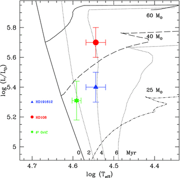
HR diagram with the position of HD 108 (red circle), HD 191612 (blue triangle) and θ1 Ori C (green asterisk) indicated. Evolutionary tracks include stellar rotation and are from Meynet & Maeder (2003). Isochrones are shown as dotted lines. Stellar parameters for HD 191612 and θ1 Ori C are from Walborn et al. (2003) and Simón-Díaz et al. (2006), respectively.
The comparison of the results of this study to those by Nazé et al. (2008) shows that the derived stellar parameters are in rather good agreement in spite of the difficulties encountered in the present analysis. Only the luminosity is marginally higher in this study [but the method we used for its determination is more accurate than in Nazé et al. (2008)]. This overall similarity demonstrates that the variability altering the shape of the optical lines is probably not due to changes in the star's stellar parameters. Instead, they might be related to the wind or immediate environment of the star.
4.2 Wind parameters
We relied on strong extreme ultraviolet and far-ultraviolet (FUV) lines to constrain the mass-loss rate ( ) and the terminal velocity (v∞). We avoided the use of wind-sensitive optical lines (Hα and He iiλ4686) since they show a high degree of short-term variability and can be contaminated by non-stellar emission.
We used only the FUSE LiF2A channel of the FUSE spectra in our analysis since wavelengths shorter than 1100 Å are heavily contaminated by the interstellar medium. Our best fit is shown in Fig. 4 (upper panel) and the corresponding parameters are listed in Table 3. The synthetic P v λλ1118, 1128 and Si iv λλ1122, 1128 lines are somewhat weaker and narrower than observed. By decreasing the mass-loss rate we tend to decrease this discrepancy, but a worse fit is achieved to the C iiiλ1176 and C ivλ1169 transitions.
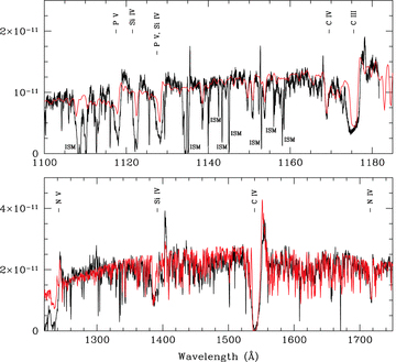
UV and far-UV observed spectra (black) and our final CMFGEN model (red). Top: FUSE LiF2A spectrum. Bottom: IUE spectrum. The region below 1200 Å common to the FUSE spectrum is very noisy and is not shown. The flux is in units of erg s−1 cm−2Å−1.
Unfortunately, no FUV spectra (1200–2000 Å) exist for the ‘low’ optical state. The only IUE observations cover the period 1978–1989 and are quite similar, showing no signs of significant variability. They presumably correspond to HD 108's ‘high’ optical state (the Balmer lines being in emission at least between 1987 and 1989; see Underhill 1994; Nazé et al. 2001). However, we found out that the set of parameters derived from the FUSE spectra leads to a good fit of the IUE data (see the lower panel of Fig. 4). We thus conclude that the global wind properties of HD 108 do not vary significantly between the low and high states. In particular, the mass-loss rate does not differ by more than a factor of 2 (corresponding to the uncertainty on our determination). We note that the wind parameters are also consistent with those derived by Nazé et al. (2008) who used the same IUE data but different optical spectra.
Given that the wind properties do not seem to depend on the star's state (high or low), we used N ivλ1718 to constrain the clumping factor (see a complete description in Bouret, Lanz & Hillier 2005). A small f value (0.01) corresponding to a large degree of wind inhomogeneities was necessary to correctly reproduce the blue wing extension.
4.3 Rotational velocity and macroturbulence
We used the Fourier transform method to constrain the projected rotational velocity (Gray 1992). To avoid any problem caused by wind and/or circumstellar emission, we selected photospheric lines showing the least degree of contamination. It turned out that no line showed a pure symmetric profile. Even for the best candidate features, the blue wing clearly showed a wider extension than the red wing, indicating some kind of contamination, most likely due to the wind. Consequently, we decided to work on an artificial, symmetric line profile created from the red wing of C ivλ5812, which we assume better reflects the true photospheric properties. We used the average of the 2009 July–August NARVAL spectra as input. No minimum was seen in the Fourier transform above the noise level, indicating that (1) the maximum v sin i compatible with our artificial profile is ∼50 km s−1 and (2) macroturbulence is an important broadening mechanism. Tests run on N ivλ4057 and O iiiλ5592 gave similar results. Note that the origin of macroturbulence in O stars is widely unknown, although Aerts et al. (2009) recently claimed that non-radial pulsations could be an important ingredient.
To further investigate the rotational velocity and to quantify the amount of macroturbulence, we used a synthetic line profile (taken from the TLUSTY OSTAR2002 grid of models). We artificially scaled it in order to match the equivalent width of the observed C ivλ5812 line. Since macroturbulence is the main broadening mechanism (see below) this is justified, the intrinsic profile being unimportant. We subsequently convolved this synthetic profile with (1) a rotational profile (characterized by v sin i) and (2) a pure Gaussian profile [characterized by its full width at half-maximum (FWHM) and the corresponding macroturbulence velocity vmac]. The latter mimics the effect of isotropic turbulence. Several (v sin i/FWHM) combinations were used and compared to the artificial profile described above. We found that rotational velocities larger than about 50 km s−1 are indeed excluded and that a macroturbulence larger than ∼30 km s−1 was necessary to reproduce the wings’ slope and extension. Different combinations of (v sin i/vmac) gave fits of similar quality. Fig. 5 shows three examples with v sin i= 0, 50 and 80 km s−1 and the corresponding vmac= 45, 38 and 0 km s−1. HD 108 is therefore very similar to HD191612 (Howarth et al. 2007) which also features macroturbulence-dominated line profiles.
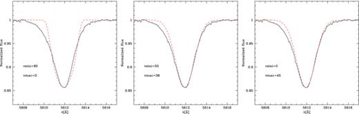
Comparison of the C ivλ5812 line with synthetic profiles with the following v sin i/vmac values (in km s−1): 80/0 (left), 50/38 (middle), 0/45 (right). The black solid line is the observed profile and the red dashed line the synthetic profile. While v sin i larger than 50 km s−1 is excluded, any value below this limit gives a satisfactory fit to the red wing provided a significant amount of macroturbulence is included.
5 DISCUSSION
The analogy between HD 108 and θ1 Ori C/HD 191612 suspected in Section 1 seems to be confirmed by this study. In particular, the similarity with HD 191612 is striking. Both stars show the same long-term spectroscopic variability, with He i and Balmer lines (other than Hα) changing from P Cygni to absorption-dominated profiles (see table 6 of Nazé et al. 2001). Howarth et al. (2007) reported a strong correlation between Hα emission and photometry, HD 191612 being brighter in the ‘high’ state. Barannikov (2007) provides evidence for the same behaviour of HD 108: photometry over the last 15 yr reveals a fading of HD 108 in parallel to a decrease of the emission component of He i and Balmer lines (see also Nazé et al., in preparation).
A notable difference is the variability time-scale. While a period of 538 d is identified for HD 191612, a value of several decades is preferred for HD 108. This rough estimate relies on two facts. First, the photometric survey of Barannikov (2007) discussed above points to a time-scale of at least 15 yr (and of at least 30 yr assuming roughly sinusoidal photometric variations). Secondly, a transition between absorption/P Cygni of several line profiles was observed at least twice during the last century, pointing to a periodicity of about 50–60 yr (see table 6 of Nazé et al. 2001). If, as suggested by Donati et al. (2006) for HD 191612, the variability time-scale corresponds to the rotation period, then HD 108 would be an extremely slow rotator with an equatorial velocity of ≲0.1 km s−1 (much lower than predicted by evolutionary models; see fig. 1 of Meynet & Maeder 2003). Our upper limit on the projected rotational velocity is fully consistent with this scenario. One might thus suspect that HD 108 experienced strong magnetic braking during its evolution.
Using the stellar and wind parameters derived in Section 4 and the minimum polar field discussed in Section 3, we obtain a confinement parameter  . Such a value implies that the wind of HD 108 is magnetically confined (ud-Doula & Owocki 2002). If the polar field is as large as that of HD 191612 (1.5 kG; see Section 3), this would imply η★∼ 800 and thus a strong wind confinement.
According to ud-Doula et al. (2009; see also discussion by Donati et al. 2006), the typical spin-down time-scale due to magnetic braking of a hot star with a strongly magnetically confined wind is  (k is a constant with a typical value of 0.1–0.3). For a kG polar field, this means τspin∼ 1–3 Myr. Given its Teff and luminosity, HD 108 is 3–5-Myr old (see Fig. 3). According to this simple estimate, the rotation rate of HD 108 could have been reduced by a factor of 3–200 just by magnetic braking (implying an initial rotational velocity from a few to 20 km s−1). However, tailored simulations relying on additional observations providing a better characterization of the field strength and geometry are obviously required to quantitatively tackle the question of magnetic braking (Maeder & Meynet 2005; ud-Doula et al. 2009).
The spectrum of HD 108 is varying on time-scales of a few decades. Our excellent time coverage in 2009 allows us to investigate the existence of faster variability. Fig. 6 shows a selection of He i, He ii and Balmer lines together with the corresponding temporal variance spectrum (TVS; see Fullerton, Gies & Bolton 1996) which quantifies the degree of variability. All He i and Balmer lines are variable on time-scales of days. He iiλ4686 also shows fluctuations. But the He ii λλ4200, 4542 lines (as well as C iv λλ5801–5812 and O iiiλ5592, not shown in Fig. 6) are stable over time. The He i and Balmer lines, as well as the wind line He iiλ4686, are formed over a large fraction of the atmosphere (i.e. photosphere + wind), especially if a disc/equatorial density enhancement exists. On the contrary, He ii λλ4200, 4542 are formed in the hottest part of the atmosphere, in or very close to the photosphere. The observed variability thus originates in the wind. Non-radial pulsations can thus be excluded since they would trigger variability in photospheric lines. A periodicity search performed on equivalent width measurements of several lines and using the Lomb–Scargle formalism did not reveal any pattern. We thus conclude that HD 108 presents day-to-day stochastic wind variability.
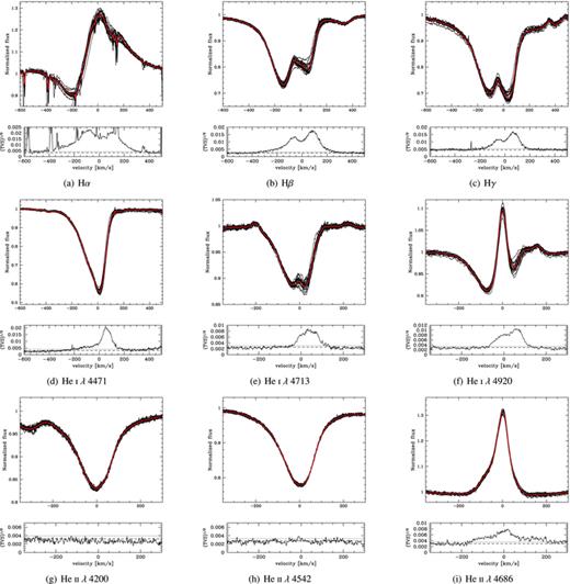
Line profile variability of Hα, Hβ, Hγ, He i λλ4471, 4713, 4920, He ii λλ4200, 4542, 4686 (panels a–i) between 2009 July 4 and October 9. The red bold line is the 2009 average spectrum, while the thin lines correspond to individual spectra. All spectra are shown in velocity space around the respective rest wavelength. The temporal variance spectrum (TVS; see Fullerton et al. 1996) is also given for each line (lower panels). The dot–dashed line shows the 1σ deviation of the continuum, while the dotted lines show the 99 per cent confidence limit. Variability is clearly detected in all Balmer and He i lines. On the contrary, the He ii lines are stable, with only a small variability in the wind line He iiλ4686.
In the standard magnetically confined wind scenario, and in the case of moderate to strong confinement, a disc is formed in the inner atmosphere (e.g. fig. 3 of ud-Doula & Owocki 2002). This disc is denser in its inner parts. ud-Doula & Owocki (2002) and ud-Doula, Townsend & Owocki (2006) have shown that in absence of sufficient centrifugal support, material accumulated in the disc and located below the corotation radius falls back on to the stellar surface (see fig. 4 of ud-Doula & Owocki 2002). This process is stochastic, and the disc is maintained dynamically by new material injected via the channelled wind. In most lines of Fig. 6, we see that variability is located preferentially on the red part of the profile. This can be interpreted as a direct evidence for the infall of ‘blobs’ of disc material. Indeed, density fluctuation along the line of sight will cause variation of the line strength, and the receding velocity will shift these variations towards longer wavelengths. We think that this variability in the red wings of most line profiles is an indication of material infall. Similar conclusions were reached by Wade et al. (2006) for θ1 Ori C. Hα seems to deviate from this scenario: its variability is located over the entire profile. Contrary to most lines of Fig. 6, Hα is formed further away from the photosphere and is usually more affected by the wind. It is known to be variable in a number of non-magnetic O stars, mainly due to the presence of inhomogeneities (‘wind clumping’) most likely due to hydrodynamical instabilities (e.g. Runacres & Owocki 2002). Markova et al. (2005) showed that such clumps could explain the Hα variability observed over the entire line profile of O supergiants. We thus suggest that in HD 108, Hα is formed in a zone where the putative disc of confined material is more tenuous than in the formation region of all other lines of Fig. 6. In that region, wind clumping affects the line profile in addition to material infall. This explains that variability is not confined to the red wing but is located over the entire profile. The large clumping factor derived in Section 4.2 (f= 0.01) is consistent with a very inhomogeneous wind. Obviously, more information on the field strength and geometry is needed to better constrain the wind confinement and to test our suggestion. In particular, better knowledge of the position of the Alfvén radius relative to the Hα formation region is important to test our hypothesis that Hα variability is at least partly caused by wind clumping.
It is also worth noting that the models of ud-Doula & Owocki (2002) and ud-Doula et al. (2006) consider only the case of magnetic axis aligned with the rotation axis. In our case, a tilt is likely present given the long-term line variability, so that the spin-down time-scale and centrifugal support cannot be strictly compared to the theoretical predictions.
We finally stress that in the case of magnetically confined winds, one might question the use of 1D atmosphere models to constrain the wind properties. However, it is unlikely that our mass-loss rate estimate is wrong by orders of magnitudes. Indeed, even if half of the material initially blown by radiative acceleration was to fall back on to the stellar surface, strong signatures of infall such as inverse P Cygni profiles or redshifted absorption should be seen. Since the only evidence for infall is the line variability of absorption lines, we think our estimate of the mass-loss rate is realistic.
6 SUMMARY AND CONCLUSIONS
We have presented spectropolarimetric observations of the Of?p star HD 108 conducted with the NARVAL and ESPaDOnS instruments (at TBL and CFHT, respectively). 110 circularly polarized spectral sequences have been collected between 2007 and 2009. We report the clear detection of a Stokes V Zeeman signature stable on time-scales of days to months, but likely slowly increasing in amplitude on time-scales of years. We speculate that this time-scale is the same as that on which the Hα emission is varying and is equal to the rotation period of the star. The corresponding longitudinal magnetic field is of the order of 100–150 G, implying that the polar strength of the putatively dipolar large-scale magnetic field of HD 108 is at least 0.5 kG and most likely of the order of 1–2 kG.
The stellar and wind parameters of HD 108 have been derived through atmosphere modelling with the code cmfgen. The effective temperature was poorly constrained due to the surprisingly strong He i λλ4471, 5876 lines. Values of Teff in the range of 33 000–37 000 K were conservatively derived from the analysis of the remaining He i and the He ii lines. A mass-loss rate of the order of 10−7 M⊙ yr−1 was derived. The wind is found to be strongly clumped (f= 0.01). It is also significantly confined (η★≥ 100, possibly up to 800) by the magnetic field. HD 108 shows long-term variability in most He i and Balmer lines, with profiles changing from pure absorption to P Cygni on a period of a few decades. We suggest that this periodicity corresponds to rotational modulation. The (magnetic) equatorial density enhancement implied by the wind confinement would then be seen edge-on at minimum line emission and pole-on at maximum emission. The time-scale for magnetic braking computed with the derived stellar, wind and magnetic properties is consistent with the star's age. A slow rotation is also consistent with the low v sin i we derive. HD 108 might thus be an even more extreme case of a slowly rotating magnetic O star than HD 191612.
Short-term line profile variability is also observed in He i and wind-sensitive lines. Photospheric He ii lines are very stable. Lines formed just above the photosphere show evidence for infall, while the variability of lines formed in the outer wind is more typical of normal hot stars’ outflows. We suggest that in the inner wind, we are witnessing the infall of material channelled by the field lines to the magnetic equator and subsequently pulled back to the stellar surface by gravity.
Most of the suggestions discussed in Section 5 and summarized above are still speculative. Future monitoring of HD 108 is obviously needed to confirm the expected correlation between the variation of the longitudinal magnetic field and the long-term spectroscopic variability. If the few decades’ spectroscopic and photometric modulation corresponds to the rotational period, a complete mapping of the magnetic topology is not possible until a few decades. However, crucial information regarding the field strength and geometry can be gathered in the next years since we have just passed the phase of minimum emission. The field is thus expected to strengthen, making detection easier. Further constraints on the field morphology will help to see (1) if the slow rotation of HD 108 is really due to magnetic braking and (2) if the short-term variability is caused by dynamical phenomena predicted by current simulations of magnetically channelled winds.
This effort is part of the Magnetism in Massive Stars (MiMeS) international research programme aimed at characterizing magnetic fields in upper main-sequence stars.
The reduced chi-squared estimator quantifies how significantly the observed Zeeman signature departs from a null profile (i.e. V= 0).
We thank John Hillier for making his code cmfgen available and for constant help with it. We also thank the generous time allocation from the TBL TAC and the MagIcS initiative under which MiMeS is carried out. We acknowledge the help of the TBL and CFHT staff for service and QSO observing, respectively. GAW acknowledges Discovery Grant support from the Natural Science and Engineering Research Council of Canada (NSERC). JCB and WLFM acknowledge financial support from the French National Research Agency (ANR) through programme number ANR-06-BLAN-0105.
REFERENCES
Author notes
Based on observations obtained at the Télescope Bernard Lyot (TBL) and at the Canada–France–Hawaii Telescope (CFHT). CFHT is operated by the National Research Council of Canada, the Institut National des Sciences de l'Univers of the Centre National de la Recherche Scientifique of France (INSU/CNRS), and the University of Hawaii, while TBL is operated by CNRS/INSU.
