Resolved images of self-gravitating circumstellar discs with ALMA Free

Abstract

1 INTRODUCTION

Circumstellar discs play an important role in the formation and evolution of both stars and planets, and as such have been the object of much study and observation in recent years. Millimetre wavelength surveys of star-forming regions in Taurus (Beckwith et al. 1990; Kitamura et al. 2002; Andrews & Williams 2005), Orion (Eisner et al. 2008) and ρ Ophiuchus (Andre & Montmerle 1994; Andrews & Williams 2007a) have provided extensive evidence of circumstellar discs, while optical images have been provided by the Hubble Space Telescope (HST) of HH 30 (Burrows et al. 1996) and the Fomalhaut system (Kalas et al. 2008). However, relatively few systems have been imaged with great enough resolution to determine the disc structure on scales of less than a few tens of au.

This may be about to change, however, with the Atacama Large Millimetre/sub-millimetre Array (ALMA) due to come on line in the near future. With a minimum beam diameter of ∼5 mas at 900 GHz, ALMA should ideally provide resolution down to ≈2 au for discs observed in Orion, with sub-au resolution for systems in Taurus-Auriga. It will therefore allow observations of disc substructure in unprecedented detail. The discovery of structures within discs could have important implications for our understanding of the evolution of both the discs themselves (Rice & Armitage 2009) and the protostars they orbit.

Gaseous circumstellar discs are expected to be turbulent (Ebert 1994; Gammie 1996), with the internal stresses that this turbulence induces being the principal driver of angular momentum transport and thus accretion. This turbulence will lead to substructure being present at all scales within the disc, with those on smaller scales (due to the magnetorotational instability) remaining undetectable, while the larger scale structure induced by the gravitational instability should be resolvable with ALMA.

It is expected that protostellar discs about Class 0/Class I objects will go through a self-gravitating phase (Bertin & Lodato 2001; Vorobyov & Basu 2005; Hartmann 2009) as the infall rate from the gaseous envelope is much greater than the accretion rate on to the protostar (Vorobyov & Basu 2006). In this phase large-amplitude spiral structures will form, driving accretion on to the protostar (Lin & Pringle 1987; Laughlin & Bodenheimer 1994; Armitage, Livio & Pringle 2001; Lodato & Rice 2004, 2005) and potentially leading to the formation of companion objects. These companions may vary in size from stellar mass (Bonnell 1994; Bonnell & Bate 1994; Whitworth et al. 1995) to brown dwarf or planetary mass (Rice, Lodato & Armitage 2005; Stamatellos, Hubber & Whitworth 2007; Clarke 2009; Cossins, Lodato & Clarke 2010). It is possible that protoplanetary discs around Classic T Tauri (Class II) stars may also exhibit spiral patterns due to the presence of gravitational instabilities (Bertin & Lodato 2001; Boley et al. 2006; Vorobyov & Basu 2008; Cossins et al. 2010), and indeed there are already possible detections of spiral structures in the discs of GSS 39 in Ophiuchus (Andrews et al. 2009) and in IRAS 16293−2422B (Rodríguez et al. 2005).

At radii greater than ∼50 au, planet formation through direct fragmentation of these spiral overdensities into bound objects is possible (Boss 1997, 1998; Clarke 2009; Rafikov 2009; Cossins et al. 2010). While Wolf & D'Angelo (2005) have indicated that the forming giant (proto-) planets themselves may be detectable using ALMA, the observability of the large-scale spiral structure itself within protostellar and protoplanetary discs, though implied (Testi & Leurini 2008), has remained undemonstrated. (Note however that Krumholz, Klein & McKee (2007) have discussed the ALMA observability in molecular lines of very large-scale spirals (∼10³/au), expected to characterise discs around massive stars.) In this paper, we therefore present a simple self-gravitating disc simulation, and from it we derive mock observations of disc systems at the resolutions and sensitivities that should be possible with ALMA. Hence in Section 2 we detail the simulation, and in Section 3 we discuss how the mock observations are generated from it, taking into account telescope effects and sensitivities. In Section 4 we present the observations for various system and telescope parameters, and finally in Section 5 we discuss the significance of our results.

2 NUMERICAL SIMULATION OF STRUCTURE FORMATION

Gravitational instabilities in discs have been extensively studied numerically using both grid-based Eulerian codes (Gammie 2001; Pickett et al. 2003; Boley et al. 2006; Kratter et al. 2010) and Lagrangian particle-based methods (Rice et al. 2003; Lodato & Rice 2004, 2005; Nayakshin, Cuadra & Springel 2007; Alexander, Armitage & Cuadra 2008; Cossins, Lodato & Clarke 2009; Forgan & Rice 2009), and the reader is referred to these for further details of the dynamics of gravitationally unstable discs. The simulation we use to generate the mock observations was performed in the manner detailed in Cossins et al. (2009) using a 3D smoothed particle hydrodynamics (sph) code, a Lagrangian hydrodynamics code capable of modelling self-gravity (see e.g. Benz 1990; Monaghan 1992, 2005; Price & Monaghan 2007). Our system consists of a single point mass orbited by 500 000 sph gas particles, with the central object free to move under the gravitational influence of the disc. All particles evolve according to individual time-steps governed by the Courant condition, a force condition (Monaghan 1992) and an integrator limit (Bate, Bonnell & Price 1995).

We allow the discs to cool towards gravitational instability by implementing a simple cooling law of the form

1

where u_i and t_cool,i are the specific internal energy and cooling time associated with the i th particle. We then determine the cooling time t_cool through the simple prescription that

2

where Ω is the angular frequency and β is a fixed parameter throughout each simulation. Although this is clearly an ad hoc cooling function, it can be used as a simple parametrization in order to conduct controlled numerical experiments. In Cossins et al. (2009) we found that for a given disc mass, the spiral structures formed through the gravitational instability (as characterized by the radial and azimuthal wavenumbers of the excited modes) are independent of the cooling, but that the strength of the modes (characterized by the relative rms amplitude of the surface density perturbations 〈δΣ/Σ〉) varies such that

3

Therefore, notwithstanding the simplicity of our cooling prescription, we may reasonably assume that the spiral structures formed in physical systems with characteristic masses corresponding to those in our simulation will have qualitatively similar structure formation, with the uncertainty lying primarily in the amplitudes of the density perturbations.

Furthermore, in Cossins et al. (2010) we characterize the behaviour of Ωt_cool with radius and show that for accretion rates of ∼10⁻⁷ M_☉ yr⁻¹ (typical for Classic T Tauri objects) at radii of 20–50 au the value of Ωt_cool is ∼10¹–10², decreasing with increasing radius. Hence, although the cooling formalism given in equation (2) is very simple, it produces spiral structure in the correct modes and at approximately the correct amplitudes for the outer radii of discs, as long as we choose β in the range of ≳10. It is therefore useful as a means of generating test cases to investigate whether such structures would actually be observable, particularly in the outer parts of discs.

2.1 Simulation details

The simulation used to generate the mock observations described here consists of a 0.2-M_☉ disc about a 1.0-M_☉ mass star, extending out to ∼25 au. Although this is a relatively high mass ratio, it is within observed bounds (Andrews & Williams 2005, 2007a) and is plausible for the early (Class I) stages of intermediate-mass protostellar evolution, when the disc is expected to be self-gravitating (Bertin & Lodato 2001; Vorobyov & Basu 2005; Hartmann 2009).

Our initial conditions consist of a disc of gas particles on circular orbits, distributed with a surface density profile Σ∼R^−γ with γ= 1.5, as for the minimum mass solar nebula (MMSN; Weidenschilling 1977). Note that observational constraints for γ range from 0.4 ≲γ≲ 1.0 for protoplanetary discs in Ophiuchus (Andrews et al. 2009) to 0.1 ≲γ≲ 1.7 in Taurus (Andrews & Williams 2007b), so this value is within observed limits.

The disc is initially in approximate vertical hydrostatic equilibrium with a Gaussian distribution of particles where the scaleheight H=c_s/Ω and c_s is the sound speed. The azimuthal velocities take into account both a pressure correction (Lodato 2007) and the enclosed disc mass, and any variation from dynamical equilibrium is washed out on the dynamical time-scale. The initial temperature profile is such that c²_s∼R^−1/2, with the minimum value of the Toomre parameter Q_min= 2 occurring at the outer edge of the disc. In this manner, the disc is initially gravitationally stable throughout its radial range.

Note that the sph code and the initial conditions used are exactly the same as were used in Lodato & Rice (2004, 2005) and Cossins et al. (2009, 2010), excepting the fact that here we have used a mass ratio of 0.2, and the reader is directed to these for further details. Finally, in terms of cooling, we set β= 7 and use the cooling formalism described in equation (1). This is approximately in the expected range and is low enough to avoid spurious numerical heating effects due to artificial viscosity (Lodato & Rice 2004).

2.2 Disc evolution

Although the thermal profile of the disc initially ensures that it is gravitationally stable at all radii, it is however not in thermal equilibrium. As the simulation evolves, the disc therefore cools towards gravitational instability, which is initiated when Q≈ 1, after ∼1000 yr. The disc then settles into a marginally stable, quasi-steady dynamic thermal equilibrium state, characterized by the presence of spiral density waves that propagate across the face of the disc and which provide heat (through shocks) to balance the imposed cooling. These spiral waves are clearly seen in the surface density, as shown in Fig. 1. The simulation was run for ∼10 000 yr (equivalent to ∼10 cooling times at the disc outer edge), suggesting that during the self-gravitating period of protostellar evolution (expected to last a few ×10⁵ yr during and immediately after the infall phase) circumstellar discs should indeed be able to reach this quasi-steady state. Since the surface density varies on the longer viscous time-scale, the original Σ∼R^−3/2 profile remains largely unchanged throughout the simulation.

Figure 1

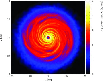
Simulated surface density perturbations in a 0.2-M_☉ disc about a 1.0-M_☉ protostar. The gravitationally induced spiral waves that impart heat to the disc are clearly visible.

Open in new tabDownload slide

Once the disc reaches the self-regulated dynamic thermal equilibrium state, the disc temperature falls to ∼20–40 K, with the minimum at the disc outer edge, as shown in Fig. 2. Between roughly 10 and 25 au the temperature falls off as R⁻¹, in reasonable agreement with observations (Andrews & Williams 2007b). Note that the slight temperature rise outside of R≈ 25 au is due to very low density, higher temperature gas external to the main bulk of the disc.

Figure 2

Azimuthally averaged temperature profile of the disc once it has settled into the dynamic thermal equilibrium state. The dashed line shows an R⁻¹ profile.

Open in new tabDownload slide

3 GENERATION OF MOCK OBSERVATIONS

Having run the hydrodynamic simulations, it is then necessary to use the disc parameters to create flux maps of the objects as they may appear using ALMA. Throughout the following, we assume that the disc is face-on to the observer.

In order to calculate the emission, we use the individual particle densities ρ_i generated from the sph simulations and calculate the particles' absorption coefficients α_ν,i at frequency ν using

4

where κ_ν is the opacity of the disc at frequency ν.

For a face-on disc, the optical depth τ_ν at frequency ν is defined in the following manner:

5

and hence for a disc of SPH particles, we may evaluate the vertical optical depth at any point on the disc face by approximating this integral as a sum over all the relevant interacting particles. We therefore use the following approximation for the optical depth of the disc as seen by a distant observer:

6

where w_i is a weighting function related to the particle's mass, density and the sph smoothing kernel (see Price 2007) and where i denotes all particles along a given line of sight through the disc.

We assume that radiation from the disc is in thermal equilibrium with itself and thus that the disc emits as a blackbody, with the source function S_ν at frequency ν given by the Planck function:

7

where h is Planck's constant, c is the speed of light in vacuo, k is Boltzmann's constant and T is the temperature of the emitter. For simplicity, we assume that our discs are vertically isothermal with temperature T (which we obtain via a vertical average from the simulations), meaning that at each point in the disc the source function is constant with height, and is given by B_ν(T). Modelling the disc in this manner, as a geometrically thin structure with no vertical temperature gradient, is obviously a very crude approximation. Nevertheless, since we are only interested in predicting the emission in the (sub-) mm range, this approximation is justified as the bulk of the emission will indeed come from the relatively isothermal layer located about the disc mid-plane.

For such a constant source function, the specific intensity (or surface brightness) I_ν at frequency ν and optical depth τ_ν is given by

8

Note that this formulation for the surface brightness is often used in reverse to infer disc properties from the (sub-) mm surface brightness (e.g. Beckwith et al. 1990; Andrews et al. 2009). Furthermore, it is also clear that once the disc becomes optically thick its emission is determined solely by its temperature, whereas in optically thin regions the emission is exponentially dependent on τ_ν. Optically thick structures forming in optically thin parts of the disc are therefore likely to show greater variation in intensity (and thus be more readily observable) than structure in purely optically thick regions.

3.1 Dust opacities

A critical parameter in the above calculation is the opacity of the disc κ_ν. At temperatures below ≈160 K the Rosseland mean opacity becomes dominated by ices (Bell & Lin 1994; Cossins et al. 2010), but the specific value of the opacity at a given frequency κ_ν is determined by the grain size distribution (Miyake & Nakagawa 1993).

To determine the value of κ_ν, we use the power-law model of Beckwith et al. (1990), such that

9

where ν₁₂= 10¹² Hz and κ₁₂ is the value of the opacity at this fiducial frequency. The normalization constant κ₁₂ is relatively poorly constrained, with values ranging from 0.1 (Beckwith et al. 1990) to ∼0.016 cm² g⁻¹ (Kramer et al. 1998; Rafikov 2009). For protoplanetary and protostellar discs, the power-law index β can be determined from the disc spectral energy distribution in the mm/sub-mm range and is found to be in the region 0.3 ≲β≲ 1.5 (Kitamura et al. 2002; Testi et al. 2003; Ricci et al. 2009). Note that this range is below that expected for the interstellar medium β≈ 1.7–2 (Finkbeiner, Davis & Schlegel 1999; Chakrabarti & McKee 2008; Hartmann 2009), which is attributed to grain processing within the disc.

For our models we use a fiducial dust opacity κ₁₂= 0.025 cm² g⁻¹, and in accordance with Rafikov (2009) we assume throughout that β= 1.0, such that

10

3.2 The ALMA simulator

To produce realistic simulated ALMA observations of the models, we have used the ALMA simulator simdata in Common Astronomy Software Applications (CASA).1 The version of the simulator we used (2.4) allows us to use the latest version of the planned ALMA antenna configurations, the expected receiver noise based on technical specifications and the contribution due to the atmosphere, itself based on input values for the atmospheric temperature T_atm and the optical depth at the frequency of the simulations. In all the simulations presented here we assume T_atm= 265 K, and the optical depth is computed using the ATM atmosphere models of Pardo, Cernicharo & Serabyn (2002). We use typical Chajnantor conditions and an amount of precipitable water vapour (pwv) as expected for dynamical scheduling of the observations. In Table 1, we therefore show the water content and opacity of the atmosphere, the expected theoretical noise and the angular and linear resolutions of the simulations for discs at 50 and 140 pc for each frequency.

Note that we have also run simulations for the lowest (45 GHz) and highest (870 GHz) planned ALMA bands – contrary to the intermediate frequencies, these frequency bands will not be available when ALMA first comes online. High-frequency receivers are planned to be introduced during the early years of ALMA science operations, while the low-frequency band is under discussion for the ALMA development programme.

The array configuration used varied for each frequency, as we aimed to use the configuration that offered the best compromise between surface brightness sensitivity and angular resolution. Note that at low frequencies, the angular resolution is limited by the largest available array configuration. In all cases, we performed aperture synthesis simulations with a transit duration of 2 h.

4 RESULTS

Using the disc simulation shown in Fig. 1, we investigated the emission at the various frequencies shown in Table 1. Based on the requirement that the optical depth should vary between optically thick in the spiral arms and optically thin in the interarm regions (to maximize the contrast in emission across these regions), we have principally considered the results at 345 GHz. Furthermore, at this frequency we expect the resolution to be roughly 1 au at both TW Hydrae (TW Hya) and Taurus-Auriga distances, while the telescope sensitivity should not be a limiting factor. To illustrate the effects of varying the frequency, the optical depth at 45, 345 and 870 GHz is shown in Fig. 3 for comparison. Also clear from this figure is the expected increase in optical depth with frequency due to increasing opacity.

Figure 3

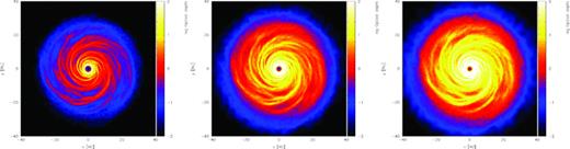
Comparison of the (logarithmic) optical depth across the disc face at frequencies of 45 GHz (left), 345 GHz (centre) and 870 GHz (right). The greatest contrast between optically thick and optically thin regions across the arm/interarm regions in the bulk of the disc is to be seen in the 345-GHz case.

Open in new tabDownload slide

4.1 Simulated ALMA images

Having generated the specific intensity map by the method described in Section 3, we have used them to simulate ALMA observations as described in Section 3.2. In Figs 4 and 5, we therefore show the results of our simulations for discs at a distance of 50 pc (TW Hya) and 140 pc (Chamaeleon, Ophiuchus, Taurus-Auriga). Note that our simulations only include the effects of thermal noise from receivers and the atmosphere but do not take into account calibration uncertainties and residual phase noise after calibration. These effects are likely to be most important at high frequencies and long baselines, so the simulated maps at 680 and 870 GHz, especially for the 140-pc case, represent observations carried out in ideal conditions and with excellent calibrations.

Figure 4

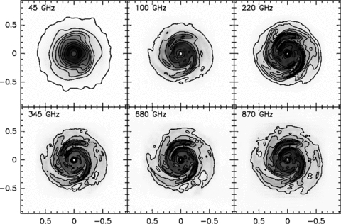
Simulated aperture synthesis ALMA images for a disc at 50 pc, with a transit duration of 2 h. From left to right and top to bottom, we show simulations computed for an observing frequency of 45, 100, 220 (top) and 345, 670 and 870 (bottom) GHz. Axis scales are in arcseconds. Contours start at 0.01 and are spaced by 0.08 mJy beam⁻¹ at 45 GHz, start at 0.08 and are spaced by 0.2 mJy beam⁻¹ at 100 GHz, start at 0.5 and are spaced by 0.5 mJy beam⁻¹ at 220 GHz, start at 0.8 and are spaced by 0.8 mJy beam⁻¹ at 345 GHz, start at 2 and are spaced by 2 mJy beam⁻¹ at 680 GHz, start at 4 and are spaced by 4 mJy beam⁻¹ at 870 GHz.

Open in new tabDownload slide

Figure 5

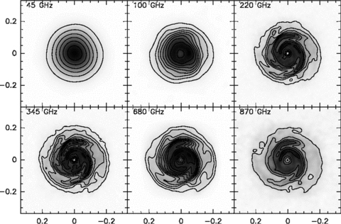
As for Fig. 4, but for a disc at 140 pc. Contours start at 0.08 and are spaced by 0.08 mJy beam⁻¹ at 45 GHz, start at 0.08 and are spaced by 0.08 mJy beam⁻¹ at 100 GHz, start at 0.1 and are spaced by 0.1 mJy beam⁻¹ at 220 GHz, start at 0.2 and are spaced by 0.2 mJy beam⁻¹ at 345 GHz, start at 2 and are spaced by 1 mJy beam⁻¹ at 680 GHz, start at 1 and are spaced by 1 mJy beam⁻¹ at 870 GHz.

Open in new tabDownload slide

The simulations show that the predicted spiral structure is readily detectable at all simulated frequencies at the 50-pc distance of the TW Hya association. In the case of star-forming regions at 140 pc, the situation is less clear-cut. At low frequencies (≲100 GHz), even ALMA will probably not provide the angular resolution required to image the spiral structure clearly, whereas at the highest frequencies, as noted above, the simulations are probably over-optimistic. Nevertheless, our simulations show that at 220 and 345 GHz (ALMA Bands 6 and 7), the predicted structures should be clearly detectable.

Finally, in Fig. 6 we show the predicted observability of a disc at 410 pc (equivalent to the Orion Nebula Cluster distance) imaged at 345 GHz. While the non-axisymmetric nature of the disc is clear, the spiral structure per se is not well resolved, and thus we infer that even with ALMA such structures will not be conclusively detectable.

Figure 6

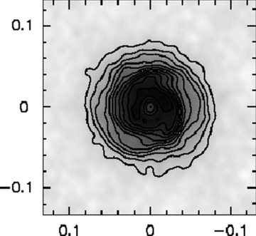
Simulated 345-GHz aperture synthesis image of a disc at 410 pc, with a transit duration of 2 h. Contours start at and are spaced by 60 mJy beam⁻¹. Clear asymmetries are present, but the underlying spiral structure is not well resolved.

Open in new tabDownload slide

5 DISCUSSION

In this paper, we have used a 3D, global SPH simulation of a massive (0.2-M_☉) compact (R_out= 25 au) self-gravitating disc about a young star (1.0 M_☉) to demonstrate that the spiral modes excited by the gravitational instability should be detectable in face-on circumstellar discs using ALMA. At distances comparable to the TW Hydrae association (∼50 pc), such spiral density waves are readily apparent with observation times of 2 h, whereas at Taurus distances of ∼140 pc, a careful choice of the observing frequency and excellent observing conditions may be required for significant detections. Our results suggest that structure in such discs in Orion (∼400 pc) will most likely not be resolvable.

In order to generate these predicted observations, we have used temperature and density maps provided by numerical simulations, together with an empirical relationship for the dust opacity of circumstellar material to obtain the optical depth at each part of the disc face. In a precisely similar manner to that used to obtain disc properties from sub-mm observations (Beckwith et al. 1990), we have then been able to determine the specific intensity of the disc emission across the disc face, which has then been used as input for the ALMA simulator in CASA to produce simulated observations. We find that observation frequencies of around 345 GHz (870 μm) are ideal for this kind of observation, as we find the spiral arms to be optically thick, whereas the interarm regions are optically thin, maximizing the contrast in emission between the regions. It should be noted however that this ‘ideal’ frequency range is dependent on our assumptions concerning the dust opacity, in which there is considerable scatter.

There are certain limitations to our model which should be noted, however. Our stellar and disc masses are both at the upper end of the expected distributions (Beckwith et al. 1990; Andrews & Williams 2005, 2007a), although in the early stages of star formation (Class I objects) such high disc masses are not unreasonable due to the infalling envelope. Of necessity, in order to be self-gravitating our discs are cold (20–40 K), which implies both a relatively low ambient temperature (not unreasonable, since giant molecular clouds tend to have temperatures of ∼10 K; Myers & Benson 1983; Myers, Linke & Benson 1983) and for heating from the protostar to be negligible. While this latter assumption is clearly unlikely to be valid for the surface layers of the disc that are irradiated directly by the star, the disc mid-plane (which dominates the emission) is likely to be cold enough to justify this assumption (D'Alessio et al. 1998; Andrews & Williams 2005; Dullemond et al. 2007). In a similar manner, this assumption of a colder inner layer allows us to ignore the effects of the magnetorotational instability (Gammie 1996).

Given that our disc is quite compact, and many discs are observed to extend out to much larger radii (∼10²–10³ au; Kitamura et al. 2002; Andrews & Williams 2007a; Eisner et al. 2008; Andrews et al. 2009), the colder regions outside of ∼50 au are if anything more likely to show evidence of gravitational instability than at the radii we simulate, and indeed any spiral structures forming at large radii will be more easily resolvable. In this sense therefore our predictions may even be conservative in terms of the maximum distance at which spiral structures may be detectable.

Likewise our cooling prescription, although simplistic, is valid for regions at large radii where the temperature is below the ice sublimation temperature and is therefore not an unreasonable simplification. It should be noted that the ratio of the cooling time to the dynamical time β=t_coolΩ determines the amplitude of the spiral perturbation and hence the contrast in the simulated images. The value β= 7 adopted in this paper is in the right range for discs at a few tens of au. However, a larger value of β (i.e. a less efficient cooling) would provide a relatively smaller contrast in the ALMA images.

Finally, note that in this paper we have considered the contribution to the sub-mm emission due solely by the disc. In the earliest phases of star formation, the system might show a substantial emission on larger scales, produced by the infalling envelope feeding the disc. This larger scale contribution has been neglected in this paper.

As noted in Section 1, there are already possible detections of spiral structures in the discs of GSS 39 in Ophiuchus (Andrews et al. 2009) and in IRAS 6293−2422B (Rodríguez et al. 2005). However, the structures in GSS 39 are not robust at the 3σ level (Andrews et al. 2009), and those in IRAS 16293−2422B, whilst appearing to be genuine, may plausibly be due to interactions with a companion. Furthermore, the presence of planetary mass objects within the disc may also lead to the excitation of spiral density waves (see for instance Goldreich & Tremaine 1980; Ogilvie & Lubow 2002; Armitage & Rice 2005). However in this latter case, the one-armed spiral waves are in general tightly wound (dependent on the disc thickness; Ogilvie & Lubow 2002) and would therefore be difficult to detect directly. Furthermore, analysis by Wolf & D'Angelo (2005) on the observability of embedded gas giant planets using ALMA suggests that the spirals would only be visible very close to the planet itself. Any detections of large-scale spirals in isolated protostellar discs are therefore likely to be due principally to the action of the gravitational instability.

Confirmed, unambiguous observations of gravitationally induced spiral structures within protostellar discs would be valuable for a number of reasons. As the gravitational instability is expected to operate during the early phases of star formation, processing the infalling envelope and allowing rapid accretion on to the protostar, such detections would validate this mechanism for growing the masses of protostars. More controversially, it may enable models of brown dwarf/low-mass stellar companion formation through disc fragmentation (Bate, Bonnell & Bromm 2002; Stamatellos et al. 2007; Clarke 2009; Stamatellos & Whitworth 2009) to be validated, as the presence (or otherwise) and amplitudes of spiral arms would allow constraints to be placed on the numbers of such companions that may be expected.

In a similar vein, detections of spiral features may enable us to determine the dominant mode of planet formation at various radii, about which there is some debate. While the standard core-accretion model is favoured at low radii (Lissauer 1993; Bodenheimer, Hubickyj & Lissauer 2000; Klahr 2008; Boley 2009), direct fragmentation of gravitationally induced spirals remains a candidate mechanism at radii above ∼50 au (Boss 1997; Boley et al. 2006; Rafikov 2009; Cossins et al. 2010). As the presence of a peak in the 1.3-cm emission around HL Tau has been put forwards as a promising candidate for a planetary mass companion formed through gravitational instability, detections of the spiral wave progenitors of such companions would provide significant backing for this mechanism. Moreover, the presence of large-amplitude spiral density perturbations may be important for the formation and growth of planetesimals, both due to the concentration of the dust fraction within the arms (Rice et al. 2004, 2006; Clarke & Lodato 2009) and due to the possible scattering of planetesimals by the spiral potential (Britsch, Clarke & Lodato 2008). In either case, observations of the spiral arms themselves would place constraints on, and therefore allow us to discriminate between, the two planet formation modes at large radii.

We acknowledge the use of splash (Price 2007) for the rendering of all surface density and optical depth plots. PC would further like to thank Mark Wilkinson for helpful discussions concerning observational techniques. LT would like to thank R. Indebetouw at NROA for developing, updating and maintaining the ALMA simulator in CASA.

REFERENCES