Tight constraints on the existence of additional planets around HD 189733* Free

Abstract

1 INTRODUCTION

Ground-based radial velocity and photometric transit surveys have proved to be the most successful methods for discovering exoplanets over the past decade, yielding more than 400 extrasolar planets discovered to date.1 Most of the exoplanets detected are of Jupiter mass, but Earth-mass planets remain to be found. An additional planet in a transiting system will perturb the motion of the transiting planet, and the interval between the mid-eclipses will not be constant. Deviations from the predicted mid-transit times can therefore reveal the presence of other bodies in the system, or place limits on their existence. Short-term variations can uncover the existence of other planets (Agol et al. 2005; Holman & Murray 2005), moons (Sartoretti & Schneider 1999; Kipping 2009) and also Trojans (Ford & Holman 2007), whereas long-term variations result from orbital decay (Rasio et al. 1996) and from orbital precession induced by another planet, stellar oblateness and general relativistic effects (Miralda-Escudé 2002; Heyl & Gladman 2007). Discovery of additional bodies can constrain theories of planetary system formation and evolution. In this paper, we describe a transit timing study of the transiting exoplanet system HD 189733.

The HD 189733 transiting system is one of the best-studied systems from the ground. HD 189733 is a bright star with magnitude V= 7.67 which is orbited by a transiting Jupiter-mass planet in a period of ∼2.22 days (Bouchy et al. 2005), and which also has a distant mid-M dwarf binary companion (Bakos et al. 2006a). In 2006, HD 189733 was observed with the Microvariability and Oscillations of Stars (MOST) satellite and these data were used to search for the existence of other bodies in the system. First, Croll et al. (2007) searched for transits from exoplanets other than the known hot Jupiter, with the result that any additional close-in exoplanets on orbital planes near that of HD 189733b with sizes ranging from about 1.7 to 3.5 R_⊕, where R_⊕ is the Earth radius, are ruled out. Secondly, an analysis of transit timing variations (TTVs) in these data has been carried out by Miller-Ricci et al. (2008) who found that there are no TTVs greater than ±45 s, which rules out planets of masses larger than 1 and 4 M_⊕, where M_⊕ is the Earth mass, in the 2:3 and 1:2 inner resonances, respectively, and planets greater than 20 M_⊕ in the outer 2:1 resonance of the known planet and greater than 8 M_⊕ in the 3:2 resonance.

Analyses of transit times similar to Miller-Ricci et al. (2008) have been carried out for other transiting planetary systems. Steffen & Agol (2005) found no evidence for a second planet in the TrES-1 system, excluding planets down to Earth mass near the low-order, mean-motion resonances of the transiting planet. Similarly, Gibson et al. (2009, 2010) found no evidence for additional planets down to sub-Earth masses in the interior and exterior 2:1 resonances of the TrES-3 and HAT-P-3 systems.

To measure times of mid-transits with sufficient accuracy to detect terrestrial mass planets requires high-quality photometry, free of systematic effects. HD 189733 is known to have surface spots; Pont et al. (2007) observed two spot events in Hubble Space Telescope (HST) data when the flux during the transit changed by 1 and 0.4 mmag. The presence of surface spots on HD 189733 complicates any transit timing analysis (Miller-Ricci et al. 2008). The light curve can be distorted if the planet transits in front of a spot or due to intrinsic variability of the star. The system parameters and the mid-eclipse times derived can then be affected by an inappropriate fitting model.

Instrumental effects during transit ingress or egress can also influence the accuracy and determination of transit times. For example, if the transit light curve is not properly normalized so that all data points in egress have a flux level that is slightly too high, the transit time will be determined too early. Correct normalization is especially problematic for partial transit light curves. Both instrumental effects and stellar variability can cause that a light curve is improperly normalized.

It is also important to have a light curve that is well sampled during both ingress and egress, because the transit timing information is contained in these parts. When using large telescopes for such a bright star, only short exposure times are needed to get sufficient signal-to-noise ratio and to avoid saturation, and so the cadence of observation is higher. For a given data accuracy, higher cadence leads to more accurately determined transit times.

In Section 2, we describe our observations, and in Section 3 we present our data reduction. In Section 4, we explain the techniques used to estimate uncertainties in our data and to measure the system parameters. Finally, in Section 5 we describe the three-body simulations used to place limits on the existence of other bodies in the system, and we conclude and discuss our results in Section 6.

2 OBSERVATIONS

We observed eight full and two partial transits of HD 189733 with the 2.6-m Nordic Optical Telescope (NOT), La Palma, Spain, using the Andalucia Faint Object Spectrograph and Camera (ALFOSC), and two full transits using the AG2 camera on the 4.2-m William Herschel Telescope (WHT) of the Isaac Newton Group (ING), La Palma, Spain (Table 1).

The ALFOSC has a 2048 × 2048 back-illuminated CCD with scale 0.19 arcsec pixel⁻¹ and field of view (FOV) 6.5 × 6.5 arcmin². To reduce the readout time of each exposure and the duty cycle of observation, we windowed the CCD with the window sizes summarized in Table 1. We used a Strömgren y filter to minimize effects of colour-dependent atmospheric extinction on the differential photometry and the effect of limb darkening on the transit light curves. We defocused the telescope typically to 3.4 arcsec, spreading the light inside full width at half-maximum (FWHM) of the point spread function (PSF) over ∼250 pixels, in order to minimize the impact of pixel-to-pixel sensitivity variations and to prevent saturation. Exposure times were chosen to keep counts below 50 000 per pixel to avoid saturation of features such as hotspots and speckles in the defocused stellar images, and to ensure data linearity. The typical exposure time for the NOT data was 3 s (Table 1).

AG2 is a frame-transfer CCD mounted at the WHT's folded Cassegrain focus, based on an ING-designed autoguider head. The FOV is 3.3 × 3.3 arcmin² and the scale is 0.4 arcsec pixel⁻¹. We used a Kitt Peak R filter and defocused the telescope to 10 and 12 arcsec for the two nights, spreading the FWHM light over ∼490 and 700 pixels, respectively. The corresponding exposure times were 10 and 3 s.

The mid-time of each exposure was converted to the Barycentric Julian Date (BJD) using the program barcor.2 We use BJD throughout this paper, because for this system the Heliocentric Julian Date would accumulate an error of up to 4 s.

3 DATA REDUCTION

Bias subtraction, flat-field correction and aperture photometry were performed using the Image Reduction and Analysis Facility (iraf)3 procedures.

To ensure a signal-to-noise ratio in excess of 1000 in our Strömgren y-filter flat fields for the NOT data, we generated a master flat field for each night using individually weighted normalized flat fields from the entire observing season combined with weights W= 1 −D/S, where D is the time interval between each night and date of observation and S is the season length. Applying flat-field corrections has only a minor effect on the resulting NOT photometry, because of the heavily defocused PSF.

For the WHT data, we determined master flat fields with a signal-to-noise ratio greater than 1 000 for both nights. However, we identified a position-angle-dependent scattered light component in the flat fields, which introduced systematic noise in our WHT photometry. Therefore, we did not apply flat-field corrections.

We used the star 2MASS 20003818+2242065 as our comparison star for the WHT data. In our NOT data, there are two available comparison stars, 2MASS 20003818+2242065 and 2MASS 20003286+2241118. We found the ratio of their measured intensities varies by a few mmag with time, as the telescope tracks across the meridian. This variation correlates with small drifts in the positions of the stars on the CCD, suggesting that some light is being lost from the aperture around one of the stars due to the wings of the PSF drifting out of that aperture. A similar variation is seen for the ratio of the intensities of 2MASS 20003286+2241118 and out-of-transit HD 189733, but not for 2MASS 20003818+2242065 and HD 189733, suggesting that it is light from 2MASS 20003286+2241118 which is being lost. This star is the farther of the two from HD 189733, and we conclude that the variation in measured intensity is due to a combination of the small drifts in stellar position on the CCD, and the variation of the defocused PSF across the FOV. We therefore used only the comparison star which is closer to HD 189733.

We used circular, equal diameter, photometric apertures for both HD 189733 and the comparison star. A range of aperture sizes was tried and that producing the minimum noise in the out-of-transit data was adopted and fixed during each night. The aperture radius for all stars ranged from 18–29 pixels for different NOT nights and the typical FWHM was around 18 pixels (3.4 arcsec). For the two WHT nights, the aperture radius was 28 and 30 pixels, respectively, and the corresponding FWHM was 25 and 30 pixels (10 and 12 arcsec).

We ensured the apertures tracked small drifts in the stellar positions on each image by using a large centroiding box of size 4 × FWHM. During each night, drifts in the stellar positions on the CCD were less than 7 (NOT) and 4 pixels (WHT). The sky background was subtracted using an estimate of its brightness determined within an annulus centred on each star with a width of 10 pixels. For each night, differential photometry was computed by taking the ratio of counts from HD 189733 to the counts from the comparison star. We normalized our data using linear fits that were computed together with other system parameters as described in Section 4.

The normalized unbinned NOT light curves and binned WHT light curves, averaged into 10-s bins to have the similar cadence as the NOT data, are shown in Fig. 1 along with their best-fitting models, residuals and data error bars, as derived in Section 4.

Figure 1

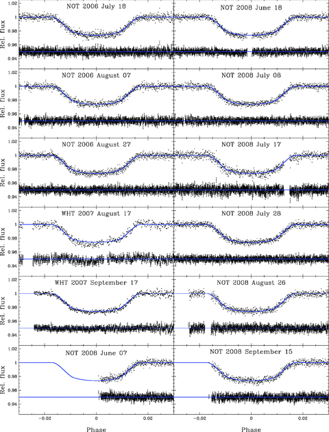
Differential photometry of the HD 189733 system overplotted with the best-fitting model (solid line) from the MCMC fit. The residuals and 1σ error bars are also plotted, offset by a constant flux for clarity. The phase was computed using best-fitting transit times presented in Table 1. The photometry for NOT data is unbinned and for WHT is binned in time with 10-s bins to give the similar cadence as for NOT data for clarity.

Open in new tabDownload slide

4 LIGHT-CURVE MODELLING

To estimate the system parameters, we used a parametrized model where we assumed a circular orbit around the centre of mass to calculate the normalized separation, z, of the planet and star centres as a function of time. The analytic formulas of Mandel & Agol (2002) were used to calculate the fraction of the stellar flux occulted by the planet using z and the planet-to-star radius ratio, ρ. We assumed a quadratic limb darkening law:

1

where I is the intensity, μ is the cosine of the angle between the line of sight and the normal to the stellar surface and u₁ and u₂ are the linear and quadratic limb-darkening coefficients. For the NOT data, we allowed the limb-darkening coefficients to be free parameters, in order to include possible errors in the limb-darkening coefficients into our final system parameters and mid-transit times. For the WHT data, we adopted values u₁= 0.4970 and u₂= 0.2195 from the tables of Claret (2000) and fixed them in the subsequent analysis. These correspond to the Johnson R filter which has similar characteristics as the Kitt Peak R filter used.

To compute our model, we folded all the NOT light curves of full transit except for the night of 2008 July 17 which displays obvious systematic changes during transit. In our photometry, we cannot easily distinguish spot effects from systematic instrumental errors; to do so would require the instrumental systematic noise to be much less than the predicted spot signatures. We fitted simultaneously planetary and stellar radius, R_p and R_★, respectively, the orbital inclination, i, two limb-darkening coefficients, u₁ and u₂, transit time, T_0,n, and additional two parameters for each night n– the out-of-transit flux, f_oot,n, and a time gradient, t_Grad,n. These two parameters were allowed to be free to account for any normalization errors in the data. For each change of R_★, the stellar mass, M_★, was recomputed using the scaling relation R_★∝M^1/3_★. We fixed the planetary mass value M_p= 1.15 ± 0.04 M_J (Bouchy et al. 2005), adopted a period P= 2.2185 7503 ± 0.000 000 37 d (Agol et al. 2009), and using Kepler's third law we updated the orbital semimajor axis for each choice of M_★.

We ran Markov Chain Monte Carlo (MCMC) simulations (Tegmark et al. 2004; Ford 2006; Holman et al. 2006) with the Metropolis–Hastings algorithm (Ford 2005) to estimate the best-fitting parameters and their uncertainties. From an initial point, a chain is generated by iterating a jump function, which adds a random value selected from a Gaussian distribution with mean 0 and a standard deviation 1, scaled by a factor specific for each parameter so that ∼44 per cent of each parameter sets are accepted (Gelman et al. 2003; Ford 2006). In each step of the generated chain, the χ²-fitting statistic for old and new parameter values is computed:

2

Here, f_i(obs) is the flux observed at time i, σ_i is the corresponding uncertainty, f_i(theor) is the flux calculated using formulas of Mandel & Agol (2002) and N_DOF is the number of degrees of freedom for each light curve. The new parameter is then accepted if its χ² is lower than that for the previous parameter, or accepted with a probability p= exp(−Δχ²/2) if its χ² is higher. The second term in equation (2) is a Gaussian prior placed on M_★, where M₀= 0.82 M_⊙ and is the stellar mass and its uncertainty, estimated from stellar spectra by Bouchy et al. (2005). This ensures that errors in the stellar mass, which are the greatest source of uncertainty when deriving the system parameters and transit times, are taken into account.

The scale factors were chosen so that ∼44 per cent of parameter sets were accepted (Gelman et al. 2003; Ford 2006). For each simulation, we created 10 independent chains, with length at least 100 000 points per chain to ensure convergence. Each chain was initiated by a parameter that was within ±5σ of a previously known best-fitting parameter value using the estimated uncertainty σ. The first 20 per cent of each chain was discarded to minimize the effect of the initial conditions. We checked convergence of generated chains using the Gelman & Rubin (1992)R statistic and created chains until R < 1.03, a good sign of convergence.

To estimate appropriate error bars in our data accounting for any correlated noise, we used a procedure similar to that of Gillon et al. (2006) and Narita et al. (2007). We assigned the same error bars to all the data points including only Poisson noise. An initial MCMC analysis of the folded NOT light curves was used to estimate the parameters R_p, R_★, i, u₁, u₂, T_0,n, f_oot,n and t_Grad,n. The first model light curve was used to find the differences between the data and the model for each individual night. Then, we rescaled the error bars to satisfy the condition χ²/N_DOF= 1.0. For the night of 2008 July 17, the nights of the two partial transits (2008 June 07 and 2008 September 15) and for the WHT light curves (2007 August 17 and 2007 September 17) we adopted our first model and ran MCMC analysis to find initial parameters T₀, f_oot and t_Grad for each night independently. Then, we rescaled the error bars similarly as before. We assume that our initial model is a good description of the light curve. Compared to this model, we found that for the NOT data errors are higher by factors of 2.3–3.4 than errors including only Poisson noise and for the WHT data by factors of 4.6 and 4.4 for the two nights, respectively. The data rms errors per exposure are presented in Table 1. The predicted rms due to photon noise, which is dominated by the fainter comparison star, and to atmospheric scintillation, is ∼2.5 mmag for the NOT data and ∼3 mmag for the WHT data.

The amplitude of systematic trends in the photometry was estimated from the standard deviation over one residual point, σ₁, and from the standard deviation of the average of the residuals over N successive points, σ_N. We solved the following system of two equations given by Gillon et al. (2006):

3

4

to obtain the amplitude of the white noise, σ_w, which is uncorrelated and averages down as (1/N)^1/2, and the red noise, σ_r, which is correlated and remains constant for specified N. The error bars were then adjusted by multiplying by [1 +N(σ_r/σ_w)²]^1/2 and these rescaled uncertainties were used for the subsequent fitting procedure. To account properly for the systematic errors, the resulting multiplying factor was computed as the average of values using different N in the range 15–30 min (the typical time-scale of ingress and egress).

To create our final model, we proceeded as before but this time including systematic noise in our data and therefore properly estimating parameter uncertainties. We ran MCMC using the folded NOT light curves and fitting the parameters as described earlier. We created 10 chains, each with length 2 000 000 points in order to achieve convergence. Ultimately, we used our final model to find individual mid-eclipse times and two normalization parameters for the night of 2008 July 17, the nights of the two partial transits (2008 June 07 and 2008 September 15) and for the WHT light curves (2007 August 17 and 2007 September 17).

5 RESULTS

The final system parameters are presented in Table 2 and are consistent within ∼2σ error bars with the previously published values (Bakos et al. 2006b; Pont et al. 2007; Winn et al. 2007; Miller-Ricci et al. 2008). The resulting limb-darkening coefficients for the NOT data were u₁= 0.46 ± 0.10 and u₂= 0.35 ± 0.13.

The final barycentric transit times can be found in Table 1. The uncertainties are defined as 68 per cent confidence limits. To compute the observed minus calculated values (O − C) we used the ephemeris given by Agol et al. (2009):

5

The resulting O − C residuals together with all the other previously published values (Bakos et al. 2006b; Pont et al. 2007; Winn et al. 2007; Miller-Ricci et al. 2008; Knutson et al. 2009) are plotted in Fig. 2. Our observations did not bring any refinement of the ephemeris and we confirm that presented by Agol et al. (2009). For the night of 2006 August 07, a transit timing measurement of HD 189733 was also presented by Miller-Ricci et al. (2008) from the MOST data and it is consistent within 2σ error bars with our measurement.

Figure 2

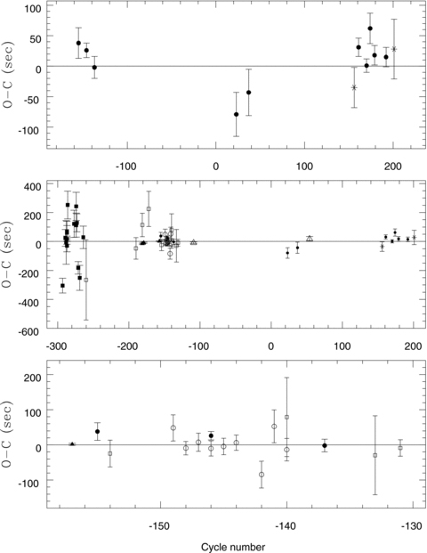
Top panel: NOT and WHT O − C residuals of mid-transit times of the HD 189733 system including both partial (star symbol) and full transits (filled circle symbol). Middle panel: previously published values plotted together with NOT and WHT results. Filled squares –Bakos et al. (2006b), ground based; filled triangles –Pont et al. (2007), HST; open squares –Winn et al. (2007), ground based; open circles –Miller-Ricci et al. (2008), MOST; open triangles –Knutson et al. (2009), Spitzer; filled circles and stars – this work. Bottom panel: the same as the middle but zoomed for clarity. The cycle number is in periods from the ephemeris given by Agol et al. (2009). A horizontal line is plotted in each panel at O − C = 0 to guide the eye. Our timing measurements are the most accurate from known ground-based observations.

Open in new tabDownload slide

5.1 Transit timing variations analysis

For all our observations which span more than 2 years, the mean O − C = 5 ± 38 s, where the quoted error is the rms scatter in the O − C values and is slightly larger than the average O − C uncertainty ∼25 s. None of our O − C measurements is a significant outlier. The two largest O − C values for the nights of 2007 August 17 and 2008 July 17 coincide with obvious systematic changes during the transit (see Fig. 1) and both have the same or larger uncertainty than the average value. Therefore, the rms scatter in the O − C values of 38 s is a good estimate for placing limits on the presence of other planets in the system.

We used this conclusion to place mass limits on the existence of planets on orbits interior and exterior to HD 189733b. First, we selected the mass, semimajor axis and eccentricity of the putative perturbing planet. The orbital inclination was set so that HD 189733b and the perturbing planet have coplanar orbits. The two-planet system was then numerically integrated using the Bulirsch–Stoer integrator (Press et al. 1992). We determined all mid-transit times of HD 189733b over a time-span of 500 days, an interval long enough to cover at least 14 orbits of all perturbing planets we can exclude, and used these data to estimate TTVs. The mass, initial semimajor axis and initial eccentricity of the perturbing planet were varied to determine the TTV amplitude for different planetary configurations.

Fig. 3 shows the range of the inner and outer planet's orbits that produce TTVs smaller/larger than ±38 s and are thus compatible/incompatible with our TTV observations of the HD 189733 system. The shaded area in Fig. 3 excludes a range of possible eccentricities and semimajor axes for a putative 1 Earth-mass (top plots) and 2 Earth-masses (bottom plots) inner (left-hand plots) and outer (right plots) planet in the system. Based on this analysis, our observations of the HD 189733 system show no evidence for the presence of planets down to 1 Earth mass in the 2:1, 3:2 and 5:3 exterior resonance orbits, planets down to 1 Earth mass in the 1:2, 1:3, 2:3 and 2:5 interior resonance orbits and planets down to 2 Earth masses in the 1:4 interior resonance orbit with HD 189733b. However, not all of these resonant orbits are Hill stable. We computed the Hill stability according to equation (21) of Gladman (1993) for both inner and outer perturbing planet and displayed the result in Fig. 3 using thin solid line. For the inner/outer perturbing planet, all the orbits on the left/right to the thin solid line are Hill stable, which means that close approaches between two planets are forbidden. For the rest of the parameter space the Hill stability of the system is unknown; the system still may be Hill stable.

Figure 3

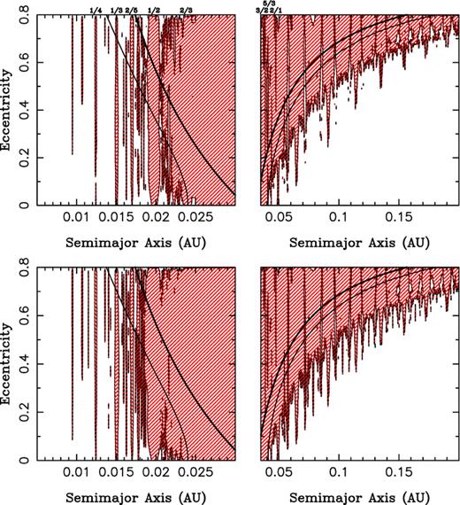
A numerical survey of the HD 189733 system showing 38-s TTVs caused by an inner (left-hand plots) and outer (right-hand plots) 1 Earth-mass planet (m₂= 3 × 10⁻⁶ M_⊙, top plots) and 2 Earth-mass planet (m₂= 6 × 10⁻⁶ M_⊙, bottom plots). The shaded area excludes a range of possible eccentricities and semimajor axes for a putative 1 and 2 Earth-mass inner/outer planet in the system based on our observational non-detection of TTVs greater than ±38 s. We do not display plots for Jupiter-mass planets as these would easily be detected in radial velocity searches. The thick solid line shows a boundary where a collision between the two planets can occur. It is defined so that the apocentre/pericentre of the inner/outer perturbing planet equals to the semimajor axis of the transiting planet. The thin solid line represents a Hill stability computed according to Gladman (1993). On the top of the upper panel, we indicate the major resonances of the putative perturbing planet and HD 189733b.

Open in new tabDownload slide

Nesvorný (2009) showed that the TTV signal can be significantly amplified for planetary systems with substantial orbital inclinations of the transiting and perturbing planet and/or in the case of transiting planet in an eccentric orbit with an anti-aligned orbit of the perturbing planetary companion. Therefore, for most orbital architectures of exoplanetary systems we determine the perturber's upper mass from our TTVs under the assumption of coplanar orbits of transiting and perturbing planets.

However, the above-mentioned analysis does not take into account time sampling of our measured transit times and their uncertainties. It is possible to have a system whose TTV amplitude exceeds 38 s but remains consistent with the available transit timing data. To assure that the limits on additional planets presented in this paper are not overestimated, in addition to our previous analysis we compared model timing residuals against the transit times to place upper mass limits for a putative perturbing planet. We used the same procedure as Gibson et al. (2009, 2010), where more details can be found. To compute model timing residuals, we integrated the equations of motion for a three-body system using a fourth-order Runge–Kutta method, with the first two bodies representing the star and planet of the HD 189733 system and the third body representing a putative perturbing planet. The transit times were extracted when the star and transiting planet were aligned along the direction of observation, and the residuals from a linear fit were taken to be the model timing residuals. For each model, TTVs were extracted for six equally spaced directions of observations, and we simulated 3 years of TTVs to cover the full range of observations. The resulting TTVs were then compared to transit times presented in the middle panel of Fig. 2, i.e. all available transit times. Due to computational limitations, we assumed that the amplitude of the timing residuals scales proportionally to the perturber mass (Agol et al. 2005; Holman & Murray 2005), a perturber has circular orbit and the orbits of the planets are coplanar.

We created models with period ratios in the range 0.2–5.0, increasing the sampling around the interior 1:2 and exterior 2:1 resonances. The maximum allowed mass for each model was calculated as in Gibson et al. (2009, 2010). We scaled the perturber mass until the χ² of the model fit increased by a value Δχ²= 9 (Steffen & Agol 2005) from that of a linear ephemeris. Then, we minimized the χ² along the epoch, and rescaled the perturber mass again until the maximum allowed mass was determined. This was repeated for each direction of the observation, and the maximum mass found was set as our upper mass limit. This process was repeated twice to verify our assumption that the timing residuals scale proportionally with the mass of the perturbing planet.

The resulting upper mass limits are plotted as a function of the period ratio in Fig. 4. The solid line represents the upper mass limits from our three-body simulations, and the horizontal dashed line shows an Earth-mass planet. Based on this analysis, the available data were sufficiently sensitive to probe for masses as small as 0.2 and 0.15 M_⊕ near the interior 1:2 and exterior 2:1 resonances with HD 189733b, respectively. The corresponding upper masses near the 3:5 and 5:3 resonances with HD 189733b are 2.2 and 0.54 M_⊕. In the rest of the space outside the region between the 2:3 and 3:2 resonances with HD 189733b, the upper mass limits are of the order of a few tens of Earth masses to a few Jupiter masses. However, these upper mass limits result from the assumption of a circular orbit of a perturber. Eccentric orbits may lead to smaller TTVs, and hence planets larger than our upper mass limits in eccentric orbits could exist in these regions. Unfortunately, accounting for eccentric orbits is computationally unfeasible using these models due to a large parameter space. Thus, real upper mass limits of a perturber in a low-eccentric orbit can be as much as an order of magnitude larger (Gibson et al. 2010).

Figure 4

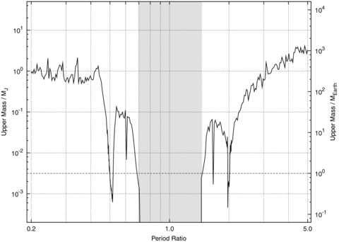
Upper mass limits on a putative second planet in the HD 189733 system as a function of period ratio based on the comparison of model timing residuals and all available transit times. The solid line represents the upper mass found using three-body simulations. The horizontal dashed line shows an Earth-mass planet. The grey area is the region where an Earth-mass perturbing planet is not guaranteed to be Hill stable.

Open in new tabDownload slide

We also consider the possible presence of Trojans in the system. According to Ford & Holman (2007), transit times are the same for a system without a Trojan and for a system where the transiting planet and Trojan have equal eccentricities and the Trojan resides exactly at the Lagrange L4/L5 fixed point. TTV analysis alone is not suitable for constraining the presence of Trojans in transiting systems. However, a comparison of the photometrically observed transit time and the transit time calculated from the radial velocity data assuming zero Trojan mass can reveal a Trojan or place upper limits on its mass. Such an analysis was performed by Madhusudhan & Winn (2009) who found an upper limit of 22 M_⊕ for a Trojan in the HD 189733 system. In addition, Croll et al. (2007) searched for Trojan transits in MOST photometry, assuming similar inclinations of the Trojan's and transiting planet's orbits, and concluded that Trojans with a radius above 2.7 R_⊕ should have been detected with 95 per cent confidence. Using a mean density of ρ∼ 3000 kg m⁻³, this corresponds to 11 M_⊕. We used equation (1) of Ford & Holman (2007) to estimate what Trojan's mass can be excluded in the system based on 38-s rms of our TTVs. However, the amplitude of the angular displacement of a putative Trojan from the Langrange point is not known. If these libration amplitudes are similar as for Trojans orbiting near the Sun–Jupiter Langrange points, that is 5°–30° (Murray & Dermott 2000), our TTVs show no evidence for Trojans with masses higher than 5.3 M_⊕.

For an Earth-mass exomoon in a circular orbit about HD 189733b, Kipping (2009) predicted TTV amplitude of 1.51 s and transit duration variation (TDV) amplitude of 2.94 s. Increasing the eccentricity of the moon's orbit decreases TTV amplitude, but increases TDV amplitude. However, for the HD 189733 system these variations are too small to be detectable in our data.

6 CONCLUSIONS AND DISCUSSION

Miller-Ricci et al. (2008) found no TTVs greater than ±45 s in MOST data, and excluded super-Earths of masses larger than 1 and 4 M_⊕ in the 2:3 and 1:2 inner resonance, respectively, and planets greater than 20 M_⊕ in the outer 2:1 resonance of the known planet and greater than 8 M_⊕ in the 3:2 resonance. Miller-Ricci et al. (2008) assumed that the orbit of the perturbing planet is circular and that additional planets in eccentric orbits would produce stronger perturbations. However, Nesvorný (2009) showed that an eccentric planet can produce stronger or weaker perturbations depending on the relative angular position of its orbital pericentre.

In this paper, we used two different methods to determine the upper mass limits for a putative perturbing planet in the HD 189733 system and thus the results of both analyses can be directly compared. Our first analysis does not take into account time sampling of the measured transit times and their uncertainties. On the other hand, it was possible to probe for eccentric orbits of a perturbing planet, which is more rigorous than assuming a circular orbit (Nesvorný 2009). Further analysis was performed to assure that the limits on additional planets presented in this paper are not overestimated. Unfortunately, applying this method for eccentric orbits of a perturbing planet would increase the number of parameters enormously, thus we assumed a circular orbit for the perturber.

Due to the limitations of our TTV analyses, we adopt the least constraining limits to conclude what upper masses of a putative perturbing planet can be excluded in the HD 189733 system. The results show no evidence for the presence of planets down to 1 Earth mass near the 1:2 and 2:1 resonance orbits, and planets down to 2.2 Earth masses near the 3:5 and 5:3 resonance orbits with HD 189733b. These are the strongest limits to date on the presence of other planets in this system, based on results of two independent TTVs analyses. We also discuss the possible presence of Trojans in the system, and conclude that the highest limit on a Trojan mass is 5.3 M_⊕ if its libration amplitude is similar as for Trojans orbiting near the Sun–Jupiter Lagrange points.

We would like to thank the anonymous referee for useful suggestions and improvements. We are grateful to P. Harmanec and R. Karjalainen for their careful reading of the manuscript and comments. The data presented here have been taken using ALFOSC, which is owned by the Instituto de Astrofisica de Andalucia (IAA) and operated at the NOT under agreement between IAA and the NBIfAFG of the Astronomical Observatory of Copenhagen. The research was supported by the grants 205/08/H005 and 205/06/0304 of the Czech Science Foundation, from the Research Program MSM0021620860 of the Ministry of Education of the Czech Republic and by the DFG grant HA 3279/5-1. We acknowledge the use of the electronic bibliography maintained by NASA/ADS system and by the CDS in Strasbourg.

REFERENCES

Author notes