Second-order Lagrangian perturbation theory initial conditions for resimulations

Abstract

1 INTRODUCTION

Computer simulations of cosmological structure formation have been crucial to understanding structure formation particularly in the non-linear regime. Early simulations e.g. Aarseth, Turner & Gott (1979) used only around a thousand particles to model a large region of the Universe, while recent simulations of structure formation have modelled over a billion particles in just a single virialized object (Springel et al. 2008; Stadel et al. 2009). Since the advent of the cold dark matter (CDM) model (Peebles 1982; Davis et al. 1985), most computational effort has been expended modelling structure formation in CDM universes. Early work in the 1980s focused on ‘cosmological’ simulations where a representative region of the universe is modelled, suitable for studying large-scale structure (Davis et al. 1985). The starting point for these CDM simulations, the initial conditions, are Gaussian random fields. The numerical techniques needed to create the initial conditions for cosmological simulations were developed in the 1980s and are described in Efstathiou et al. (1985).

As the algorithms for N-body simulations have improved, and the speed of computers increased exponentially with time, it became feasible in the 1990s to simulate the formation of single virialized haloes in the CDM model with enough particles to be able to probe their internal structure (e.g. Navarro, Frenk & White 1996, 1997; Ghigna et al. 1998; Moore et al. 1999). These more focused simulations required new methods for generating the initial conditions. The algorithm of Hoffman & Ribak (1991) for setting up constrained Gaussian random fields was one method which could be applied to setting up initial conditions for a rare peak where a halo would be expected to form. The essence of this technique is that it allows selection of a region based on the properties of the linear density field. However, the objects we actually observe in the Universe are the end products of non-linear structure formation and it is desirable, if we want to understand how the structure we see formed, to be able to select objects on the basis of their final properties.

This requirement led to an alternative method for producing initial conditions based first on selecting objects from a completed simulation (e.g. Katz et al. 1994; Navarro & White 1994). The initial conditions for the first or parent simulation were created using the methods outlined by Efstathiou et al. (1985). The density field is created out of a superposition of plane waves with random phases. Having selected an object at the final (or any intermediate) time from the parent simulation, a fresh set of initial conditions with higher numerical resolution in the region of interest, which we will call ‘resimulation’ initial conditions (also called ‘zoom’ initial conditions), can be made. Particles of different masses are laid down to approximate a uniform mass distribution, with the smallest mass particles being concentrated in the region from which the object forms. The new initial conditions are made by recreating the same plane waves as were present in parent simulation together with the addition of new shorter wavelength power.

An alternative technique for creating resimulation initial conditions was devised by Bertschinger (2001) based on earlier work by Salmon (1996) and Pen (1997) where a Gaussian random field with a particular power spectrum is created starting from a white noise field. Recently, parallel code versions using this method have been developed to generate very large initial conditions (Prunet et al. 2008; Stadel et al. 2009). A feature common to both these techniques, to date, is that the displacements and velocities are set using the Zel'dovich approximation (Zel'dovich 1970), where the displacements scale linearly with the linear growth factor.

It has long been known that simulations starting from Zel'dovich initial conditions exhibit transients and that care must be taken choosing a sufficiently high start redshift so that these transients can decay to a negligible amplitude (e.g. Efstathiou et al. 1985). A study of the behaviour of transients using Lagrangian perturbation theory by Scoccimarro (1998) showed that for initial conditions based on the second-order Lagrangian perturbation theory (2lpt) the transients are both smaller and decay more rapidly than first-order, or Zel'dovich, initial conditions. Scoccimarro (1998) gave a practical method for implementing second-order Lagrangian initial conditions. The method has been implemented in codes for creating cosmological initial conditions by Sirko (2005) and Crocce, Pueblas & Scoccimarro (2006). These codes are suitable for making initial conditions for cosmological simulations, targeted at large-scale structure, but they do not allow the creation of resimulation initial conditions, the focus of much current work on structure formation.

In this paper, we describe a new method for creating second-order Lagrangian initial conditions which can be used to make resimulation initial conditions. The paper is organized as follows: in Section 2, we introduce 2lpt initial conditions and motivate their advantages for studying structure in the non-linear regime by applying them to the spherical top-hat model; in Section 3, we describe how Zel'dovich resimulation initial conditions are made, and the new method for creating 2lpt initial conditions, and test the method against an analytic solution for a spherically symmetric perturbation; in Section 4, we apply the method and analyse the formation of a dark matter halo at high and low redshifts for varying starting redshifts for both Zel'dovich and 2lpt initial conditions; in Section 5, we summarize and discuss the main results and in the appendix we evaluate two alternate interpolation schemes which have been used in the process of making resimulation initial conditions.

2 THE MOTIVATION FOR USING SECOND-ORDER LAGRANGIAN PERTURBATION THEORY INITIAL CONDITIONS

In this section, we give a brief summary of Lagrangian perturbation theory (Section 2.1), concentrating on the second-order approximation, and illustrate the difference they make for the spherical top-hat model in Section 2.2. The method we describe could be developed further to create third-order Lagrangian perturbation initial conditions. However, Scoccimarro (1998) concluded that the gains from going from second to third order were relatively modest while the complexity of computing the third-order terms is considerable.

2.1 Summary of second-order Lagrangian perturbation theory

We give only a bare-bones account of second-order perturbation theory here. Detailed discussions of Lagrangian perturbation theory in general can be found in the literature (e.g. Buchert 1994; Buchert, Melott & Weiss 1994; Bouchet et al. 1995; Scoccimarro 1998). We follow the notation used in appendix D1 of Scoccimarro (1998).

In Lagrangian perturbation theory, the Eulerian final comoving positions x are related to the initial positions q via a displacement field, Ψ(q):

1

It can be shown for 2lpt that the displacement field is given, in terms of two potentials φ⁽¹⁾ and φ⁽²⁾, by

2

where D₁ is the linear growth factor and D₂ is the second-order growth factor, which is given by D₂≈−3D²₁/7. The subscripts q refer to partial derivatives with respect to the Lagrangian coordinates q. Similarly, the particle comoving velocities v are given to second order by

3

where H is the Hubble constant, the f_i= d ln D_i/d ln a (a is the expansion factor). For flat models with a non-zero cosmological constant, the following relations apply f₁≈Ω^5/9, f₂≈ 2Ω^6/11 (Bouchet et al. 1995), where Ω is the matter density. In practice, these approximations for f₁, f₂ and D₂ are extremely accurate when applied to making most actual ΛCDM initial conditions, as the start redshift is high enough that Ω is very close to unity.

The potentials φ⁽¹⁾ and φ⁽²⁾ are obtained by solving a pair of Poisson equations:

4

where δ¹⁾ (q) is the linear overdensity, and

5

We will refer to the term δ⁽²⁾ (q), as the ‘second-order overdensity’. In fact, this quantity is related to the linear overdensity field by the following quadratic expression:

6

where we use φ,_ij≡∂²φ/∂q_i∂q_j for short.

The most common technique used in making cosmological initial conditions, to date, is the Zel'dovich approximation (Zel'dovich 1970). Zel'dovich initial conditions can equivalently be called first-order Lagrangian initial conditions, and are given by ignoring the terms with φ⁽²⁾ in equations (2) and (3). A variant of Zel'dovich initial conditions was advocated by Efstathiou et al. (1985). In this case, the velocities are not set proportional to the displacements, but proportional to the gravitational force evaluated for the displaced particle distribution. This method for setting the velocities gives weaker transients, as discussed in Scoccimarro (1998), although the scaling of the transients with redshift is unaffected. In this paper, we use the term Zel'dovich initial conditions to mean the velocities are proportional to the displacements. We note, and we will exploit the fact later, that the individual terms on the right-hand side of equation (6) are the derivatives of the first-order Zel'dovich displacements which are linear in the potential φ⁽¹⁾.

2.2 The spherical top-hat model

The spherical top-hat model (Peebles 1980) provides a convenient way to illustrate the relative merits of Zel'dovich and 2lpt initial conditions. Apart from the significant advantage of mathematical convenience, there are other reasons for considering this special case.

• The first collapsed structures in a cosmological simulation will form from the regions with the highest linear overdensity. In the limit of high peak height, the regions around the maxima in a smoothed linear overdensity field become spherical (Bardeen et al. 1986). As we will see, it is the first structures which are most sensitive to whether the initial conditions are Zel'dovich or 2lpt.

• It is easy to show that the second-order overdensity, δ⁽²⁾, is related to the first-order overdensity, δ⁽¹⁾, through the inequality: ⁠, with equality occurring for isotropic compression or expansion. For a fixed linear overdensity, the second-order overdensity is maximized for isotropic compression, so the spherical top hat is the limiting case where the affects of second-order initial conditions are maximized.

For convenience, we will consider, for now, the top-hat in an Einstein–de Sitter universe. In this case, the spherical top-hat solution is most elegantly expressed in a parametric form as follows. For an overdense spherical top hat which begins expanding at t= 0 and reaches a maximum physical radius of expansion, R₀, and collapses back to zero radius at time, t_c, the parametric solution is

7

where 0 ≤η≤ 2π. These equations can be derived by solving the equation of motion for the top hat:

8

and applying the appropriate boundary conditions.

If we were to solve the spherical top-hat problem instead by the techniques used in cosmological numerical simulations, we would begin by creating initial conditions consisting of a set of particles with given masses, positions and velocities, at a time, t, soon after the start of the expansion. The solution would be obtained by evaluating the gravitational interactions between the particles and integrating the equations of motion of all the particles forward in time. For a real simulation, the accuracy of the subsequent solution would depend not only on the accuracy of the initial conditions but also on numerical aspects such as the time-integration scheme and the force accuracy. For our purposes, we will assume that these numerical sources of error can be overcome, and will only consider the effects of using either Zel'dovich or 2lpt initial conditions on the subsequent evolution of the top-hat.

The Zel'dovich and 2lpt initial conditions needed to start a cosmological simulation of a top-hat are most easily obtained using the rather less elegant power series representation of the spherical top-hat solution. The power series in t corresponding to equation (7) is

9

and the corresponding velocity, ⁠, is

10

The leading order term in equation (9) represents the expansion of a perturbation with mean cosmic density which grows in time in the same way as the scalefactor for an Einstein-de Sitter universe. The second to leading term gives the linear growth of an overdense spherical growing mode perturbation and it is easy to verify from equation (9) that the linear overdensity at t=t_c, when the non-linear solution collapses to a point, is given by δ_c= 3(12π)^2/3/20 ≃ 1.686, familiar from the Press–Schechter theory (Press & Schechter 1974).

We obtain the Zel'dovich initial condition for the spherical top-hat by taking just the first two leading terms in r and in equations (9) and (10). The equivalent 2lpt initial conditions correspond to taking the first three terms instead. We can follow the top-hat solution starting from these initial conditions, up until the point when the sphere collapses to zero radius, by integrating the equation of motion equation (8) forward in time from time, t, using the values of r and at time t as the boundary conditions.

In Fig. 1, the black solid line shows the parametric top-hat solution given by equation (7). The red solid curve shows a spherical top-hat model integrated forward from the arbitrarily chosen time, t=t_c/27, starting from the Zel'dovich initial condition (marked with a red dot). The cyan dashed curve shows the corresponding result starting with the 2lpt initial condition at t=t_c/27. The solution using the 2lpt initial condition is very much closer to the analytic solution than the curve started from the Zel'dovich initial condition.

Figure 1

Evolution of a top-hat spherical perturbation. The black curve shows the radius of a spherical top-hat perturbation as a function of time for an Einstein-de Sitter universe. The analytic solution starts expanding at t= 0 and collapses at a time t=t_c and has a maximum physical radius of expansion of R₀. The red and dashed cyan curves show the spherical top-hat solution obtained by integrating the equation of motion for the top-hat starting from t=t_c/27 and, respectively, initializing the radius and its velocity with the Zel'dovich and 2lpt initial condition. The result for the 2lpt initial condition is more accurate than for the Zel'dovich initial condition where the time of collapse is significantly delayed.

Open in new tabDownload slide

The collapse time for the top-hat for both the Zel'dovich and 2lpt initial conditions occurs later than the analytic solution. This delay, or timing error, Δt, can be quantified as follows. Multiplying equation (8) by and integrating gives an integral of the motion: For the analytic solution, this can easily be evaluated at the radius of maximum expansion which gives E=−π²R²₀/2t²_c. The corresponding values of E for the Zel'dovich and 2lpt solutions can be obtained by substituting the first two or three terms, respectively, from equations (9) and (10) into the expression for E. The expansion time, t_c, of the top-hat over the complete cycle, by analogy with Keplerian orbits, is related to E by d ln t_c/d ln |E| =−2/3 for bound motion in an Einstein-de Sitter universe. We can generalize this result to flat universes with a cosmological constant by numerically integrating equation (8) with an added term for the cosmological constant. In this case, we find, by fitting to the results of numerical integration, an equivalent approximate relation: ⁠, valid to an fractional accuracy of less than 1.2 per cent for 0.25 < Ω_c≤ 1, where Ω_c is the matter density in units of the critical density at the time of collapse, provided t_s≪t_c so the cosmological constant is negligible at t_s.

Knowing d ln t_c/d ln|E| and assuming again the condition that the starting time of the initial condition, t_s, obeys, t_s≪t_c, allows the fractional timing error, Δt/t_c, to be obtained, to leading order in t_s/t_c, for both types of initial condition, from the ratio of E for the analytic solution, respectively, with the value of E for Zel'dovich or 2lpt initial conditions.

Applying these results we find after some algebra that the timing error for Zel'dovich initial conditions to lowest order is

11

Similarly, the 2lpt initial condition fractional timing error is given by

12

Alternatively, these results can be expressed in terms of the start redshift of a numerical simulation, z_s. Relative to an analytic spherical top-hat with collapse occurring at redshift, z_c, where z_c≪z_s, the fractional timing error is given for Zel'dovich initial conditions by

13

and for 2lpt initial conditions it is

14

where we have made use another approximate relation: t^2/3(1 +z) ∝Ω^0.13 relating redshift, z, to the age of the universe, t, and the value of Ω all at time t, which is accurate to better than 1 per cent in the range 0.25 < Ω≤ 1 for a flat universe with a cosmological constant.

Ignoring the weak Ω dependence, the timing error for the 2lpt initial condition shows a quadratic scaling with the ratio of the expansion factor at the start to that at the time of collapse, while for Zel'dovich initial conditions the scaling is just linear. These results for spherical collapse are consistent with the more general behaviour of the decay of transients discussed in Scoccimarro (1998). The absolute value of the timing error, Δt, for a fixed start redshift, actually decreases with increasing collapse time for 2lpt initial conditions. For Zel'dovich initial conditions, the timing error grows slowly with increasing collapse time. However, by starting at sufficiently high redshift, the timing error for the Zel'dovich initial conditions can be made small. It is common practice to start simulations from Zel'dovich initial conditions at a high redshift for this reason so that the transients have sufficient time to decay to a negligible amplitude.

Equating the fractional timing errors for equations (13) and (14) gives an objective way of defining an equivalent starting redshift for Zel'dovich or 2lpt initial conditions for a given choice of collapse redshift. To be conservative, it would be natural to choose the collapse redshift to be the first output redshift of the simulation which is of scientific interest. To give a concrete example, ignoring the Ω dependence, if the 2lpt initial conditions are created a factor of 10 in expansion before the first output, the equivalent Zel'dovich initial conditions would need to start at a factor of about 160 in expansion before the first output. Using 2lpt initial conditions instead of Zel'dovich initial conditions can therefore lead to a significant reduction in computer time because the simulations can be started later. A later start has further advantages as force errors, errors due to the discreteness in the mass distribution and time integration errors all accumulate as the ratio of the final expansion factor to the initial expansion factor increases. All of these reasons make 2lpt initial conditions attractive for the simulator. In the next section, we describe the new method to make 2lpt initial conditions.

3 MAKING SECOND-ORDER LAGRANGIAN RESIMULATION INITIAL CONDITIONS

In this section, we explain what resimulation initial conditions are and describe how they can be made. We will describe the method currently in use to make initial conditions for the Virgo Consortium for Supercomputer Simulations.1 The Virgo resimulation code to date generates Zel'dovich initial conditions. In Section 3.1, we describe the process for making these Zel'dovich resimulation initial conditions. In Section 3.2, we describe the new method to generate 2lpt initial conditions. In Section 3.3, we demonstrate by comparing with an analytic solution that the method works in practice.

3.1 Setting up Zel'dovich resimulation initial conditions

The current method used by the Virgo code is based on the ideas first described in Navarro & White (1994). The actual implementation has changed considerably over time with increasingly up-to-date accounts being given in Power et al. (2003), Navarro et al. (2004) and Springel et al. (2008).

The need for resimulation initial conditions stems from the desire to repeat a particular simulation of structure formation with (usually) higher mass resolution in one or more regions than was present in the original, or parent, simulation. The parent simulation may have been run starting from cosmological initial conditions or it may be a resimulation itself. The following list gives the steps needed to create a set of resimulation initial conditions from a parent simulation.

• Identify the region(s) of interest in the parent simulation where higher mass resolution is required.

• Create a force-free multimass particle distribution which adequately samples the high-resolution region(s) of interest identified in (i) with low-mass particles. This particle distribution needs to be a good approximation to an isotropic and homogeneous mass distribution. The initial density fluctuations are created by perturbing the positions and assigning velocities to each of the particles. The region exterior to the high-resolution region can often be sampled more crudely than the parent simulation, using larger mass particles, as its only purpose is to ensure that the gravitational tidal field in the high-resolution region is accurately reproduced. Typically, the masses in the exterior region scale roughly as the cube of the distance from the high-resolution region. We will refer to this special particle distribution from now on as the ‘particle load’.

• Recreate the displacement and velocity fields for the parent simulation and apply the displacements and assign the velocities to the particle load created in (ii).

• Add extra small-scale fluctuations to the region of interest only, to account for the fact that the mass distribution in the resimulation is now more finely sampled than the parent simulation and therefore has a higher spatial Nyquist frequency. For Zel'dovich initial conditions, this high spatial frequency power can be added linearly to the low-frequency power copied from the parent simulation.

In this paper, we will not be concerned with steps (i) and (ii), which are common to resimulations in general, but will concentrate on adapting steps (iii) and (iv) to allow the creation of 2lpt initial conditions.

The displacement and velocity fields needed to perturb the particle load can in practice be efficiently created using Fourier methods. Adopting periodic boundary conditions when setting up the perturbations forces the Fourier representation of the density, displacement and velocity fields to be composed of discrete modes in the Fourier space. The amplitudes and phases of these modes are set as described in Efstathiou et al. (1985) to create a Gaussian random field with the appropriate power spectrum in Fourier space. Starting from the Fourier representation of the density field, it is straightforward to use discrete Fourier transforms to generate each of the components of the displacement field in real space. The discrete Fourier transform gives the displacements on a cubic lattice.

In practice, because computer memory is limited, more than one Fourier grid is required to be able to complete step (iv). These grids have different physical sizes, with the largest grid covering the entire periodic cubic volume, as is the case when making cosmological initial conditions. The additional grid(s) are given a smaller physical size, which means even with limited computer memory that they can generate a displacement field with power at higher wavenumbers than the largest grid, but only over a restricted part of the simulation volume. By nesting sufficient Fourier grids about the high-resolution region, it is possible to generate power all the way down to the particle Nyquist frequency in the high-resolution region. A description of the creation of the initial conditions for the Aquarius haloes, which required two Fourier grids, is given in Springel et al. (2008).

For Zel'dovich initial conditions, the displacement field at any location is formed by co-adding the displacement contributions from the one or more of these overlapping cubic Fourier grids, and the corresponding velocity field is simply proportional to the displacement field. For each Fourier grid, only a subset of the possible modes are assigned non-zero values. In k-space, these ‘populated’ modes are split between the different grids in a nested fashion around the origin. Each grid populates a disjoint region of k-space concentric on the origin, and taken together the modes from all the grids fill a spherical region in k-space around the origin. The smallest physical grid, which typically fits around just the high-resolution region, is used to represent the highest wavenumber modes in k-space. The highest wavenumber possible is limited by the particle Nyquist frequency which is determined by the interparticle separation.

A displacement field is generated on each Fourier grid. The complete displacement field is calculated by adding the contributions from the various grids together. To do this, it is necessary to define a set of common positions at which to co-add the displacements. The most natural common positions to use are those of the particle load itself, as the displacements need to be known at these locations to generate the Zel'dovich initial conditions. The displacements at the particle positions are computed by interpolating the values from the nearest Fourier grid points. A discussion of the interpolation methods currently in use and their associated errors is given for completeness in the appendix. The interpolation errors only become significant for fluctuations with a wavelength comparable to the Nyquist wavelength of the Fourier grid.

For the high-resolution region a second scale, the particle Nyquist wavelength also becomes important. Even in the absence of interpolation errors, the discreteness of the mass distribution affects the growth of linear fluctuations with wavelengths close to the particle Nyquist frequency (Joyce et al. 2005). We will not be concerned about either of these sources of error in the main part of the paper.

3.2 Generating 2lpt resimulation initial conditions

In Section 3.1, we outlined a method for making Zel'dovich initial conditions for resimulations. In this section, we will take this method for granted, and concentrate on how to augment the Zel'dovich initial conditions to produce 2lpt initial conditions. This is achieved, as can be seen from equations (2) and (3), by computing the components of the field ∇_qφ⁽²⁾. The second-order corrections to the Zel'dovich initial conditions for both the positions and the velocities are proportional to this quantity.

The second-order potential, ∇_qφ⁽²⁾, is obtained by solving the Poisson equation (5), where the source term is the second-order density field, δ⁽²⁾, given by equation (6). The right-hand side of this equation is a non-linear combination of six distinct terms, each of which is a second derivative of the first-order potential, φ⁽¹⁾. This same first-order potential is used to generate the Zel'dovich displacements and velocities. For this reason, as pointed out by Scoccimarro (1998), the calculation of the second-order overdensity field fits in very well with the generation of Zel'dovich resimulation initial conditions, from a computational point of view. The six second derivatives can be calculated using Fourier methods in the same way as is used to compute the first derivatives of φ⁽¹⁾ needed for the Zel'dovich approximation.

For initial conditions that can be made using a single Fourier grid, the six derivatives can be combined to give the value of δ⁽²⁾ at each Fourier grid point. The Poisson equation (5) can then be solved immediately using standard Fourier methods (Hockney & Eastwood 1988) to give the components of ∇_qφ⁽²⁾ at the grid points. Choosing a suitable cubic grid arrangement for the particle load ensures that the Lagrangian positions of the particles coincide exactly with Fourier grid points. This means the particle 2lpt displacements and velocities can be evaluated without the need for any spatial interpolation. This is the approach adopted by the 2lpt codes made available Sirko (2005) and Crocce et al. (2006).

The approach just described does not work when more than Fourier grid is used to generate the Zel'dovich initial conditions, because δ⁽²⁾ is a non-linear function of the first-order potential, φ⁽¹⁾, unlike the Zel'dovich displacements and velocities which are linear functions. The solution to this problem is simply to compute all six of the derivatives, which are linear functions of φ⁽¹⁾, for each Fourier grid, and co-add them. Then once the summation is complete for all six derivatives for a given position, compute δ⁽²⁾ using equation (6).

As with the Zel'dovich displacements, the values of the six derivatives need to be interpolated to a common set of positions before they can be co-added. It proves convenient again to use the particle load to define these common positions. Computationally, this entails storing six additional quantities per particle in computer memory. We use the quadratic interpolation (QI) scheme, described in the appendix, to interpolate the derivatives to the positions given by the particle load, as this scheme helps to minimize the interpolation errors, given limited computer memory. We have implemented the algorithm to compute δ⁽²⁾ for each particle in the particle load in a fortran/c code called ic_2lpt_gen. This code also computes the Zel'dovich displacements and velocities for each particle at the same time.

The final stage to make the 2lpt resimulation initial conditions is to solve the Poisson equation (5). At this point, it is no longer trivial to solve the equation by Fourier methods because the second-order overdensity field is known only at the positions of the particle load, which do not in general form a regular grid. However, it is relatively simple to solve the Poisson equation using an N-body code Poisson solver. It is natural, given that the purpose of creating the initial conditions in the first place is to integrate them forward in time with an N-body code, to use the same N-body code to solve both equation (5) and to integrate the equations of motion.

As mentioned in Section 3.1, in point (ii), the Lagrangian positions of the particle making up the particle load are special. The particles are distributed so that the mass density field is an excellent approximation to a uniform mass density, on scales larger than the interparticle separation. Furthermore, the gravitational force on any particle due to the others cancels out to a very good approximation. We can exploit the properties of the particle load in a simple way to reconstruct the second-order density field. To do this, we create a ‘2lpt particle load’ by taking the positions from the particle load, but replacing the particle masses with a ‘2lpt’ mass, given by

15

where λ is a constant numerical factor, whose value for now we will take to be unity.

With minimal modification, an N-body code can then be used to compute the gravitational force due to the 2lpt particle load acting on itself. By construction, this amounts to solving equation (5), with the resulting gravitational acceleration giving ∇_qφ⁽²⁾, at the positions given by the particle load. Provided the N-body code also reads in the Zel'dovich velocities for the particle load, the 2lpt initial condition positions and velocities can be evaluated using equations (2) and (3), respectively. Discarding the 2lpt masses and replacing them with the true particle masses completes the creation of the 2lpt resimulation initial conditions. The N-body code can then be used in the normal way to integrate the equations of motion for all of the particles.

The amplitude of the second-order overdensity field, and similarly ∇_qφ⁽²⁾, depends on the redshift of the initial conditions. By introducing the scaling factor λ into the ‘2lpt’ masses, and rescaling the resulting ∇_qφ⁽²⁾ by 1/λ to compensate, it is possible to make the calculation performed by the N-body code independent of the requested redshift of the initial conditions. It is desirable to implement this scaling if one wants to calculate ∇_qφ⁽²⁾ accurately for high-redshift initial conditions, as otherwise the inevitable force errors from the N-body force calculation will begin to dominate over the small contribution from the second-order overdensity field. The precise value of λ is unimportant, provided it is large enough. A suitable choice is given by setting λ to be as large as possible while avoiding any of the ‘2lpt’ masses becoming non-positive.

We have implemented the final step to make the 2lpt initial conditions in practice with the p-gadget3 code, written by Volker Springel. p-gadget3 is an N-body/smoothed particle hydrodynamic code written in c. This code is similar to the public gadget-2 code (Springel 2005), and has been used, for example, for the Aquarius project (Springel et al. 2008). Operationally, the fortran/c code, ic_2lpt_gen, on completion outputs a special format initial condition file(s) for the p-gadget3 code to read in. The file is special in that the particle positions are the Lagrangian positions, i.e. the particle load positions, the velocities are the Zel'dovich velocities and an additional block of data is provided which gives every particle a second mass – the ‘2lpt mass’ described above. This required a modification to p-gadget3 so that it first can recognize the special file format required by the 2lpt initial conditions through a new flag stored the file header. Having read in the initial conditions, p-gadget3 first does a force calculation using the 2lpt masses for each particle as described above and, once the 2lpt initial conditions have been created, integrates the equations of motion forward in time as usual.

The linear density field created by the resimulation method outlined above is bandwidth limited (see Press et al. 1992 for a discussion). The second-order overdensity field is similarly bandwidth limited but because equation (6) is quadratic the second-order overdensity has twice as large a bandwidth in each physical dimension. If the second-order overdensity field is known at the Lagrangian particle positions then it is only fully sampled if the linear density is limited to a wavelength which is twice that of the particle Nyquist wavelength [this approach is implemented in the Crocce et al. (2006) code]. It is common practice in making initial conditions to use waves for the linear density field down to the Nyquist wavelength itself. In this case, the second-order overdensity field at the positions of the particles undersamples the second-order density field. However, as mentioned earlier, the growth rate of fluctuations of very short wavelengths is also compromised by the discreteness of the mass distribution in any case whether using Zel'dovich or 2lpt initial conditions so we will ignore this issue, but it remains the case that it is always advisable to do resolution tests to establish the limitations of the simulations.

3.3 Testing the 2lpt resimulation initial conditions

We can test-limited aspects of the ic_2lpt_gen code against the code made public by Crocce et al. (2006) for the cases of both Zel'dovich and 2lpt cosmological initial conditions, where the second-order overdensity field can be computed using a single Fourier grid. The two codes were written independently although they do share some subroutines from Press et al. (1992). We find that when the Crocce et al. (2006) code is modified so as to set up precisely the same density field (i.e. exactly the same modes, with the same phases and amplitudes for each mode, and the same shape linear input power spectrum, the same power spectrum normalization and the same cosmological parameters) then the output of the two codes agrees extremely well.

Testing the 2lpt resimulation initial conditions generated using the method described in the previous section for a general case is problematic as it is non-trivial to compute the second-order terms by alternative means. However, it is relatively simple to test the code for a spherically symmetric perturbation for which one can calculate the properties of the initial conditions analytically. The ic_2lpt_gen code needs only minimal alteration to be able to create a spherical perturbation. The only change needed is to replace the part of the code which generates the amplitudes and random phases for each Fourier mode, as required for generating random Gaussian fields, with a module that instead computes the appropriate amplitude and phase for a specified spherical perturbation with a centre of symmetry at a given location. In other respects, the code is unaltered, which means the spherical test remains a powerful test of the overall method and the particular numerical implementation.

The test initial condition most closely resembles what would be expected around a high overdensity peak and is similar to the initial conditions in Section 4 for the highest resolution initial conditions used in the papers Gao et al. (2005) and Reed et al. (2005). These two papers were based on a simulation of a relatively massive and very rare high-redshift halo, a suitable location for finding one of the first metal free stars.

For our test we add a spherically symmetric perturbation, to a homogeneous and isotropic Einstein-de Sitter universe. We adopt a simple analytic form for which the second-order overdensity and the 2lpt displacements and velocities can be computed analytically. The perturbation was formed by summing n component terms to give the linear overdensity field as follows:

16

where r is the radius, δ⁽¹⁾_i is the amplitude of the linear overdensity and σ_i the linear size, for the ith component of the perturbation. The pre-factor to the exponential is chosen so that: meaning that the net mass of the perturbation is zero.

The choice of a radial Gaussian cut-off ensures that the spherical perturbation is well localized which is a necessary requirement: the use of periodic boundary conditions in making the resimulation initial conditions violates spherical symmetry, and means the choice of the scalelengths σ_i has to be restricted or the resulting perturbation will not be close to being spherically symmetric. We have chosen the scalelengths, σ_i, so that each component of the perturbation is essentially generated by a corresponding Fourier grid, with the value of σ_i being no greater than about 10 per cent of the side length of the grid and each grid is centred on the centre of spherical symmetry. These requirements ensure that each component of the perturbation is close to, although not exactly, spherical.

All that is needed to build the perturbation with the initial conditions code is the equivalent Fourier representation of the real-space perturbation equation (16). The Fourier representation, for a perturbation with overdensity δ(x) is given by

17

where k is the wavevector. Equation (16) has the following Fourier representation as a function of the magnitude of the wavevector k:

18

The solution of equation (4) is

19

For a general spherical perturbation, the source term for the Poisson equation (5) simplifies in spherical polar coordinates to

20

which can be integrated to give the second-order displacement:

21

where the constant of integration has been set to zero to avoid a source term at the coordinate origin.

For the spherical perturbation given by equation (16), the potential is given by

22

where 2/σ²_ij= 1/σ²_i+ 1/σ²_j.

The second-order overdensity, given by equation (6), is

23

For the test, a set of initial conditions was made summing five terms in equation (16). The simulation volume was chosen to be periodic within a cubic volume of side length 100 units and the centre of symmetry was placed in the middle of the simulation volume. Five Fourier grids were used also centred on the centre of the volume. The parameters chosen are given in Table 1. The table gives the values of δ⁽¹⁾_i and σ_i for the five components making up the spherical perturbation. For the purposes of the test, the actual value of the overdensity is unimportant. We arbitrarily chose the central overdensity to be unity. This is an order of magnitude higher than what would typically occur in a realistic simulation. The quantity L_grid gives the physical dimension of each Fourier grid. The first grid, which covers the entire cubic periodic domain, has a dimension of 100 units on a side. The parameter N_grid is the size of the Fourier transform used in the computations. The parameters K_min and K_max define which Fourier modes are used to make the spherical perturbation. All modes are set to zero except for the modes in each grid with wavenumber components, 2π/L_grid(k_x, k_y, k_z), which obey K_min≤ max(|k_x|, |k_y|, |k_z|) < K_max. These limits apply to grids 1–5, except for the high-k limit of grid 5, which is replaced by the condition to ensure a spherical cut-off in k-space to minimize small-scale anisotropy.

Following stage (ii) of the process described in Section 3.1, a special particle load was created for the test consisting of concentric cubic shells of particles centred on the centre of the volume. In detail, the cubic volume of side length 100 was divided into n³ cubic cells. A particle was placed at the centre of just those cells on the surface of the cube [a total of n³− (n− 2)³ cells]. The mass of the particle was given by the cell volume times the critical density. The remaining (n− 2)³ cells define a smaller nested cube of side length 100 × (n− 2)/n. This smaller cubic volume was again divided into n³ cells and the process of particle creation repeated. The process was repeated 360 times, taking n= 51. On the final iteration all n³ cells were populated, filling the hole in the middle. Provided the spherical distribution is centred on the centre of the cube, this arrangement of particles allows a spherical perturbation covering a wide range of scales to well-sampled everywhere. The particle load has cubic rather than spherical symmetry, so this arrangement will generate some asphericity, but for sufficiently large n this becomes small. Similar results were obtained with a smaller value, n= 23.

Fig. 2 shows the results of the test. The top panel shows the Zel'dovich velocities [v⁽¹⁾] as a function of radius, scaled by the Hubble velocity relative to the centre. The black line shows the analytic solution, while the red dots show binned values measured from the output of the ic_2lpt_gen code. The vertical arrows mark the edge length of the five cubic Fourier grids, while the five vertical dotted lines show the high spatial frequency cut-off (given by K_max) of the imposed perturbations for the corresponding cubic grid. The first panel establishes that the ic_2lpt_gen code is able to generate the desired linear perturbation.

Figure 2

Comparison between quantities generated by the resimulation codes for a spherical perturbation and the exact analytical result. The top panel shows the Zel'dovich velocities [v⁽¹⁾] are accurately reproduced by the ic_2lpt_gen code. The middle panel shows the second-order overdensity [δ⁽²⁾], output by the ic_2lpt_gen code. This quantity is needed as an input to the p-gadget3 code to generate the second-order Lagrangian displacements and velocities. The bottom panel shows the second-order Lagrangian velocities computed by the p-gadget3 code using the values of the second-order overdensity computed for each individual particle. The arrows mark the side lengths of the five periodic Fourier grids that are used to generate the perturbation in the resimulation code. The dotted vertical lines mark the short-wavelength cut-off for each of the Fourier grids.

Open in new tabDownload slide

The second panel of Fig. 2 shows in black the second-order overdensity of the analytic solution, while the red dots show the results from the output of the ic_2lpt_gen. This shows that the second-order overdensity is successfully reproduced by the code.

The third panel of Fig. 2 shows the second-order velocity [v⁽²⁾]. The black curve is the analytic solution and the red dots show the binned second-order contribution generated by the p-gadget3 code, using the values of the second-order overdensity computed for each particle which are generated by the ic_2lpt_gen code. The method works well, the fractional error in the value of v⁽²⁾ is below 1 per cent everywhere except close to the scale of the first grid where spherical symmetry is necessarily broken and the perturbation has an extremely small amplitude anyway.

In conclusion, the method is able to work well for a perturbation that spans a very large range of spatial scales and particle masses. The fifth component has a length-scale of just 1/5000th of the first component and the particle masses associated with representing these components vary by the cube of this number – more than 11 orders of magnitude. Most practical resimulations are less demanding, although the resimulation of Gao et al. (2005), which we reproduce in the next section, is similar.

4 REAL APPLICATIONS

In this section, we remake some resimulation initial conditions with Zel'dovich and 2lpt initial conditions and run them with the p-gadget3 code. We investigate how the end point of the simulation depends on the start redshift and the type of initial condition.

4.1 Structure formation at high redshift

The initial conditions for the spherically symmetric test in Section 3.3 was intended to approximate the initial conditions in a series of resimulations presented in Gao et al. (2005) to investigate the formation of the first structure in the Universe. In that paper, a cluster was selected from a simulation of a cosmological volume. A resimulation of this cluster was followed to z= 5, and the largest halo in the high-resolution region containing the protocluster was itself resimulated and followed to z= 12. The largest halo in the high-resolution region at this redshift was then resimulated and followed to z= 29. This was repeated one more time ending with a final resimuation (called ‘R5’) yielding a halo of mass M₂₀₀= 1.2 × 10⁵h⁻¹M_⊙ (that is the mass within a spherical region with a mean density of 200 times the critical density) at redshift 49, simulated with particles with a mass of just 0.545h⁻¹M_⊙. The original motivation for studying such a halo is that haloes like this one are a potential site for the formation of the first generation of metal-free stars (Reed et al. 2005).

We have recreated the R5 initial conditions with both Zel'dovich and 2lpt resimulation initial conditions. In Gao et al. (2005), the starting redshift was 599, and we have repeated a simulation starting from this redshift and also z_s= 399 for both Zel'dovich and 2lpt initial conditions. We ran each simulation with p-gadget3 to and produced outputs at expansion factors of 0.01, 0.015, 0.017, 0.019, 0.021, 0.0225. These initial conditions remain the most complex that have been created by the Virgo resimulation code, requiring seven Fourier grids. The very large dynamic range also required that the simulation of R5 itself was carried out with isolated boundary conditions following a spherical region of radius 1.25 h⁻¹ Mpc which is much smaller than the parent simulation of side length 479 h⁻¹ Mpc. We adopted the same isolated region for the new simulations.

The use of isolated boundary conditions gives the isolated region as a whole a velocity which depends both on the starting redshift and on initial condition type. In order to compare the different versions of R5 at particular redshifts, it is first necessary to establish a reference point or centre from which to measure. Using a position determined from the main halo is one potential approach, but it was found in Gao et al. (2005) that using a group finder like friends-of-friends on this rather extreme region results in groups that are highly irregular in shape, and are therefore unsuitable. Instead, we have found a centre for each simulation output using the shrinking sphere algorithm described in Power et al. (2003) starting with a sphere that encloses the entire isolated region. Having found a centre, we have grown spheres from this point to find the radii enclosing masses of (10⁴, 4 × 10⁴, 16 × 10⁴, 64 × 10⁴, 256 × 10⁴) h⁻¹ M_⊙. We checked, for one output redshift, by making dot plots that this centre can be identified visually as being in the same recognizable lump.

Fig. 3 shows these five radii as a function of the expansion for the four resimulations. The radii for the two resimulations starting from 2lpt initial conditions at redshifts 399 and 599 are extremely close. The simulations starting from Zel'dovich initial conditions show a significantly delayed collapse, with the lower start redshift showing the largest delay. This is in accordance with what would be expected from the predictions of the spherical collapse model as shown in Section 2.2.

Figure 3

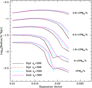
The physical radius of a sphere containing a fixed amount of mass in a simulation of the formation of a massive halo at high redshift. The sphere is centred on a density maximum located by applying the shrinking sphere algorithm detailed in the text. The four curves show simulations starting from either Zel'dovich or 2lpt initial conditions, at a start redshift of 399 or 599. The agreement between the two 2lpt initial conditions is very good. As expected from the spherical collapse model, discussed in Section 2.2, the collapse of the Zel'dovich initial conditions is delayed with the largest delay occurring for z_s= 399.

Open in new tabDownload slide

The collapse occurring in the R5 simulation is only approximately spherical as evidenced by figs 3 and 4 in Gao et al. (2005). It is nonetheless interesting to see whether the results from the spherical top-hat model do agree quantitatively as well as qualitatively. To do this, we first estimated an expansion factor of collapse for each of the five 2lpt z_s= 599 curves, by fitting a spherical top-hat to each curve and taking a value for the expansion factor of collapse from the corresponding top-hat model. We chose these particular curves because the expected timing error for these 2lpt initial conditions should be very small, compared to the simulations started from Zel'dovich initial conditions, and so should not bias the estimate of the collapse expansion factor significantly. In Fig. 4, the same radii are plotted as in Fig. 3. However, the values of the expansion factors along the x-axis are ‘corrected’ using the equations (13) and (14) to cancel out the expected timing errors for both the 2lpt and Zel'dovich initial conditions. The timing error is assumed constant along each curve. Strictly speaking, this correction applies at the moment the spherical top-hat solution collapses to a point. However, inspection of Fig. 1, together with the fact that top-hat solution is symmetric in time, for any initial condition, about the point of maximum expansion (for an Einstein-de Sitter universe, an excellent approximation at redshift ∼50), shows that the timing error mostly arises around the time of maximum expansion and therefore the correction at the time of collapse should be applicable once the top-hat has collapsed by more than ∼0.85 of the radius of maximum expansion. For the spherical top-hat, this corresponds to the density exceeding the critical density by a factor of about 10, and this overdensity is marked on each curve in Fig. 4 by a black dot. To the left of the dots, the density is less than 10 so the correction is expected to be too strong, which it is. To the right of the dots, the shift works rather well with the lines showing much better agreement than in Fig. 3. The spacing of the outputs is too crude to follow the collapse of the innermost two radii very accurately, so it is not surprising the agreement around a= 0.018 is less good than elsewhere.

Figure 4

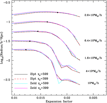
Same as Fig. 3 except that the expansion factor plotted for each of the four curves has been corrected to account for the time delay expected in the spherical collapse model and given by equations (13) and (14). The density inside each radius exceeds 10 times the critical density to the right of the black dots. The correction is expected to work well for a spherical collapse above an overdensity of around 10 (see the main text). Even though the collapse is not perfectly spherical applying the correction does greatly improve the match between the four curves particularly to the right of the black dots. The spacing of the outputs is insufficient to resolve features around a= 0.018 where shell crossing becomes important in the lower two curves.

Open in new tabDownload slide

In conclusion, the results using 2lpt initial conditions are much less sensitive to the start redshift and it is possible to start the simulation later. The formation of the halo is delayed using Zel'dovich initial conditions and the magnitude the delay agrees with what one would expect for a spherical top-hat collapse.

4.2 Aquarius haloes from 2lpt initial conditions

As a final example, we look at the effect of using 2lpt resimulation initial conditions on the redshift zero internal structure of one of the Aquarius haloes (Springel et al. 2008). The start redshift of the Aquarius haloes was 127, so even for a spherical top-hat collapse the timing error given by equation (11) would only be around 90 Myr for Zel'dovich initial conditions, which is short compared to the age of the Universe, so any effects on the main halo are expected to be small.

We chose the Aq-A-5 halo, with about 600 000 particles within r₂₀₀, from Springel et al. (2008) as a convenient halo to study the effects of varying the start redshift and initial conditions. For this study, we ran eight (re)simulations of Aq-A-5 to redshift zero, starting at redshifts 127, 63, 31 and 15, for both Zel'dovich and 2lpt initial conditions. We used the p-gadget3 (which is needed to create the 2lpt initial conditions) and took identical values for the various numerical parameters as in Springel et al. (2008), and similarly ran the subfind algorithm to identify subhaloes. At this resolution, there are typically about 230 substructures with more than 31 particles in the main halo.

In Fig. 5, we show the circular velocity as a function of radius for Aq-A-5 halo at redshift zero for all eight simulations. The radius is taken from the position of the potential minimum identified by subfind (Springel et al. 2001), and the circular velocity is computed assuming spherical symmetry for the mass distribution about the potential minimum. Comparing the circular velocities for the Zel'dovich initial conditions amongst themselves, and likewise the 2lpt circular velocities (displaced vertically by 30 km s⁻¹ for clarity) it is first evident that the circular velocity curves are almost all rather alike, with the simulation starting from z_s= 15 Zel'dovich initial conditions being the outlier. For these initial conditions, the peak of the circular velocity at z= 0 occurs almost 50 per cent further from the centre than in the other simulations. Comparing the curves, it is clear that the circular velocity shows a much weaker dependence on the start redshift with the 2lpt initial conditions than with Zel'dovich initial conditions.

Figure 5

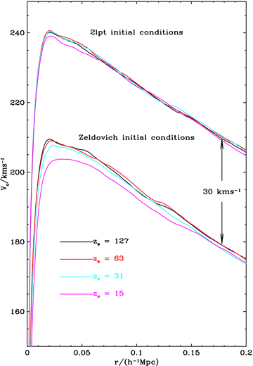
The circular velocity as a function of radius for the Aquarius Aq-A-5 halo at z= 0 for simulations starting from 2lpt initial conditions (shifted vertically by 30 km s⁻¹ for clarity) and Zel'dovich initial conditions, starting from the redshifts indicated in the key. The curves for 2lpt initial conditions are much more consistent amongst themselves. The Aquarius Aq-A-5 halo in Springel et al. (2008) was started at z_s= 127 from Zel'dovich initial conditions. In the absence of the 30 km s⁻¹ vertical shift, the z_s= 127 curve starting from Zel'dovich initial conditions lies between or very close to the 2lpt circular velocity curves.

Open in new tabDownload slide

In Fig. 6, we plot the cumulative subhalo abundance as a function of the maximum subhalo circular velocity for the eight simulations, shifting the Zel'dovich curves upward by 1 dex for clarity. Again, the subhalo circular velocity functions show a much greater consistency at z= 0 amongst the simulations starting from 2lpt initial conditions compared with Zel'dovich initial conditions.

Figure 6

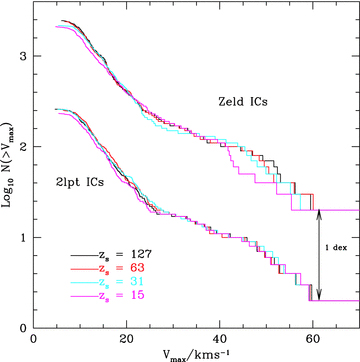
Cumulative subhalo abundance as a function of the maximum subhalo circular velocity for Aquarius halo Aq-A-5 run starting at redshift, z_s, with Zel'dovich and 2lpt resimulation initial conditions. The results from the 2lpt initial conditions are less sensitive to the start redshift. The cumulative function for the Zel'dovich initial conditions have been shifted upwards by 1 dex for clarity. The curve obtained by plotting the Zel'dovich z_s= 127 with the shift lies within or close to the curves from the 2lpt initial conditions.

Open in new tabDownload slide

Finally, in this section we look at the sensitivity of the position of subhaloes inside the Aq-A-5 halo, as determined by subfind, to the start redshift and kind of initial conditions. A comparison of the relative subhalo positions for the Aq-A halo resimulated at different resolutions was presented in Springel et al. (2008). For these simulations, it proved possible to identify corresponding substructures in the different simulations and compare their relative positions. All of these simulations were started from the same start redshift with Zel'dovich initial conditions so the details of the comparison are not directly relevant, nonetheless the fact that differences of similar magnitude to those found here occur implies that there are other numerical issues which also affect the positions of substructures significantly.

We can likewise match substructures between our simulations, and this is made easier by the fact that there is a one-to-one correspondence between the dark matter particles in the different resimulations based on their Lagrangian coordinates. To make the a fair comparison between all 28 pairs of simulations, we first found a subset of matched subhaloes common to all eight resimulations. This sample has only 50 members. This compares to between 102 and 180 matches between the different pairs of simulations. The failure to match can arise from two boundary effects: a subhalo in one simulation may be a free halo in the other and a ‘subhalo’ may be below the limit of 32 particles in one of the simulations. Almost half of the subhaloes found have less than 64 particles.

The subhalo positions in two different simulations are compared, after first subtracting the position of the main subhalo. There are many ways to compare the differences found. We have selected to show the geometric mean of the distance between matched subhaloes between pairs of simulations in Fig. 7. Comparisons based on other quantities such as the mean or median separation give qualitatively similar results.

Figure 7

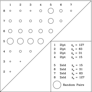
Sensitivity of the subhalo positions to the start redshift and type of initial condition. Each circle above the diagonal represents the result of a comparison, made at z= 0, between two resimulations out of a total of eight resimulations of halo Aq-A-5. The type of initial condition and the start redshift, z_s, are given in the figure legend. The radius of each circle is equal to the geometric mean distance between a sample of matched subhaloes, common to all eight resimulations. For scale, the circle in the legend has a radius of 192 kpc h⁻¹ which corresponds to the geometric mean separation, averaged over all eight resimulations, between randomly chosen pairs of subhaloes within the same halo. The 2lpt initial conditions are significantly less sensitive to the start redshift than Zel'dovich initial conditions.

Open in new tabDownload slide

Again we find, from Fig. 7, that the simulations started from 2lpt initial conditions show much less variation in position on the start redshift than Zel'dovich initial conditions. For the simulation with Zel'dovich initial conditions starting from z_s= 15, the location of the subhaloes is very poorly correlated with any other of the simulations, although still better than the geometric mean separation of all non-identical pairs of subhaloes in any given halo. Starting the Zel'dovich initial conditions at z_s= 127, the starting redshift for the Aquarius haloes does give subhalo positions which match the 2lpt resimulation subhalo positions fairly well. We checked that the analogous plot produced using the larger matched subhaloes between each pair, rather than the subsample of subhaloes common to all eight simulations, gives a very similar plot to the plot shown.

In conclusion, for a resimulation of a Milky Way like dark matter halo it is clear that the z= 0 properties of the halo do depend somewhat on the start redshift, but that dependence is much reduced with 2lpt resimulation initial conditions. The evolution of the halo to z= 0 is highly non-linear, but the results are qualitatively in agreement with the known behaviour of 2lpt and Zel'dovich initial conditions in the quasi-linear regime (Scoccimarro 1998) where this can be understood from the behaviour of transients which are both smaller and decay faster (by a factor of 1 +z) for 2lpt initial conditions than for Zel'dovich initial conditions. In quantitative terms, the differences amongst the circular velocity curves, the cumulative subhalo abundances and the relative positions of substructures between the different simulations started from 2lpt initial conditions, are larger than naively expect from the behaviour of transients. This is most likely because there are other numerical factors which lead to much of the differences seen in the various simulations starting from 2lpt initial conditions.

To show this is indeed the case, we repeated one resimulation using initial conditions that were mirror reflected about the centre of the periodic volume. Running these otherwise identical simulations leads, after reflecting the final conditions, to differences in the positions of the subhaloes. The numerical process of mirroring is not a perfect symmetry operation when operated on double precision floating point numbers so in effect the comparison shows that the effects of rounding error in the positions can propagate to much larger scales. After matching 189 subhaloes for the z= 0 haloes, we find the geometric separation of the subhaloes between these reflected initial conditions is 12 kpc h⁻¹. This can be compared to 26 kpc h⁻¹ difference between the 175 matched subhaloes between the 2lpt resimulations starting at redshifts 127 and 63. This kind of sensitivity to the initial conditions is expected given that halo formation is a strongly non-linear processes. It is interesting however, even though these simulations of halo formation show this kind of sensitivity to small changes in the initial conditions, that the effects of starting from 2lpt or Zel'dovich initial conditions are still apparent at redshift zero for many properties including for the circular velocity curve, the subhalo velocity functions and subhalo positions.

5 SUMMARY AND DISCUSSION

We have implemented a new method to make 2lpt initial conditions which is well suited to creating resimulation initial conditions. We have tested the method for an analytic spherically symmetric perturbation with features ranging over a factor of 5000 in linear scale or 11 orders of magnitude in mass, and can reproduce the analytic solution to a fractional accuracy of better than one per cent over this range of scales in radius measured from the symmetry centre.

Applying the new method, we have recreated the initial conditions for the formation of a high-redshift halo from Gao et al. (2005) and the a Milky Way mass halo from Springel et al. (2008). We find from studying the properties of the final haloes that the final conditions show much less sensitivity to the start redshift when using 2lpt initial conditions than when started from Zel'dovich initial conditions.

For didactic purposes, we have calculated the effect of using Zel'dovich and 2lpt initial conditions for a spherical top-hat collapse. In this simple case, the epoch of collapse is delayed by a timing error which depends primarily on the number of expansions between the epoch of the initial conditions and the collapse time. This timing error, for fixed starting redshift, grows with collapse time for Zel'dovich initial conditions, but decreases with collapse time for 2lpt initial conditions. Applying the top-hat timing errors as a correction to the radius of shells containing fixed amounts of mass as a function of time has the effect of bringing the Zel'dovich and 2lpt resimulations of the high-redshift Gao et al. (2005) halo into near coincidence.

We find that for the Aq-A-5 halo the choice of start redshift for the Zel'dovich initial conditions in Springel et al. (2008) was sufficiently high at z_s= 127 to make little difference to the properties of the halo at z= 0 when compared to runs starting from 2lpt initial conditions. For lower starting redshifts (z_s= 63, 31, 15), the positions of substructures at z= 0 do become sensitive to the precise start redshift.

Knebe et al. (2009) have also looked at the properties of haloes, for the mass range (10¹⁰−10¹³h⁻¹M_⊙) at redshift zero, for simulations starting from Zel'dovich and 2lpt initial conditions (generated using the code by Crocce et al. 2006). In their paper, they simulated a cosmological volume which yielded many small haloes and about 10 haloes with 150 000 or more particles within the virial radius. In their study, they looked at the distribution of halo properties including the spin, triaxiality and concentration. They also matched haloes in a similar way to the way we have matched subhaloes and looked at the ratios of masses, triaxialities, spins and concentrations of the matching haloes. The authors concluded that any actual trends with start redshift or type of initial condition by redshift zero are certainly small (for start redshifts of 25–150). It is not possible to directly compare our results with theirs, but the trends in the halo properties we have observed in halo Aq-A-5 at redshift zero are indeed small, and not obviously in disagreement with their results for populations of haloes.

For many purposes, the differences which arise from using Zel'dovich or 2lpt initial conditions may be small when compared to the uncertainties which arise in the modelling of more complex physical processes. From this point of view, the main advantage of using 2lpt initial conditions is that they allow the simulations to start later thus saving computer time. The issue of exactly what redshift one can start depends on the scientific problem, but the spherical collapse model discussed in Section 2.2 gives a quantitative way to compare the start redshift for Zel'dovich or 2lpt initial conditions. However, it remains the case that it is advisable to test the sensitivity of simulation results to the start redshift by direct simulation as for example in Power et al. (2003) for resimulations of galactic dark matter haloes.

I would particularly like to thank Volker Springel for implementing part of the method described in this paper in his p-gadget3 code and for reading a draft of this paper. I would also like to thank Roman Scoccimarro for clarifying an issue connected with the second-order overdensity field early on in this project, Gao Liang, for helping with remaking the Gao et al. (2005) initial conditions and Carlos Frenk for comments on the first draft. The simulations in this paper were run on COSMA and I am grateful to Lydia Heck for computer support. This work was supported by STFC rolling grant ST/F002289/1.

REFERENCES

Appendix

APPENDIX A: METHODS FOR INTERPOLATION OF DISPLACEMENT FIELDS

As mentioned in the main text, it is necessary to use interpolation of the displacement fields when making resimulation initial conditions in order to find the displacements at the particle positions. This need arises for example because the interparticle spacing in the high-resolution region of the resimulation initial conditions is typically many times smaller than the Fourier grid used to generate the longest wavelength displacements over the entire periodic simulation volume. Another situation where interpolation is needed, even for cosmological initial conditions, occurs when the particle load is based on a glass-like distribution (White 1996) which means the particles cannot coincide with the grid points.

In this appendix, we will examine two interpolation methods which are in use and compare them. We will simplify the discussion to the case in the limit of the interparticle separation going to zero creating a continuous and uniform density medium. We assume that the displacement field is built of a finite number of plane waves and that the displacements are known precisely on a regular cubic grid of points. The purpose of the interpolation is to reconstruct the displacement field everywhere between these grid points. The success of a particular interpolation scheme can be judged by comparing the density field created by applying the displacements given by interpolated displacement field with the density field generated from the true displacement field. We will assume the displacements are small so there is no shell crossing and further consider only the linear dependence of the density field on the displacements. The interpolation schemes we consider use linear combinations of the values known at the grid points, so it is sufficient to characterize the interpolation scheme by applying it to plane waves.

We will compare the performance of two interpolation schemes: the first, trilinear interpolation (TLI) or Cloud-in-Cell, Hockney & Eastwood (1988), has been used for making initial conditions over many years for example in the Hubble Volume Simulations (Evrard et al. 2002) and the Millennium Simulation (Springel et al. 2005) as well as resimulation initial conditions (e.g. Gao et al. 2005). The second method, not previously documented, which we call QI, for quadratic interpolation, has been used more recently for the Aquarius initial conditions (Springel et al. 2008).

In principle, because the displacement fields for resimulations are generated by Fourier methods are bandwidth limited, the interpolation of the displacement field to the particle positions can be done perfectly using the Whittaker–Shannon interpolation formula (Press et al. 1992). This is impractical because the sum must be taken over all grid points. The only exception to this is the trivial case where the particles lie on the Fourier grid points themselves, in which case no interpolation is needed. For cosmological initial conditions, unlike resimulation initial conditions, this can easily be arranged, as for example in the 2lpt initial condition code made available by Crocce et al. (2006).

Before discussing particular interpolation formulae, we first define some convenient notation. Suppose the computational domain is a periodic cube of side length L and that we define a cubic grid with p³ cubic cells of side length Δ such that L=pΔ. A general point in the volume has coordinates (x, y, z) where all three spatial coordinates have a range 0 ≤x, y, z < L. We will consider the interpolation of a scalar field A(x, y, z) and assume A a bandwidth-limited function, in such a way that its value can be predicted exactly anywhere within the domain using the Whittaker–Shannon interpolation formula and summing over the p³ grid points.

We first consider TLI. The interpolated field, A_TLI, is given by the expression:

(A1)

where the (l₁, l₂, l₃) represents an integer triplet and the sum is over all p³ grid points. For TLI, the kernel W is defined as

(A2)

TLI is exact for a function which is a sum of terms where 0 ≤α_i≤ 1. The compact form of W means that to evaluate the interpolated field at the position of a particle it requires summing only eight terms corresponding to the nearest grid points. The resulting field, A_TLI, is continuous everywhere, which is a necessary requirement when interpolating a component of the displacement field, otherwise regions of zero or double density can be created along the interfaces marking the discontinuities. When TLI is applied to the components of the displacement field, the resulting density field has discontinuities.

We will now consider the effect on a plane wave. The ‘interpolated’ wave will no longer be a simple plane wave but a superposition of the ‘fundamental’ plane wave (with a reduced amplitude) and the harmonics of the fundamental wave. The same is true of the density field generated by applying the interpolated displacements (assumed normal to the plane wave and of small amplitude) to a uniform medium. The relative power in the fundamental wave and the harmonics will differ between the displacement field and the density field, with relatively more power in the density field harmonics. The ideal interpolation scheme minimizes the power in these harmonics and maximizes the power in the fundamental plane wave.

Consider a plane wave mode in a periodic cube of side-length L:

(A3)

where k₁, k₂, k₃ are integers and B is the amplitude of the wave. It is straightforward to show that applying TLI to the plane wave gives a reduced amplitude, B_TLI, for the fundamental plain wave given by the following ratio:

(A4)

where u_i=πk_i/p provided 0 < u_i≤π/2.

This factor applies equally to the displacement field and the linear density field created by applying the interpolated displacement field to a uniform medium. For small values of u_i, the ratio is close unity and deviates below unity quadratically to lowest order. It is desirable to use as large a Fourier grid as memory allows for making resimulation initial conditions to minimize the interpolation error.

The interpolation can be made more accurate if the derivatives of the field, A, are also known at the grid points. The derivatives of the displacement field need to be computed for 2lpt initial conditions in any case and it was the fact that the derivatives need to be calculated anyway that motivated trying to find an improved interpolation scheme making use of them.

It is straightforward, making use of the derivatives of the field to devise a formula which is exact for linear and quadratic functions of the coordinates. We will call it the quadratic scheme. The field A_QI is given by

(A5)

where

(A6)

QI is exact for any function which is a sum of terms where 0 ≤α_i≤ 2. The three additional terms in the QI formula vanish at the grid points so like TLI formula the QI scheme is exact at the grid points. The corresponding effect of QI on a plane wave can be shown to be

(A7)

where u_i=πk_i/p provided 0 < u_i≤π/2. Again, this ratio is close to unity, when u_i is small, but the leading order deviation below unity for small u_i is now quartic – a considerable improvement.

Fig. A1 compares the two interpolation schemes acting on a plane wave along one of the principal coordinate axes. The upper curves show the ratio of the power in the density field created by applying the interpolated displacements with the true power for both the TLI and QI schemes. The curves are obtained by setting u₂= 0; u₃= 0 in equations (A4) and (A7), respectively, and the x-axis is plotted up to the Nyquist wavenumber of the Fourier grid points where the displacement field is known exactly. Both the interpolation schemes introduce power into the harmonics of the plane wave. For a one-dimensional plane wave, the TLI scheme this harmonic power can be shown to be

(A8)

while for the QI scheme the harmonic power is given by

(A9)

where u=kπ/p provided 0 < u≤π/2. The lower two curves show the amount of power generated in the harmonics for the TLI and QI schemes. The QI scheme is evidently superior to TLI on both measures.

Figure A1

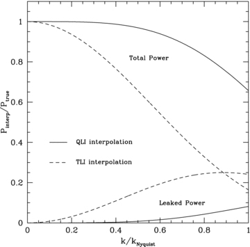
The curves show the effects of the TLI and QI schemes when applied to a one-dimensional plane wave, representing a displacement field normal to the wave, of wavenumber k, given a sampling rate of the plane wave of wavenumber k_Nyquist. The upper curves show the power remaining in resulting linear density created by displacing a uniform medium, with the plane wave displacements given by interpolation, while the lower curves show the power introduced into the harmonics of the plane wave by the process of interpolation.

Open in new tabDownload slide

Both the TLI and QI schemes have cubic symmetry, and therefore generate some anisotropies. However, in both schemes these anisotropies are small and enter first at quartic order in the magnitude of the wavevector. The fractional rms derivation in the power in the fundamental wave about the average over all directions less than 1 per cent even at the Nyquist wavelength for both the TLI and QI, with QI being the best by a factor of 3.

For a fixed grid size, implementing the QI formula is a factor of 4 more expensive than TLI as the three derivatives of A need to be computed in addition to A itself. For initial conditions, this factor is reduced to 3, because the quantities of interest are gradients of a potential which reduces the number of independent terms that have to be evaluated. The QI scheme, however, is more attractive after taking account of its improved accuracy and the fact that the computational effort scales approximately as the cube of the dimension of the Fourier grid. For limited memory or limited CPU, the QI scheme is to be preferred to TLI.

The QI scheme was used for making all the Zel'dovich and 2lpt initial conditions used in this paper. For the derivatives of the Zel'dovich displacements, which are required to compute the second-order overdensity, using the QI scheme entails calculating the second-order derivatives of the Zel'dovich displacements.