Alternative diagnostic diagrams and the ‘forgotten’ population of weak line galaxies in the SDSS Free

Abstract

1 INTRODUCTION

Galaxies with emission lines can reveal more of their secrets than those without. The strength and pattern of emission lines convey information on the power and nature of the ionizing source, the geometry, physical conditions and chemical composition of the gas, as well as on the dust content of emitting regions. Even when these properties cannot be determined unambiguously, emission-line data allow one to assign galaxies to physically motivated classes, such as star forming (SF) or hosts of active galactic nuclei (AGN), and to split them into finer categories such as high-ionization (Seyfert) and low-ionization nuclear emission-line region (LINER) sub-types.

The classification of emission-line galaxies (ELGs) is usually done through emission-line ratio diagnostic diagrams. Baldwin, Phillips & Terlevich (1981) were the first to propose such a scheme. Their [O iii]/Hβ versus [N ii]/Hα diagram1 (the ‘BPT diagram’), in particular, became the benchmark for emission-line classification. In their original plot, H ii regions, planetary nebulae, Seyfert nuclei and LINERs occupied well-isolated regions, demonstrating the diagnostic power of this combination or flux ratios. As data accumulated through the 1980s and 1990s (Veilleux & Osterbrock 1987; Ho, Filippenko & Sargent 1997; Véron-Cetty & Véron 2000), a more continuous distribution gradually emerged, culminating with the Sloan Digital Sky Survey (SDSS; York et al. 2000), which allowed the mapping of the BPT plane with over 10⁵ data points (Kauffmann et al. 2003, hereafter K03), revealing the now familiar seagull-like shape, with two well-defined wings.

The left wing arises due to a strong coupling between the O/H and N/O abundance ratios, the ionizing radiation field and the ionization parameter in SF galaxies (McCall, Rybski & Shields 1985; Dopita & Evans 1986). Empirical and model-based frontiers have been drawn in the [O iii]/Hβ–[N ii]/Hα space to delineate the SF territory from the rest (Kewley et al. 2001, hereafter K01; K03; Stasińska et al. 2006, hereafter S06). Galaxies above these dividing lines have their collisionally excited lines ([O iii], [N ii] etc.) stronger with respect to recombination lines (Hα, Hβ) than SF galaxies, signalling photoionization by a radiation field harder than that produced by massive young stars.

The right wing is populated by galaxies with Seyfert-like or LINER-like spectra.2 Recently, taking advantage of the huge number of galaxy spectra available in the SDSS, Kewley et al. (2006, hereafter K06) identified a split of the right wing into Seyfert and LINER branches, better seen in the [O iii]/Hβ–[S ii]/Hα and [O iii]/Hβ–[O i]/Hα diagrams, but also visible in the BPT. The physics behind this dichotomy, and indeed of right-wing sources as a whole, is far less understood than that behind the SF wing. Moreover, as argued by Stasińska et al. (2008) observational selection effects play a key role in shaping the right wing, and both stellar and non-stellar ionizing sources can be present.

Notwithstanding these interpretational caveats, for both physical and practical reasons the BPT diagram has been the main workhorse for emission-line classification for nearly three decades. The basic requirement for a reliable BPT classification is that Hβ, [O iii], Hα and [N ii] are all detected above some minimum signal-to-noise ratio (SN_λ). SDSS papers usually adopt a uniform SN_λ≥ 3 cut (K03; Brinchmann et al. 2004; Li et al. 2006). This quality control charges a large toll in terms of the number of excluded objects. The scale of this problem is often overlooked (see, however, Miller et al. 2003; Best et al. 2005; Hao et al. 2005). As shown here, for the SDSS as a whole, about one in three ELGs has Hβ and/or [O iii] below this threshold. More worryingly, the overwhelming majority of these excluded galaxies belong to the right wing, where about two in every three sources suffer from line weakness.

Clearly, no quantitative nor qualitative picture of ELGs in the local Universe can be complete ignoring weak line galaxies (WLGs). This is the basic motivation behind this work, whose main goal is to rescue this numerous, yet often forgotten population of galaxies from the classification limbo. The physical nature of WLGs will be discussed in a forthcoming communication.

This paper is structured as follows. After presenting the sample and basic data-processing steps (Section 2), we assess the size of the WLG population in the SDSS and define sub-types of WLGs based on which lines prevent a reliable spectral classification (Section 3). In Section 4, we propose alternative diagnostics diagrams which help in placing WLGs in the standard framework of emission-line categories. Section 5 presents an objective method to transpose the most popular SF/AGN and Seyfert/LINER dividing lines to our more economic diagnostic diagrams. These new and more inclusive diagrams allow the classification of WLGs, leading to a revised census of ELGs in the nearby Universe, presented in Section 6, which also discusses how WLGs affect the Seyfert/LINER dichotomy. Section 7 summarizes our conclusions. Hurried readers in search of spectral classification criteria may want to jump straight to Section 5.6, where equations to separate SF from AGN and Seyferts from LINERs are presented.

2 DATA

2.1 Sample selection

The data used in this study come from the seventh data release (DR7) of the SDSS (Abazajian et al. 2009). We start from a raw sample of 926 246 galaxies analysed with the starlight code (Cid Fernandes et al. 2005) and apply an initial cut to objects within the SDSS Main Galaxy Sample (Strauss et al. 2002). This leaves nearly 700 000 galaxies and already excludes objects with broad emission lines. A final sample of ∼370 000 galaxies is culled from this list by applying the following criteria.

Since we are interested in objects with weak emission lines, we removed all spectra where artefacts such as bad pixels, imperfect sky-subtraction or lack of data prevent a clean measurement of any of the following lines: [O ii], Hβ, [O iii], Hα and [N ii]. In practice, we require no faulty pixel within ±15 Å of these lines. This guarantees when any one of these lines is not detected it is because it is really immersed in the noise or altogether absent, instead of due to some technical problem. This conservative cut alone imposes a substantial (42 per cent) reduction on the sample. Few galaxies outside the 0.024–0.17 redshift interval survive this ‘clean lines only’ cut, so, to round up numbers, we further exclude galaxies outside this range. We further trimmed the sample by requiring a lower limit of 10 for the signal-to-noise ratio in the 4730–4780 Å continuum. This is done to ensure that enough signal is present to allow a meaningful stellar population fit, necessary for the measurement of emission lines, particularly weak ones.

These criteria lead to a sample of 371 084 galaxies, hereafter our ‘main sample’. The restriction to good fluxes around the wavelengths of the main emission lines introduces some peculiarities, such as z gaps when [O iii] and Hβ move into the region around the 5577 Å sky line. Since all demographic arguments will be restricted to within the sample, such peculiarities do not pose a problem.

None of our selection criteria favours the inclusion of emission-line systems, yet the overwhelming majority of galaxies in our sample do present emission lines. For instance, 82 per cent of them have at least one of Hα or [N ii] with SN_λ≥ 3. This highlights the fact that emission lines are nearly ubiquitous and the importance of understanding their origin.

2.2 starlight processing and emission-line measurements

Spectra for all galaxies were processed with version 05 of the spectral synthesis code starlight, which performs pixel-by-pixel fits of the stellar continuum, delivering a long list of physical properties as well as pure emission spectra from which emission-line measurements are performed (Cid Fernandes et al. 2005). The code itself and its results for the entire SDSS-DR5 data base are available in a Virtual Observatory (VO)-like environment at http://www.starlight.ufsc.br, and products for the whole DR7 will become available shortly.

As in previous papers in this series, the spectral fits are based on the Bruzual & Charlot (2003) models with the STELIB library (Le Borgne et al. 2003), ‘Padova 1994’ tracks (Bertelli et al. 1994) and Chabrier (2003) initial mass function. These models are being superseded by a new vintage of evolutionary synthesis calculations incorporating improvements in the stellar tracks and spectral libraries, which should affect galaxian properties derived from spectral synthesis codes such as starlight. These new models also provide measurably better spectral fits, leading to differences in emission-line measurements. The differences are not large, but may be significant for intrinsically weak lines. A full assessment of these effects will have to await the release of these new models, but experiments based on preliminary versions indicate that the main results of this study remain valid (Gomes 2009).

A difference with respect to the latest papers of the SEAGal collaboration (Asari et al. 2007; Cid Fernandes et al. 2007; Stasińska et al. 2008; Vale Asari et al. 2009), which used DR5 data, is that we are now working with DR7. In addition to the increase by ∼60 per cent in the number of galaxies with respect to DR5, there have been changes in the reduction pipeline which propagate to differences in the amplitude and shape of the spectra (Adelman-McCarthy et al. 2008; Abazajian et al. 2009).

Emission lines are measured fitting Gaussians to the residual spectrum obtained after subtraction of the starlight fit. The Gaussians can have different widths and offsets, with constraints imposed on lines from similar ionization levels. Details on this procedure are given in S06.

As noted by Asari et al. (2007), the Bruzual & Charlot (2003) models have a low amplitude hump in the ∼100 Å interval around Hβ, such that Hβ emission often sits in a slightly negative valley in the observed minus model spectrum (an artefact of the STELIB library, which disappears when using models based on the MILES library of Sánchez-Blázquez et al. 2006). Asari et al. (2007) found this effect to be unimportant for their Hβ measurements, but their analysis focused on SF galaxies, which tend to have strong Hβ. Here it has a larger impact, since we are specifically interested in galaxies with intrinsically weak Hβ. To alleviate this problem, the Hβ flux measurements were performed with respect to a local ‘continuum’ in the residual spectrum. No such systematic residual is found for other emission lines, whose measurement does not require the extra care devoted to Hβ.

3 THE POPULATION OF GALAXIES ELIMINATED BY LINE QUALITY CUTS

Throughout this paper, a galaxy is said to be an ELG if both Hα and [N ii] are detected with a signal-to-noise ratio of 3 or better. Out of the 371 084 galaxies in our main sample, 280 495 (76 per cent) match this definition. Many of these, however, have Hβ and [O iii] data which would be considered unusable by most standards. This section quantifies this population and introduces the WLG notation used in later sections.

3.1 The dramatic effect of SN_λ selection

A first assessment of the dimension of the WLG population can be obtained from the distributions of SN_λ for the main optical emission lines. Brinchmann et al. (2004) have carried out such an analysis for their DR1 data; in particular, their fig. 2 shows histograms of SN_λ for the main lines. Our results are shown in Fig. 1, where we plot the cumulative SN_λ distribution for [O ii] and the four BPT lines.

Figure 1

Cumulative distributions of the signal-to-noise ratio for [O ii], Hβ, [O iii], Hα and [N ii] for our main sample (see Section 2.1). (a) All galaxies. (b) Only those with (right-wing sources in the BPT diagram). (c) Only galaxies above the K01 ‘extreme starburst’ line in the BPT plane, often dubbed ‘pure AGN’ (but see Section 5.1). In all panels a filled circle marks the number of galaxies with SN_Hα and SN_{[N ii]}≥ 3 (our definition of ELG), while the empty circle corresponds to SN_λ≥ 3 in all four BPT lines (called ‘SLGs’ in this paper), and a triangle marks the number of galaxies with Hβ, [O iii], Hα, [N ii] plus [O i] and the [S ii] lines detected at SN_λ≥ 3. Note the huge effect of imposing a SN_λ≥ 3 cut on lines other than Hα and [N ii], particularly for non-SF galaxies (panels b and c).

Open in new tabDownload slide

The left-hand panel shows that Hβ and [O iii] are the weakest of the BPT lines for the main sample as a whole. Of the 280 495 galaxies which satisfy our definition of ELG, i.e. SN_Hα and SN_{[N ii]}≥ 3 (marked with a filled circle in the plot), only 188 052 also have SN_Hβ and SN_{[O iii]}≥ 3, as indicated by the open circle. The responsibility for this 33 per cent global reduction is approximately equally shared between Hβ and [O iii].

It is crucial to realize that galaxies excluded by a uniform SN_λ cut are not just a random population which would spread evenly among strong line sources in the BPT diagram had their spectra been collected with better signal. To illustrate this, Fig. 1(b) shows the SN_λ cumulative distributions for the subset of galaxies with ⁠, a criterion which completely excludes left-wing sources (S06). The Hβ curve is now well below the one for [O iii] for any value of SN_λ. Of the 105 414 ELGs in this plot, 74 per cent also have SN_{[O iii]}≥ 3, but only 47 per cent have SN_Hβ≥ 3. Requiring both Hβ and [O iii] to have SN_λ≥ 3 reduces the sample to 41 per cent (open circle). Clearly, weak or undetected Hβ emission is the main culprit for this dramatic (factor of 2.4) drop in numbers of galaxies in the right wing. A caveat with this plot is that the [N ii]/H α ratio, used to select right-wing sources, is computed for all galaxies where both lines are ‘detected’, i.e. SN_λ≥ 1. For the lowest SN_λ values, this ratio is highly uncertain, but since over 83 per cent of the sources in Fig. 1(b) have SN_{[N ii]} and SN_Hα≥ 3, contamination by non-right-wing sources is small.

Fig. 1(c) repeats this numerology including only objects above the K01 ‘extreme starburst’ line in the BPT plane, leaving only sources normally interpreted as ‘pure AGN’, i.e. AGN whose lines are little or not contaminated by SF (but see Section 5.1 for a criticism of this reading). In this case, just 43 per cent of the objects have SN_λ≥ 3 in all four lines involved in the selection process, and thus the results should be taken as indicative only. Caveats aside, the general message conveyed by this plot is the same as that spelt by Fig. 1(b), namely that low SN_λ emission lines occur more frequently among AGN-like galaxies.

Finally, in all panels of Fig. 1 a triangle marks the result of requiring 3σ or better detections of all BPT line plus the [O i] and [S ii] lines, all of which are explicitly used in the K06 Seyfert/LINER classification scheme. Clearly, the implied exclusion factors are prohibitively large.

To summarize:

• WLGs comprise a large (∼1 in 3) fraction of ELGs in the SDSS;

• line weakness is much more severe in the right wing of the BPT diagram, where nearly half of the sources fail an SN_λ≥ 3 cut for all the BPT lines;

• further requiring good [O i] and [S ii] measurements implies approximately two times larger exclusion factors.

3.2 Weak line galaxies of different kinds: definitions

We define a WLG as a galaxy whose Hα and [N ii] lines are both detected with SN_λ≥ 3, but either or both of Hβ and [O iii] have lower SN_λ. In other words, a WLG is an ELG with weak Hβ and/or weak [O iii]. Conversely, galaxies where all four BPT lines have SN_λ≥ 3 will be called ‘strong line galaxies’ (SLGs). WLGs and SLGs comprise 33 and 67 per cent of our ELG sample, respectively (but recall from fig. 1 that these proportions are approximately inverted in the right wing).

With this definition, WLGs fall into one of three possible kinds:

• WL-H: weak Hβ(SN_Hβ < 3) but strong [O iii](SN_{[O iii]}≥ 3);

• WL-O: weak [O iii](SN_{[O iii]} < 3) but strong Hβ(SN_Hβ≥ 3);

• WL-HO: weak Hβ(SN_Hβ < 3) and [O iii](SN_{[O iii]} < 3).

The WL-H, WL-O and WL-HO denominations are introduced merely to identify which emission lines are too weak (or missing) to allow a solid spectral classification. These are not meant to be interpreted as new spectral classes. On the contrary, our goal here is precisely to find out where these objects fit into the current emission-line taxonomical paradigm.

The populations of WLGs of types WL-H, WL-HO and WL-O are comparable in size: N_WL-H= 38 631, N_WL-HO= 25 805 and N_WL-O= 28 007. Note that WLGs include objects where Hβ and/or [O iii] are not detected at all (SN_λ < 1). Such non-detections are genuinely due to line weakness, since we have excluded sources with faulty pixels around emission lines (see Section 2.1). [O iii] is undetected in 15 per cent (4288) of WL-Os, while Hβ is undetected in 25 per cent (9531) of WL-Hs. Among WL-HOs, 8059 (31 per cent) have no Hβ, 5773 (22 per cent) have no [O iii] and 1965 (8 per cent) have neither. Excluding non-detections, WL-Hs have median SN_λ values of 1.9 in Hβ, 4.5 in [O iii], 7.4 in Hα and 7.6 in [N ii]. For WL-HOs, SN_Hβ= 1.7, SN_{[O iii]}= 2.1, SN_Hα= 6.0 and SN_{[N ii]}= 5.7, while for WL-Os, SN_Hβ= 6.0, SN_{[O iii]}= 2.3, SN_Hα= 24.8 and SN_{[N ii]}= 13.4.

We point out that our definition of ELG leaves out 22 211 sources where only one of Hα and [N ii] satisfies the SN_λ≥ 3 limit. There is little one can do in such cases, even if this population contains some true emission-line objects. Not surprisingly, however, nearly all (96 per cent) of these galaxies are also weak in either or both of Hβ and [O iii]: 62 per cent of them would match our definition of WL-HOs, 30 per cent would fall in the WL-H class, but only 4 per cent would be WL-Os. These objects will remain excluded from the analysis that follows, but the above numbers suggest that they can be grouped with WLGs of types H and HO.

3.3 Weak line galaxies: equivalent widths

We use the term ‘weak’ for lines with SN_λ < 3, a terminology which would be inappropriate in cases where a line with a large equivalent width (W_λ) is immersed in a noisy continuum (resulting in a low SN_λ). For the sample considered here, however, low SN_λ does correspond to low W_λ. This is illustrated in Fig. 2, where we show the distributions of SN_λ and W_λ for the four lines involved in our definitions of WLGs. The top panels show that WL-Hs are the sources with the smallest Hβ equivalent widths, with a median W_Hβ value of just 0.3 Å. Similarly, WL-Os (blue areas in Fig. 2) have low W_{[O iii]}, while W_Hβ and W_{[O iii]} are both low in WL-HOs (green areas).

Figure 2

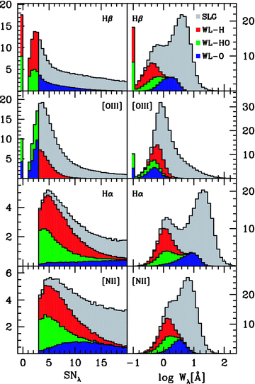
Histograms (in thousands of galaxies per bin) of emission-line signal-to-noise ratios (left) and equivalent widths (right) in the ELG sample. Red, green and blue regions correspond to WLGs of types H, HO and O, respectively, while SLGs are painted in grey. Non-detections (SN_λ < 1) are grouped in the first bin.

Open in new tabDownload slide

Importantly, as seen in the bottom panels of Fig. 2, WL-Hs are also among the sources in the low end of the [O iii], Hα and [N ii] equivalent width distributions, even though, by definition, SN_λ≥ 3 in all these lines. In the median, W_{[O iii]}= 0.7, W_Hα= 1.1 and W_{[N ii]}= 1.2 Å for WL-Hs. These galaxies thus have low W_λ in all major optical emission lines. Similar comments apply to WL-HOs. The requirement of SN_Hβ≥ 3 therefore biases SLG samples against objects whose emission lines in general have low W_λ. Equivalent widths are not considered in current emission-line classification schemes, but it is well known that low W_λ systems tend to avoid the tips of the AGN and SF wings in the BPT diagram. One thus expects to find few Seyferts and low metallicity SF galaxies among WL-Hs and WL-HOs.

The situation for WL-Os is somewhat different, in the sense that, as expected from the SN_{[O iii]} < 3 condition, they have low W_{[O iii]}, but the equivalent widths of other emission lines are not as small as those in WL-Hs and WL-HOs. For instance, the median W_Hα is about six times larger in WL-Os than in other WLGs, despite some overlap in the distributions (see the bottom right-hand panel in Fig. 2).

Given that SN_λ and W_λ are strongly coupled, one may wonder how important aperture effects are in shaping the WLG population. The fraction of WLGs over ELGs increases from ∼15 per cent at z= 0.024 to a little short of 60 per cent at z= 0.17. A naive interpretation of this trend is that as z increases more galaxy light enters the SDSS fibre, so nuclear emission lines become increasingly diluted and harder to detect. This suggests that, besides intrinsic line weakness, aperture effects play an important role in defining which galaxies have weak lines and which do not. While this effect is certainly present, it is heavily convolved with other potentially more important distance dependencies. Stellar masses, for instance, also grow strongly with z. We shall defer an analysis of these issues to a forthcoming paper.

4 ALTERNATIVE DIAGNOSTIC DIAGRAMS

The previous section has shown that WLGs comprise a large fraction of ELGs in the SDSS. Clearly, this numerous population deserves attention. We now look for ways to classify ELGs which include this usually forgotten population, trying to place WLGs in the framework of standard emission-line categories.

4.1 The BPT diagram

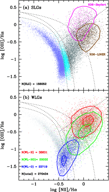
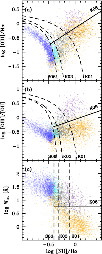
Fig. 3(a) shows the BPT diagram for the entire sample of SLGs defined in Section 2. As in all other diagnostic diagrams in this paper, for clarity purposes only one in every 10 galaxies is plotted, while the actual number of galaxies in each category which could have been plotted is given in the legend. None of the line ratios has been corrected for reddening, but their reddening dependence is negligible in the BPT. The curves show the SF/AGN border lines defined by S06, K03 and K01, and points are colour-coded accordingly. Points above the K01 line, often interpreted as ‘pure AGN’, are plotted in magenta or brown if they match the K06 criteria for Seyferts and LINERs, respectively. Points in black in this same region cannot be classified with their criteria due to the weakness of one or both of [O i] and [S ii] or due to conflict between the classifications obtained in different diagnostic diagrams (the ‘ambiguous’ category of K06). The straight line marks the Seyfert/LINER division line derived in Section 5.3, proposed to fix this ambiguity.

Figure 3

(a) The BPT diagram for SLGs. The dashed curves represent the SF/AGN division lines from S06, K03 and K01. Colours are used to indicate spectral classifications according to these lines. Magenta and brown points are Seyferts and LINERs according to the K06 criteria, and contours with these same colours correspond to a number density of 20 per cent of the peak value. The straight line is the Seyfert/LINER division line proposed in this paper (equation 10). (b) BPT diagram for WLGs, i.e. those where either or both of Hβ and [O iii] fail an SN_λ≥ 3 cut. Red, green and blue points and contours mark the location of WLGs of types WL-H (i.e. SN_Hβ < 3 and SN_{[O iii]}≥ 3), WL-HO (SN_Hβ and SN_{[O iii]} < 3) and WL-O (SN_Hβ≥ 3 and SN_{[O iii]} < 3), respectively. For reference, SLGs (the same as in panel a) are shown as the light grey points in the background. Contours correspond to number densities of 20 and 80 per cent of the peak density. Note that for clarity, in these and all other diagrams in this paper only one in every 10 galaxies is plotted. The actual numbers of galaxies in each category are listed in the lower left corner of the panels. N(total) is the number of SLG + WLG in the corresponding diagram.

Open in new tabDownload slide

Even though WLGs have (by definition) unreliable [O iii] and/or Hβ line intensities, it is instructive to estimate their location in the BPT diagram. This is done in Fig. 3(b), where we transgress the commonsense rule of using only good line measurements by plotting WL-H (in red), WL-HO (green) and WL-O (blue) sources. Contours with these same colours help tracing the location of these different types of WLGs in the BPT diagram. For reference, the background points represent the same SLGs as panel (a). Counting both SLGs and WLGs, panel (b) includes N(total) = 254 809 sources.

Given the small difference in wavelength between [O iii] and Hβ, the relation between SN_{[O iii]} and SN_Hβ should be similar to that between the [O iii] and Hβ fluxes, and thus one would expect WLGs of types H, HO and O to have [O iii]/Hβ > 1, ∼ 1 and < 1, respectively. These expectations are fully confirmed by Fig. 3(b). WL-Hs have and (median ± semi-interquartile range). They therefore lie within the region usually associated with ‘pure AGN’. Most of them sit on the lower side of the right wing, the realm of LINERs. WL-HOs have and ⁠, which place them well within the right wing, heavily overlapping with WL-H galaxies.

One should not be surprised to find that WL-Hs and WL-HOs are mostly AGN-like. Our definition of ELGs requires SN_λ≥ 3 in both Hα and [N ii], such that as one moves from the left to the right wing SN_Hα becomes the limiting factor. The median value of SN_Hα drops from 9 at to 4 for ⁠. With Hα so close to our SN_λ cut, and since F(Hβ) < F(Hα)/3, weak Hβ sources are bound to be found in the right wing.

While essentially no WL-H nor WL-HO galaxy falls in the SF region as defined by either K03 or S06, most WL-Os are consistent with an SF classification. They populate the bottom of the left wing, where the most massive and metal-rich SF galaxies are found (Asari et al. 2007; Stasińska et al. 2008). Although there is some overlap with WL-HOs, most WL-Os belong to the left wing, with 76 per cent of them having ⁠. This sets the bulk of these WLGs apart from type H and HOs, which are intrinsically right-wing sources.

While instructive, these results should be read with care, since dealing with low SN_λ lines involves important biases (e.g. Rola & Pelat 1994). Furthermore, as many as 28 per cent of our WLGs are not even plotted in Fig. 3 because of a missing Hβ or [O iii] measurement. One would therefore like to confirm these results with more robust alternative diagrams.

4.2 The BPTα diagram

One way to deal with a weak Hβ line is to replace it by a stronger hydrogen line, Hα. Fig. 4 shows the ‘BPTα’ diagram, whose horizontal axis is the same as in the BPT diagram but the vertical axis is [O iii]/Hα. Panel (a) shows SLGs (exactly the same ones appearing in Fig. 3a). WLGs are shown in panel (b), following the same colour coding as in Fig. 3(b). The dotted lines are the same as in Fig. 3(a), except for a 0.48 dex downwards shift corresponding to a dust-free case B Hα/Hβ ratio of 3.

Figure 4

The BPTα diagram: as the BPT, but replacing Hβ by Hα. Panels (a) and (b) are analogous to those in Fig. 3, except that in (b) the number of galaxies is larger because Hβ is not used. Note the downwards shift of the data points with respect to the dividing lines (the same as in Fig. 3 but shifted by − log 3) because of extinction.

Open in new tabDownload slide

As expected, the seagull shape is preserved in the BPTα diagram. The relative locations of WL-H, WL-HO and WL-O systems are also the same as in the original BPT plane, confirming the overall picture sketched above, namely that WL-H and WL-HO sources are mostly LINER-like right-wing sources, while WL-O systems behave like metal-rich SF galaxies. The advantage of this plot is twofold: first, WL-H systems have SN_λ≥ 3 in all three emission lines involved, and secondly, it allows the inclusion of 17 590 WLGs (19 per cent of the whole WLG population) absent from Fig. 3(b) because of lacking Hβ fluxes (non-detections, i.e. SN_Hβ < 1). However, even though in the case of WL-HOs the y-axis is more robust than in the BPT, this diagram does not solve the problem of low quality [O iii] fluxes, and thus the BPTα is not suitable to classify WL-Os and WL-HOs except in a statistical sense.

Unlike [O iii]/Hβ, the [O iii]/Hα ratio is sensitive to reddening. For a R_V=A_V/E(B−V) = 3.1 Cardelli, Clayton & Mathis (1989) law, 1 mag extinction in the V band increases [O iii]/Hβ by an insignificant 0.02 dex, but decreases [O iii]/Hα by 0.12 dex, causing detectable downward shifts in the BPTα plane. Such shifts can indeed be seen comparing Figs 3 and 4 and using the dividing lines as a reference. However, given that reddening correlates with other galaxy properties, both for SF and for AGN galaxies (Stasińska et al. 2004; K06), the BPTα diagram should still provide a meaningful diagnostic to separate ELGs into classes. This is confirmed by the clear separation of points of different colours in Fig. 4(a). In so far as classification is concerned, the most worrying class confusion caused by reddening occurs in the upper half of the right wing, where, because of their higher reddening (e.g. K06), Seyferts intrude into the zone occupied by LINERs, resulting in a substantial overlap (see the contours in Fig. 4a). Some confusion also occurs between SF and AGN when using the K01 line, but reddening causes little confusion of SF and AGN classes as defined by S06 and K03, given their nearly vertical dividing lines in the region corresponding to the body of the seagull.

4.3 The BPTo2 diagram

Another way to display galaxies with weak Hβ is to replace Hβ by [O ii] in the BPT diagram. As shown in Fig. 1, [O ii] is much less affected by low SN_λ than Hβ. To include [O ii] in the analysis, we momentarily modify our definition of ELGs by adding the requirement that SN_{[O ii]}≥ 3. This implies a 9 per cent reduction in the ELG sample as a whole, 2 per cent in the SLG sample and 24 per cent of WLGs as a whole, a modest price to pay in exchange for the replacement of a bad (or non-existent) datum by a convincing detection.

Fig. 5 shows the [O iii]/[O ii] versus [N ii]/Hα diagram (the same as in fig. 3 of BPT's paper, except for the order of the axes). Panel (a) shows galaxies with SN_λ≥ 3 in all four BPT lines and[O ii], while WLGs with SN_{[O ii]}≥ 3 are plotted in panel (b).

Figure 5

The BPTo2 diagram: [O iii]/[O ii] versus [N ii]/Hα. Analogous to Figs 3 and 4, but adding the requirement of SN_{[O ii]}≥ 3 to both SLGs and WLGs.

Open in new tabDownload slide

Like the BPT diagram, this ‘BPTo2’ diagram also opens up into SF and AGN wings. The main difference is that the right wing clearly splits into Seyfert and LINER branches, an effect which, although present, is much less pronounced in the BPT and BPTα planes. This split is evident in the contours corresponding to K06 Seyferts and LINERs (Fig. 5a), which, unlike in previous diagrams, do not overlap. The similarity of WL-H and W-HO sources is even more evident in terms of BPTo2 coordinates. Both types of WLGs populate the lower [O iii]/[O ii] branch of the right wing, where LINERs are located. A negligible number of WLGs intrude into the Seyfert branch, which is almost exclusively populated by SLGs.

Why does this diagram work so well? In this case, A_V= 1 mag implies an increase of [O iii]/[O ii] of 0.17 dex with respect to its intrinsic value. The enhanced distinction between Seyferts and LINERs seen in Fig. 5 is partly due to the fact that ionization state and reddening are positively correlated, i.e. Seyferts are more heavily reddened than LINERs (Ho, Filippenko & Sargent 2003; K06). Whereas in the BPTα plane this effect causes a certain degree of confusion of Seyferts and LINERs, in the BPTo2 it enhances the distinction between these two classes. Besides this extrinsic effect, [O iii]/[O ii] is more sensitive to the ionization state than [O iii]/Hβ, which also enhances the separation between Seyferts and LINERs. Moreover, [O ii] starts being collisionally de-excited at densities well below the critical density of [O iii], so a correlation between density and ionization state would cause a split in the [O iii]/[O ii] ratio. Since the narrow-line region of Seyferts is generally denser than that of LINERs (Ho et al. 2003), this could be yet another cause for the marked split seen in Fig. 5, although we note that this is a minor effect in our SDSS data, where Seyferts and LINERs span similar values of the density sensitive ratio of the 6731 to 6716 [S ii] lines. All these effects act in the same sense, explaining why the BPTo2 diagram is so effective in separating Seyferts from LINERs.

The gain in statistics with the BPTo2 diagram is significant, especially for WL-Hs, 83 per cent of which are in Fig. 5. All the data for this subset of objects now rely on convincing (SN_λ≥ 3) detections, greatly alleviating the problem of classification in the right wing. WL-Os are also well represented (83 per cent as well), while WL-HOs are present at a 56 per cent level, but in both cases the y-axis still contains uncertain [O iii] fluxes. Inevitably, the requirement of SN_{[O ii]}≥ 3 data makes the BPTo2 somewhat less inclusive than the BPTα diagram, but the difference is relatively small, and largely compensated by its much better Seyfert/LINER diagnostic power.

Neither the BPTα nor the BPTo2 allow a robust classification of WL-HOs and WL-Os. Due to the statistical power of the SDSS, diagrams utilizing SN_{[O iii]} < 3 data show an expected pattern, but individual objects cannot be reliably classified using such uncertain data. The next section presents an alternative which circumvents this limitation.

4.4 The EWαn2 diagram

The most economic way to classify galaxies is using just two lines. Hα and [N ii] are the best for this, both from the point of view of the number of galaxies that can be treated (Fig. 1) and from the point of view of the physical relevance of the line ratio. Miller et al. (2003), Brinchmann et al. (2004) and S06 have already argued for an SF/AGN classification using the [N ii]/Hα ratio only. However, such a classification does not allow one to distinguish Seyferts from LINERs.

We propose to use the equivalent width of Hα to break this degeneracy. This proposition entails a radical change in emission-line classification paradigm, in the sense that line ratios and equivalent widths measure different things. Emission-line ratios trace physical conditions in the ionized gas, while (neglecting escape of ionizing photons) W_Hα measures the power of the ionizing agent with respect to the optical output of the host's stellar population. One can justify this option on purely heuristic grounds: Seyfert galaxies are known to have higher values of W_Hα than LINERs, so why not use this to classify galaxies, especially when no other option is available?

Fig. 6 plots W_Hα versus [N ii]/Hα, the ‘EWαn2 diagram’. Its layout is like that of previous diagnostic diagrams, with SLGs on the top and WLGs on the bottom. This is the only diagram that allows us to plot all our 280 495 ELGs. Furthermore, by definition, only SN_λ≥ 3 data are used.

Figure 6

The EWαn2 diagram: W_Hα versus [N ii]/Hα. Colours and contours as in previous diagnostic diagrams. In panel (a) only galaxies with SN_λ≥ 3 in all BPT lines are plotted (SLGs), whereas in panel (b) the only requirement is that SN_λ≥ 3 in Hα and [N ii].

Open in new tabDownload slide

The SF/AGN diagnostic power of this diagram resides in the horizontal axis, while Seyferts and LINERs overlap in [N ii]/Hα, but are well separated in W_Hα (see also Fig. 7). As could be anticipated from the morphology of the BPT diagram, SF galaxies defined by either the S06 or the K03 criteria form nearly vertical boundaries in the EWαn2 diagram, and thus can be well separated in terms of [N ii]/Hα alone. In contrast, SF and AGN systems defined according to the K01 scheme are hopelessly mixed in this diagram, with substantial overlaps in both horizontal and vertical directions. For the reasons discussed in Section 5.1, this is neither surprising nor a serious drawback.

Figure 7

Distribution of W_Hα according to K01, K03, K06 and S06 spectral classes (bottom panels b, c and d) and WLG-type (top panel a). Panel (a) shows exclusively WLGs, whereas panels (b)–(d) are for SLGs. Panels (d) and (c) show results for the SF and AGN classes in K01, K03 and S06, while in panel (b) we show only K01-AGN and the Seyfert/LINER subdivision of K06. The dashed line in panel (a) corresponds to galaxies with SN_Hα≥ 3 but which are excluded from out ELG sample because SN_{[N ii]} < 3.

Open in new tabDownload slide

Turning to WLGs, Fig. 6(b) shows that, once again, WLGs of types H and HO overlap strongly with each other, occupying the region filled by LINERs in the SLG sample. As in other diagrams, WL-Os line up with the metal-rich (large [N ii]/Hα) SF galaxies, with a tail of objects stretching towards WL-Hs and WL-HOs.

Fig. 7 shows the distribution of W_Hα split by spectral class. Panel (d) shows the galaxies classified as SF according to the K01, K03 and S06 dividing lines on the BPT diagram, whereas panel (c) shows the corresponding AGN histograms. Panel (b) repeats the K01-AGN histogram, this time also showing the split into Seyfert and LINER sub-types according to the K06 scheme, which is based on seven emission lines and three diagnostic diagrams. (As already mentioned in Section 4.1, not all objects above the K01 line in the BPT diagram can be classified in the K06 Seyfert/LINER scheme, which explains why the magenta and brown lines do not add up to the black one.) All these panels are for SLGs only.

Panel (a) in Fig. 7 shows our WLGs, confirming that, despite some overlap, WL-Os have typical W_Hα values almost a full order of magnitude larger than WL-Hs and WL-HOs and that the latter two are indistinguishable in terms of W_Hα. The median ± semi-interquartile ranges of W_Hα are 6.7 ± 3.5, 1.1 ± 0.4 and 1.2 ± 0.6 Å for WL-O, WL-H and WL-HO, respectively. K06-LINERs in the SLG sample (Fig. 7b) have a W_Hα distribution which overlaps with those of WL-Hs and WL-HOs, but is skewed towards somewhat larger values: W_Hα= 2.2 ± 1.0 Å. This difference is most likely due to the more stringent requirements for a full K06 classification, which, by requiring good detections in many more lines, ends up skewing W_Hα towards larger values and indirectly excluding objects which are otherwise similar.

4.5 Summary

All the diagrams studied in this section point to the following.

• ELGs with weak Hβ and those with weak Hβ and [O iii] (WL-H and WL-HO) are predominantly LINERs.

• Part of the WL-HO population straddles the regions between bona fide LINERs and metal-rich SF galaxies in diagnostic diagrams. Objects in such intermediate locations are usually called ‘composite’ in current taxonomy.

• Galaxies with weak [O iii] (WL-O) are predominantly metal-rich SF galaxies, though some intrude into the LINER zone of diagnostic diagrams.

• Few WLGs are Seyferts.

Regarding the alternative diagnostic diagrams proposed in this section and their ability to rescue WLGs from the spectral classification ‘no man’s land', we have seen the following.

• Hβ can be replaced by Hα or by [O ii] without significant loss of classification power. This solves the problem of weak Hβ sources (about 41 per cent of all WLGs), which can all be appropriately classified on the basis of SN_λ≥ 3 lines exclusively.

• Seyferts and LINERs are much better distinguished in the BPTo2 diagram than in either the BPT or the BPTα.

• [N ii]/Hα does a reasonable job in separating SF from AGN as defined by S06 and K03, but does not separate K01-SF from K01-AGN.

• The equivalent width of Hα is the most economic way of distinguishing Seyferts from LINERs in the SDSS.

5 TRANSPOSITION OF STANDARD CLASSIFICATION SCHEMES TO OUR ALTERNATIVE DIAGRAMS

We have shown in the preceding section that a reasonably consistent emission-line classification of most SLGs and WLGs can be achieved in various diagnostic diagrams. We now convert these results into equations which allow one to transpose standard SF/AGN and Seyfert/LINER dividing lines to diagnostic diagrams other than those they were originally based on.

It is important to emphasize that the new dividing lines presented below are mere transpositions of other people's classification criteria. Specifically, we transpose the widely used K01, K03 and S06 SF/AGN border lines and the K06 Seyfert/LINER division to the more economic diagnostic diagrams discussed above. We are not therefore introducing independent classification schemes in a field where they already abound. This transformation is achieved with an adaptation of the optimal class separation technique of Strateva et al. (2001, see also Mateus et al. 2006). Although our main motivation is to provide practical criteria to classify WLGs, the results below are useful to ELGs in general.

Our objective transposition methodology does not overcome the limitations and ambiguities of spectral classification based on emission lines. Deficiencies in the reference classification schemes are propagated to the more widely applicable border lines derived below. Users of such classification schemes should be fully aware of such caveats. This is why, before presenting our results, we open a ‘parenthesis’ to ponder which of the three classification schemes studied here best reflects the fundamental distinction between SF and AGN galaxies in the BPT diagram.

5.1 Overtones of emission-line classification schemes

There has been some ambiguity, over the years, in the separation between SF and AGN galaxies in the BPT diagram. A now widely used scheme is to consider that all galaxies below the K03 line are ‘pure SF’ systems and all galaxies above the K01 line are ‘pure AGN’, while those in between are dubbed ‘composite’. This qualitatively plausible terminology is, however, misleading and inconsistent with both models and data.

The K01 line was originally designed to select, from a sample of galaxies, those that certainly harbour an active black hole. Their ‘extreme starburst’ line in the BPT plane was obtained by considering the upper envelope of model nebulae ionized by massive stars, considering a wide range of parameters and several stellar population synthesis models. Hence, according to the K01 models, sources currently classified as composites (i.e. between the K01 and K03 lines) do not require the presence of an AGN, and, conversely, locations above the ‘extreme starburst’ line may well be reached by composite SF+AGN systems. The K01 line in the BPT plane was never intended to trace the frontier of ‘pure AGN’, as it is used nowadays. On the contrary, its goal was to define a lower boundary for SF+AGN composites.

It is also fit to recall that photoionization models with either a pure AGN (Ferland & Netzer 1983; Halpern & Steiner 1983; Stasińska 1984) or a purely old stellar population (Stasińska et al. 2008) are able to cover the region between the K03 and K01 lines without mixing massive stars and AGN at all. From a more empirical point of view, stellar population studies (Schawinski et al. 2007; Cid Fernandes et al. 2009) show that galaxies with no ongoing star formation can populate this zone of the BPT diagram. Clearly, these systems are not truly SF+AGN composites.

All in all, the use of the term ‘composite’ to denote objects between the K01 and K03 lines is misleading, even if part of the galaxies in this zone is indeed mixtures of SF and AGN. If anything, such sources should be called ‘intermediate’, i.e. in between the bottom and the tip of the right wing.

Besides these interpretational issues, a more serious problem with the K01 line is that, as it became clear with the SDSS, real SF galaxies fall well below and to the left of it. In fact, the K01 line bears no resemblance whatsoever to any structure in the observational BPT. This mismatch prompted K03 to propose a dividing line more connected to the data. The K03 line was drawn empirically by simply displacing the K01 line in order to better trace the observed distribution of SF galaxies in the BPT diagram. This line runs a little higher than the upper envelope of the bulk of SF galaxies, and, more importantly, it is somewhat arbitrary at the bottom of the BPT diagram, which hosts a large proportion of SDSS galaxies. S06 produced a more stringent line which follows more closely the upper envelope of the bulk of SF galaxies and was extrapolated to the ‘body’ of the seagull, where the left and right wings meet and no clear frontier is seen. This extrapolation was achieved by means of photoionization models, and may obviously be wrong, but it is, for the moment, the best available.

We thus feel that the S06 divisory line between SF and AGN is better motivated than the K03 one, although, depending on the problem at hand, one might prefer using the K03 line, and for sources well within the right wing it makes no practical difference which of the two lines is used. On the other hand, because of its completely artificial shape in regard to the population of real galaxies in the BPT plane, the K01 SF/AGN division leads to different results and to an ill-defined classification of galaxies into various groups.

Because of it widespread use, we keep the K01 line in the analysis that follows, but the above considerations show that there are plenty of reasons to reconsider its role in the spectral classification of galaxies.

5.2 SF/AGN border lines in the BPTα and BPTo2 diagrams

We now start the transposition of classification criteria from BPT-based fiducial SF/AGN classification schemes. Three SF/AGN border lines are considered: K01, K03 and S06. All of these can be cast on to a single parametric form:

1

where and ⁠. These lines are drawn in Fig. 3, and the values of a, b and c are listed in Table 1. 3 We then consider other diagnostic diagrams and seek a dividing line y=f(x) which best maps the pre-defined BPT-based classification scheme on to the y×x plane of the new diagram.

Table 1

Open in new tab

Optimal y=a+b/(x+c) SF/AGN dividing lines.

Diagram	Line	y	x	a	b	c
BPT	K01	log [O iii]/Hβ	log [N ii]/Hα	1.19	0.61	−0.47	–	–	–	–	1
BPT	K03	log [O iii]/Hβ	log [N ii]/Hα	1.30	0.61	−0.05	–	–	–	–	1
BPT	S06	log [O iii]/Hβ	log [N ii]/Hα	0.96	0.29	+0.20	–	–	–	–	1
BPTα	K01	log [O iii]/Hα	log [N ii]/Hα	0.69	0.57	−0.38	0.98	0.94	0.99	0.92	0.84
BPTα	K03	log [O iii]/Hα	log [N ii]/Hα	0.68	0.49	+0.03	0.99	0.98	0.98	0.98	0.93
BPTα	S06	log [O iii]/Hα	log [N ii]/Hα	0.46	0.29	+0.22	0.98	0.98	0.98	0.99	0.93
BPTo2	K01	log [O iii]/[O ii]	log [N ii]/Hα	1.25	0.48	−0.21	0.93	0.91	0.98	0.91	0.80
BPTo2	K03	log [O iii]/[O ii]	log [N ii]/Hα	1.10	0.33	+0.11	0.97	0.93	0.96	0.96	0.84
BPTo2	S06	log [O iii]/[O ii]	log [N ii]/Hα	1.06	0.26	+0.24	0.97	0.94	0.93	0.98	0.83
EWαn2	K01	–	log [N ii]/Hα	−0.10	–	–	0.98	0.82	0.97	0.87	0.67
EWαn2	K03	–	log [N ii]/Hα	−0.32	–	–	0.97	0.91	0.95	0.95	0.79
EWαn2	S06	–	log [N ii]/Hα	−0.40	–	–	0.96	0.93	0.92	0.97	0.80

Diagram	Line	y	x	a	b	c
BPT	K01	log [O iii]/Hβ	log [N ii]/Hα	1.19	0.61	−0.47	–	–	–	–	1
BPT	K03	log [O iii]/Hβ	log [N ii]/Hα	1.30	0.61	−0.05	–	–	–	–	1
BPT	S06	log [O iii]/Hβ	log [N ii]/Hα	0.96	0.29	+0.20	–	–	–	–	1
BPTα	K01	log [O iii]/Hα	log [N ii]/Hα	0.69	0.57	−0.38	0.98	0.94	0.99	0.92	0.84
BPTα	K03	log [O iii]/Hα	log [N ii]/Hα	0.68	0.49	+0.03	0.99	0.98	0.98	0.98	0.93
BPTα	S06	log [O iii]/Hα	log [N ii]/Hα	0.46	0.29	+0.22	0.98	0.98	0.98	0.99	0.93
BPTo2	K01	log [O iii]/[O ii]	log [N ii]/Hα	1.25	0.48	−0.21	0.93	0.91	0.98	0.91	0.80
BPTo2	K03	log [O iii]/[O ii]	log [N ii]/Hα	1.10	0.33	+0.11	0.97	0.93	0.96	0.96	0.84
BPTo2	S06	log [O iii]/[O ii]	log [N ii]/Hα	1.06	0.26	+0.24	0.97	0.94	0.93	0.98	0.83
EWαn2	K01	–	log [N ii]/Hα	−0.10	–	–	0.98	0.82	0.97	0.87	0.67
EWαn2	K03	–	log [N ii]/Hα	−0.32	–	–	0.97	0.91	0.95	0.95	0.79
EWαn2	S06	–	log [N ii]/Hα	−0.40	–	–	0.96	0.93	0.92	0.97	0.80

Table 1

Open in new tab

Optimal y=a+b/(x+c) SF/AGN dividing lines.

Diagram	Line	y	x	a	b	c
BPT	K01	log [O iii]/Hβ	log [N ii]/Hα	1.19	0.61	−0.47	–	–	–	–	1
BPT	K03	log [O iii]/Hβ	log [N ii]/Hα	1.30	0.61	−0.05	–	–	–	–	1
BPT	S06	log [O iii]/Hβ	log [N ii]/Hα	0.96	0.29	+0.20	–	–	–	–	1
BPTα	K01	log [O iii]/Hα	log [N ii]/Hα	0.69	0.57	−0.38	0.98	0.94	0.99	0.92	0.84
BPTα	K03	log [O iii]/Hα	log [N ii]/Hα	0.68	0.49	+0.03	0.99	0.98	0.98	0.98	0.93
BPTα	S06	log [O iii]/Hα	log [N ii]/Hα	0.46	0.29	+0.22	0.98	0.98	0.98	0.99	0.93
BPTo2	K01	log [O iii]/[O ii]	log [N ii]/Hα	1.25	0.48	−0.21	0.93	0.91	0.98	0.91	0.80
BPTo2	K03	log [O iii]/[O ii]	log [N ii]/Hα	1.10	0.33	+0.11	0.97	0.93	0.96	0.96	0.84
BPTo2	S06	log [O iii]/[O ii]	log [N ii]/Hα	1.06	0.26	+0.24	0.97	0.94	0.93	0.98	0.83
EWαn2	K01	–	log [N ii]/Hα	−0.10	–	–	0.98	0.82	0.97	0.87	0.67
EWαn2	K03	–	log [N ii]/Hα	−0.32	–	–	0.97	0.91	0.95	0.95	0.79
EWαn2	S06	–	log [N ii]/Hα	−0.40	–	–	0.96	0.93	0.92	0.97	0.80

Diagram	Line	y	x	a	b	c
BPT	K01	log [O iii]/Hβ	log [N ii]/Hα	1.19	0.61	−0.47	–	–	–	–	1
BPT	K03	log [O iii]/Hβ	log [N ii]/Hα	1.30	0.61	−0.05	–	–	–	–	1
BPT	S06	log [O iii]/Hβ	log [N ii]/Hα	0.96	0.29	+0.20	–	–	–	–	1
BPTα	K01	log [O iii]/Hα	log [N ii]/Hα	0.69	0.57	−0.38	0.98	0.94	0.99	0.92	0.84
BPTα	K03	log [O iii]/Hα	log [N ii]/Hα	0.68	0.49	+0.03	0.99	0.98	0.98	0.98	0.93
BPTα	S06	log [O iii]/Hα	log [N ii]/Hα	0.46	0.29	+0.22	0.98	0.98	0.98	0.99	0.93
BPTo2	K01	log [O iii]/[O ii]	log [N ii]/Hα	1.25	0.48	−0.21	0.93	0.91	0.98	0.91	0.80
BPTo2	K03	log [O iii]/[O ii]	log [N ii]/Hα	1.10	0.33	+0.11	0.97	0.93	0.96	0.96	0.84
BPTo2	S06	log [O iii]/[O ii]	log [N ii]/Hα	1.06	0.26	+0.24	0.97	0.94	0.93	0.98	0.83
EWαn2	K01	–	log [N ii]/Hα	−0.10	–	–	0.98	0.82	0.97	0.87	0.67
EWαn2	K03	–	log [N ii]/Hα	−0.32	–	–	0.97	0.91	0.95	0.95	0.79
EWαn2	S06	–	log [N ii]/Hα	−0.40	–	–	0.96	0.93	0.92	0.97	0.80

For example, to separate left- and right-wing galaxies in the BPTα diagram (Fig. 4) we use equation (1) with and ⁠, tagging points below and above this line as SF and AGN, respectively, and search for values of a, b and c which best reproduce the SF/AGN classification scheme of, say, S06. This optimization is achieved by identifying the coefficients a, b and c which maximize the product (⁠⁠) of completeness (⁠⁠) and reliability (⁠⁠) fractions:

2

where is the fraction of galaxies classified as SF according to the original line, say S06, which are correctly classified as such by our new dividing line, and is the fraction of objects below the new y=f(x) line which are also S06-SF, while and are the corresponding completeness and reliability fractions for AGN, respectively. Except for strong covariances among a, b and c, which require some numerical care but are irrelevant for the purposes of identifying an effective dividing line, this is a straightforward procedure to translate a well-established classification criterion to an alternative one.

The same procedure is applied to the BPTo2 diagram. The results are summarized in Table 1, which lists the meaning of y and x, and the values of a, b and c for the BPTα and BPTo2 diagrams, for which SF/AGN dividing lines in the form of equation (1) are suitable. The resulting transformations are very efficient, with completeness (⁠⁠) and reliability (⁠⁠) factors ranging from 91 to 99 per cent (Table 1).

Figs 8(a) and (b) show as dashed lines the transposed S06, K03 and K01 SF/AGN boundaries in the BPTα and BPTo2 diagrams. In both diagrams, the transposed S06 and K03 lines yield slightly better results (higher ⁠) than K01. This happens for the already noted reason that the S06 and K03 lines intercept the data at more vertical angles than the K01 one, being therefore less prone to reddening effects, which act vertically in both the BPTα and BPTo2 diagrams.

Figure 8

BPTα (a), BPTo2 (b) and EWαn2 (c) diagnostic diagrams, showing the transposed SF/AGN border lines of S06, K03 and K01 in dashed lines. Solid lines show the transposed Seyfert/LINER classification of K06 (see Section 5.6 for the corresponding equations). SLGs are plotted following the same colour-coding of Fig. 3(a). WLGs are plotted in orange.

Open in new tabDownload slide

5.3 Parameters for Seyfert/LINER border lines in the BPT, BPTα and BPTo2 diagrams

K06 performed a detailed study of right-wing sources in the SDSS, which lead them to propose a new set of criteria to tell Seyferts from LINERs. These criteria are based on an empirical mapping of the bimodality observed in the [O iii]/Hβ versus [O i]/Hα and [S ii]/Hα diagrams for objects with SN_λ≥ 3 (also visible in the BPT, but less clearly so), where AGN bifurcate into Seyfert and LINER branches. After filtering out SF and putative SF+AGN composites by requiring objects to lie above the K01 extreme starburst lines in the BPT, [O i]/Hα and [S ii]/Hα diagrams, they define Seyferts and LINERs using linear division lines in the versus and versus spaces.

This scheme has a couple of caveats. First, as is common with classification schemes involving more than one diagnostic diagram, inconsistencies abound. In this particular case, galaxies with ambiguous classification are as numerous as properly classified Seyferts and LINERs. A second drawback of the K06 scheme is that, as seen in Fig. 1, it requires far more good quality emission-line data than one can usually afford with SDSS-like spectra.

The technique explained above offers an opportunity to remedy this situation, translating the K06 classification scheme into simpler, more economic and thus more widely applicable criteria.

We start deriving a Seyfert/LINER classification criterion based exclusively on the BPT diagram. We compute the values of the coefficients of a simple straight line in the BPT plane which maximize the product ⁠, where ⁠) is the fraction of K06-Seyfert (LINER) galaxies which are correctly classified as such by our dividing line and ⁠) is the fraction of objects above (below) our line which are also Seyfert (LINER) according to K06. Sources with an ambiguous classification are not used in this transposition. We find that a border line

3

does a good job in translating the K06 Seyfert/LINER classification to the BPT diagram, with completeness and reliability fractions of 92 per cent or better (Table 2). This line is drawn in Fig. 3. Our derived parameters are very similar to the a= 1.05 and b= 0.45 adopted by Schawinski et al. (2007).

Table 2

Open in new tab

Optimal y=a x+b Seyfert/LINER dividing lines.

Diagram	y	x	a	b
BPT	log [O iii]/Hβ	log [N ii]/Hα	1.01	0.48	0.95	0.92	0.95	0.93	0.77
BPTα	log [O iii]/Hα	log [N ii]/Hα	1.20	−0.15	0.91	0.85	0.90	0.85	0.59
BPTo2	log [O iii]/[O ii]	log [N ii]/Hα	0.64	−0.06	0.98	0.96	0.98	0.97	0.88
EWαn2	WHα	–	–	6 Å	0.91	0.85	0.90	0.86	0.60

Diagram	y	x	a	b
BPT	log [O iii]/Hβ	log [N ii]/Hα	1.01	0.48	0.95	0.92	0.95	0.93	0.77
BPTα	log [O iii]/Hα	log [N ii]/Hα	1.20	−0.15	0.91	0.85	0.90	0.85	0.59
BPTo2	log [O iii]/[O ii]	log [N ii]/Hα	0.64	−0.06	0.98	0.96	0.98	0.97	0.88
EWαn2	WHα	–	–	6 Å	0.91	0.85	0.90	0.86	0.60

Table 2

Open in new tab

Optimal y=a x+b Seyfert/LINER dividing lines.

Diagram	y	x	a	b
BPT	log [O iii]/Hβ	log [N ii]/Hα	1.01	0.48	0.95	0.92	0.95	0.93	0.77
BPTα	log [O iii]/Hα	log [N ii]/Hα	1.20	−0.15	0.91	0.85	0.90	0.85	0.59
BPTo2	log [O iii]/[O ii]	log [N ii]/Hα	0.64	−0.06	0.98	0.96	0.98	0.97	0.88
EWαn2	WHα	–	–	6 Å	0.91	0.85	0.90	0.86	0.60

Diagram	y	x	a	b
BPT	log [O iii]/Hβ	log [N ii]/Hα	1.01	0.48	0.95	0.92	0.95	0.93	0.77
BPTα	log [O iii]/Hα	log [N ii]/Hα	1.20	−0.15	0.91	0.85	0.90	0.85	0.59
BPTo2	log [O iii]/[O ii]	log [N ii]/Hα	0.64	−0.06	0.98	0.96	0.98	0.97	0.88
EWαn2	WHα	–	–	6 Å	0.91	0.85	0.90	0.86	0.60

The same transposition procedure was carried out for the BPTα and BPTo2 diagrams, with results shown as solid lines in panels (a) and (b) of Fig. 8. As for the BPT diagram, a simple y=ax+b border line suffices to separate Seyferts from LINERs in these diagrams.

Table 2 lists the optimal values of a and b for the BPT, BPTα and BPTo2 diagrams. As in the case of the SF/AGN classification, the quality of these transformations can be measured by the completeness and reliability factors, which range from 85 to 98 per cent (Table 2). The best results are achieved for the BPTo2 diagram (⁠⁠), followed by the BPT (0.77) and BPTα (0.59), corroborating the qualitative assessment of the Seyfert/LINER diagnostic power of these diagrams presented in Section 4.

The addition of WLGs to the BPT and BPTα diagrams causes significant dilution of the Seyfert/LINER dichotomy, leading to the nagging suspicion that selection effects might be behind what is presumed to be a physical class-separation. The fact that the bimodality is present in the BPTo2 plane (Fig. 8b) should dismiss such worries. The inclusion of WLGs, however, does lead to a new perspective on the Seyfert/LINER bimodality, as discussed in Section 6.3.

5.4 Comments on combinations of Seyfert/LINER and SF/AGN criteria

Accepting that AGN come in either Seyfert or LINER flavours, one is led to a classification scheme based on three fundamental classes: SF galaxies, Seyferts and LINERs. Complementing the S06 SF/AGN classification with the Seyfert/LINER division schemes derived above thus leads to S06-SF, S06-Seyferts and S06-LINERs, and similarly for K03 and K01.

A caveat with these combinations is that our Seyfert/LINER dividing lines were calibrated exclusively on the basis of the K06 criteria, which in turn were defined only for K01-AGN, and thus comprise just a subset of S06 and K03-AGN. We have expressed strong reservations with regard to the K01 SF/AGN scheme (Section 5.1), but these reservations do not extend to the K06 Seyfert/LINER classification scheme, which is rooted on empirical evidence of a bimodality in emission-line diagnostic diagrams for SLGs. None the less, rigorously speaking, the K06 Seyfert/LINER division applies only to K01-AGN, and extending it to S06 and K03 involves an extrapolation to intermediate zones in diagnostic diagrams, where the bimodality becomes fuzzier.

As can be seen in the BPT (Fig. 3), BPTα (Fig. 8a) and BPTo2, (Fig. 8b), the extrapolated Seyfert/LINER demarcation lines do not cut the right wing in equal halves. Sources on the LINER side of these lines become more common considering the whole population than when restricting to galaxies above the K01 line.

5.5 Dividing lines in the EWαn2 diagram

A simpler transposition strategy was used to deal with the EWαn2 diagram. As discussed in Section 4.4 and shown in Fig. 6, the SF/AGN diagnostic power in this case lies almost exclusively on the horizontal axis, while the differentiation of Seyferts and LINERs occurs in the vertical direction. Fitting y(x) dividing lines to this diagram would thus be an exaggeration, given this one-dimensional behaviour. Apart from this simplification, the same optimal separator technique described above was used to identify class separation boundaries.

The division of SFs and AGN according to the S06 BPT-based scheme is best transposed to ⁠, while the optimal boundary for the K03 division is ⁠. As anticipated (Fig. 6), the least satisfactory results are obtained for the K01 line, whose formally best division at misclassifies about 18 per cent of the Seyferts.

The separation of Seyfert and LINER classes as defined by K06 is best accomplished setting a boundary at W_Hα= 6.0 Å, in agreement with the histograms in Fig. 7. The completeness and reliability fractions are marginally better than for the BPTα, but smaller than for the BPT and BPTo2 diagrams (Table 2).

Overall, compared to standard diagnostic diagrams, the EWαn2 diagram offers an attractive compromise between classification efficiency and economical aspects.

Fig. 9 shows the location of galaxies below (panel a) and above (panel b) the W_Hα= 6 Å threshold in our alternative BPTo2 diagram for sources where [O ii], [O iii], Hα and [N ii] are all detected with SN_λ≥ 3. The plot shows that most sources in the K01-LINERs region of this diagram, i.e. those in the bottom-right ‘corner’ below the K06 line and to the right of the K01 line, indeed have W_Hα < 6 Å (points in black in panel b and in light grey in panel a). Similarly, the zone corresponding to K01-Seyferts is populated predominantly by galaxies with W_Hα > 6 Å. This consistency is expected, since the K06 criteria were used to calibrate the border lines in both diagrams. Note that W_Hα < 6 Å also eliminates nearly all S06 and K03 SF systems, even though this criterion was not explicitly designed to do so. In the intermediate zone between the K01 line and the S06 lines, sources with W_Hα below and above the 6 Å cut become heavily mixed. The extrapolation of the K06-based division line in the BPTo2 plane places most such intermediate sources in the LINER branch, while the W_Hα cut suggests a more even mix of Seyferts and LINERs.

Figure 9

BPTo2 diagram indicating with black points the location of galaxies below (a) and above (b) the optimal separation Seyfert/LINER separation in terms of the equivalent width of Hα: W_Hα= 6.0 Å. Points in violet and black mark S06-SF and S06-AGN according to the and ≥−0.40 criteria, respectively. For reference, the background points (light grey) show all galaxies, irrespective of W_Hα. Only SN_λ≥ 3 data (in [O ii], [O iii], Hα and [N ii]) are used in these plots. The dividing lines are the same as in Fig. 8(b) (equations 5, 7, 9 and 12).

Open in new tabDownload slide

5.6 Summary of SF/AGN and Seyfert/LINER dividing lines

For ease of use, we open up the results summarized in Tables 1 and 2 into explicit equations for emission-line classification (shown in Fig. 8).

The S06, K03 and K01 SF/AGN dividing lines in the BPT plane are best transposed to the BPTα and BPTo2 diagrams through

4

5

6

7

8

9

An alternative (and cheaper) way to distinguish SF from AGN is through the [N ii]/Hα ratio. The limiting values are and −0.10 for the S06, K03 and K01 SF/AGN schemes, respectively. Recall that, for the reasons discussed in Section 5.1, the K01 classification scheme is misleading, and thus equations (8), (9) and the criteria are not recommended.

The K06 Seyfert/LINER classification scheme can be recast on to dividing lines in the BPT, BPTα and BPTo2 diagrams by

10

11

12

of which the last one (BPTo2) is the most recommended.

In the absence of reliable [O iii] and [O ii] fluxes, W_Hα does an acceptable job in distinguishing Seyferts from LINERs, with an optimal border line located at W_Hα= 6 Å.

6 THE ELG POPULATION IN LIGHT OF OUR ALTERNATIVE CLASSIFICATION

With the alternative and more inclusive classification schemes outlined above, we can finally place WLGs on to standard spectral categories and abandon the WL-H, WL-HO and WL-O notation. This is the topic of this section, which also discusses how the inclusion of this population changes the balance of galaxy spectral classes in the nearby Universe and how WLGs affect the dichotomy between Seyferts and LINERs.

The three classes considered below are SF, Seyferts and LINERs, respectively. Given our comments on the meaning of the S06, K03 and K01 divisory lines (see Section 5.1), we intentionally do not define a class of ‘composite’ galaxies, even though such systems are expected to be present in the SDSS. The K01 scheme is not capable of adequately confining such SF+AGN hybrids in any of the three classes. Ad hoc combinations of criteria, such as K01+K03, can be postulated to select sources with intermediate line ratios, but these are not necessarily true mixtures of SF and AGN-powered emission-line systems. The situation is less confusing with the S06 scheme, where the SF class is designed to isolate ‘pure SF’ systems, and hence SF+AGN hybrids are confined to S06-Seyferts or S06-LINERs. The same applies to the K03 scheme, which, according to the hybrid photoionization models by S06, admits AGN contributions to the ionizing power of at most 3 per cent. In both these schemes, anything that is not a pure SF counts either as a Seyfert or as a LINER. This is the best that can be done, given that unambiguous definitions of ‘pure AGN’, SF+AGN composites and other mechanisms leading to AGN-like line ratios are not possible on the basis of optical emission-line data alone.

6.1 Classification of WLGs

Fig. 10 shows the results of the classification of WLGs into SF, Seyfert and LINER classes using the BPTα (top), BPTo2 (middle) and EWαn2 (bottom) diagrams. For the distinction between AGN and SF galaxies, the left-hand panels use the divisory lines derived by transposing the S06 criterion, while the middle and right-hand panels show results obtained with the K03 and K01 criteria, respectively.

Figure 10

Spectral classification of WLGs according to the BPTα (top row), BPTo2 (middle) and EWαn2 (bottom) diagrams. Results for the S06, K03 and K01 classification schemes are given in the left-hand, middle and right-hand panels, respectively. For each diagram, only galaxies with SN_λ≥ 3 in all lines involved are classified. In the BPTo2, WL-H^★ denotes WL-Hs which have SN_{[O ii]}≥ 3.

Open in new tabDownload slide

With the BPTα diagram, WLG galaxies can be robustly classified only if they belong to the WL-H family, so only those are represented in the top panels in Fig. 10. As clearly seen in this figure, most WL-Hs are LINER-like, whatever the system of divisory lines is used (S06, K03 or K01). In the K01 system, 14 per cent of WL-Hs cross the border towards the SF zone, but, as already explained, these are definitely not pure SF galaxies. The tiny numbers of S06-SF and K03-SF among WL-Hs indicate that almost all of them are indeed AGN-like.

For the BPTo2 diagram (middle panels), only galaxies with SN_λ≥ 3 in [O ii], [O iii], Hα and [N ii] are included to ensure a robust classification. Here again we see that most WL-Hs are classified as AGN, and most of them are LINER-like. As noted before (see Fig. 5), the BPTo2 diagram is much more efficient than both the BPT and the BPTα diagrams in distinguishing Seyferts from LINERs. About 90 per cent of WL-Hs are S06-LINERs and only a tiny proportion is S06-Seyferts. Similar fractions apply to K03.

The bottom panels of Fig. 10 show the results obtained with the EWαn2 diagram. This time, we can also classify galaxies from the WL-O and WL-HO families, whose numbers are represented by hatched and empty areas, respectively. Adding these new sources further increases the number of LINER-like galaxies in the S06 and K03 schemes. The K01 scheme shows a different picture, dividing the WLGs almost equally among SFs and LINERs, but, as emphasized before (see Fig. 8), the EWαn2 diagram is not suitable to tell K01-SF from K01-AGN. The weak line SF galaxies identified with the S06 and K03 schemes, on the other hand, are pure SF galaxies. They come mostly from the WL-Os, robustly classifiable in the EWαn2 diagram but not in previous ones. About 53 per cent of WL-Os turn out to be SF galaxies according to the K03 scheme, a fraction which reduces to 29 per cent in the more stringent S06 scheme.

6.2 A revised census of ELGs in the local Universe

We are now able to classify a significantly larger number of galaxies than when using the BPT diagram: from ∼20 to 50 per cent more, depending on the alternative diagram that is used. Does this change our view of the population of ELGs in the local Universe?

In order to have a reference for comparison, we show in Fig. 11 the result of the classification of our SLG sample into SF-, Seyfert- and LINER-like classes using the BPT diagram and the S06 (left), K03 (middle) and K01 (right) divisory lines. The relative populations of SF/Seyferts/LINERs in our SLG sample are, in percentages, 44/6/50 (S06 scheme), 60/6/34 (K03) and 84/5/11 (K01), respectively. Thus, LINERs represent half of the total population of SLGs when using the S06 scheme and about one-third when using the K03 one. This large difference for such apparently equivalent classification schemes stems from the large number of sources in the geometrically small space between the S06 and K06 lines in the BPT diagram. The K01 scheme gives a vast majority of SF galaxies, but whereas in the S06 and K03 schemes the SF class is meant to represent ‘pure SF’, K01-SFs include everything below their ‘extreme starburst’ line, whose meaning has been questioned above. Obviously, these differences must be kept in mind when comparing numbers of galaxies derived under different schemes.

Figure 11

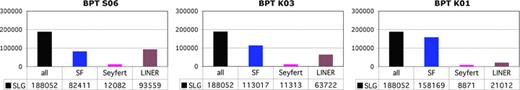
Emission-line classification according to purely BPT-based criteria. Left, middle and right plots correspond to results obtained with the S06, K03 and K01 criteria, respectively. Only SN_λ≥ 3 lines are used, which in this case correspond to our definition of SLGs.

Open in new tabDownload slide

Fig. 12 shows the distribution among SF, Seyferts and LINERs of all the galaxies whose emission-line intensities allow a decent (SN_λ≥ 3) classification in the BPTα, BPTo2 or EWαn2 diagram. As in the previous figures, S06, K03 and K01 classifications are shown separately.

Figure 12

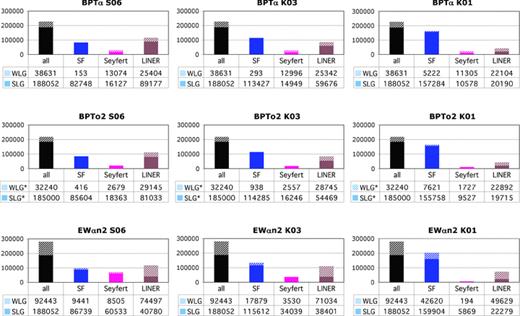
As Fig. 10, but now including both SLGs and WLGs to provide a global census of ELG classes in the SDSS.

Open in new tabDownload slide

By using the BPTα (top panels) instead of the BPT, we are able to add 21 per cent more objects to our census. SLGs are plotted as filled areas, while WL-Hs are represented by hatched areas. As expected, these WLGs do not increase much the SF population (except in the K01 scheme), but they significantly increase the Seyfert and LINER populations. The BPTo2 diagram (middle panels in Fig. 12) adds 17 per cent more galaxies with respect to those classifiable in the BPT. The partitioning is similar to that obtained with the BPTα diagram, except for a somewhat smaller proportion of Seyferts. Whereas in the BPTα diagram weak line Seyferts make up between 45 (S06) and 52 per cent (K01) of the total WLG + SLG Seyfert population, in the BPTo2 this fraction is between 13 and 15 per cent. Given the higher Seyfert/LINER diagnostic power of the BPTo2, we favour the latter results, which corroborate the view that few WLGs have Seyfert-like emission lines. In both diagrams, the K01 scheme is the one for which WLGs most increase the population of LINERs (by 52 per cent in the BPTα and 54 per cent in the BPTo2). The implication is that, under the widespread view that the K01 criteria isolate ‘pure AGN’, a full half of the ‘pure-LINER’ population is completely missed by imposing a standard SN_λ≥ 3 quality control on the BPT lines.

As a whole, classifications derived with the BPTα and BPTo2 diagrams do not change drastically the balance of SF, Seyfert and LINER galaxies. For instance, in the S06 scheme, the SF/Seyfert/LINER percentages change from 44/6/50 with the BPT to 37/13/50 (BPTα) and 40/10/50 (BPTo2).

Larger differences are obtained classifying galaxies with the EWαn2 diagram, specially for the S06 and K01 schemes, which yield 34/25/41 and 72/2/26 percentage SF/Seyfert/LINER proportions. The large fraction of S06-Seyferts comes mostly from the W_Hα > 6 Å objects close to the frontier, whose Hα emission is likely contaminated (if not dominated) by star formation (see also Fig. 9). In the K01 scheme, the increase in the LINERs' share is essentially due to WLGs, while the miniscule fraction of Seyferts is due to the fact that the frontier is a rather inefficient translation of the K01 SF/AGN criteria. In the K03 scheme, on the other hand, the changes in the SF/Seyfert/LINER classes deduced from the EWαn2 diagram are not as large. The inferred proportions are 48/13/39, compared to 60/6/34 deduced with the BPT.

A general result which is immune to the subtleties associated with all these comparisons is that, in all diagrams and for all classification schemes, LINERs are the ones which grow the most in absolute numbers with the inclusion of WLGs. This is also the class which grows the most in relative terms in the two diagrams most apt to distinguish AGN sub-types: the BPTo2 and EWαn2.

It seems to us that, for practical purposes, the EWαn2 classification is more convenient, not only because it allows one to increase by about 50 per cent the number of galaxies that can be classified, but also because it considers the strength of the AGN with respect to its host galaxy as a parameter that is more important than the ionization state of the gas to distinguish between strong and weak AGN.

6.3 The Seyfert/LINER dichotomy revisited

The Seyfert/LINER classification criteria proposed in this paper simply transpose the bimodality identified by K06 to our more economic diagnostic diagrams. Given that the stringent requirements on data quality imposed by K06 completely exclude the huge population of AGN-like WLGs, it is fit to ask: does the Seyfert/LINER dichotomy subsist when WLGs are considered?

A visually convenient way to inspect bimodality effects on our diagnostic diagrams is to swap the order of the axis and count sources as a function of x for a fixed ⁠. This is done in Figs 13(a)–(c) for the BPT, BPTo2 and EWαn2 diagrams, respectively. The top panels show the inverted diagrams, colour coding S06-SF, S06-Seyferts and S06-LINERs by violet, magenta and brown points, respectively. Horizontal lines mark a 0.07 dex wide window around y=− 0.02, chosen for illustration purposes. Histograms of SLGs (blue), WLGs (red) and all ELGs (black) along this narrow strip are presented in the second panel from the top, while the bottom panels show the corresponding median equivalent width and signal-to-noise ratio of Hβ, and the [O iii] luminosity as a function of x.

Figure 13

A different look at the Seyfert/LINER bimodality in diagnostic diagrams. The top panels in columns (a), (b) and (c) show the BPT, BPTo2 and EWαn2 diagrams, respectively, but with on the y-axis. Violet, brown and magenta points correspond to SF, Seyferts and LINERs, respectively, as classified with the S06 scheme. The second panel from the top shows histograms of x-values for SLGs (blue), WLGs (red) and all ELGs (black) galaxies within the narrow strip in marked in the top panel. Dotted vertical line marks the x-value associated with the centre of the selected y-range on the corresponding Seyfert/LINER divisory line. In all cases, this coincides with a shoulder in the SLG histograms. The bottom panels show the median value of the equivalent width and signal-to-noise ratio of Hβ, and the [O iii] luminosity, separated in SLGs, WLGs and all ELGs. Panels (d) and (e) are like panels (a) and (b) but applying translations and rotations to the BPT and BPTo2 diagrams. The transformations from the original coordinates to the new ones (x′, y′) is such that (i) the origin is centred at the intersection of the S06 SF/AGN and Seyfert/LINER divisory lines and (ii) the Seyfert/LINER line becomes vertical (x′= 0). This rotation ensures that the narrow strips in y′ (marked in the top panels) cross the Seyfert/LINER line perpendicularly, facilitating the visualization of the bimodalities.

Open in new tabDownload slide

In the BPT diagram (Fig. 13a), the distribution of SLGs presents a clear shoulder at ⁠, exactly the value corresponding to the transition from LINERs to Seyferts for in equation (10) (marked by a vertical dotted line). This evidence for a bimodality disappears when WLGs are included, as shown by the black histogram. The W_Hβ and SN_Hβ panels show that the Seyfert/LINER frontier coincides with the region where Hβ is the weakest, and thus also where restrictions upon SN_Hβ have a larger impact. Does this mean that there is a continuum of emission-line properties between Seyferts and LINERs when considering a more complete sample of galaxies than SLGs, and that there is no dichotomy?

It does not seem to be the case. In the BPTo2 diagram (Fig. 13b), the Seyfert/LINER bimodality survives the inclusion of WLGs. Again, SLGs have a shoulder in the distribution of x-values starting at the value of [O iii]/[O ii] expected from our transposed version of the K06 Seyfert/LINER classification (equation 12). As in the BPT, WLGs approximately double the low x (⁠ in this case) counts, but this time they do not wash away the change in the distribution as one goes from LINERs to Seyferts. The histograms for the EWαn2 diagram (Fig. 13c) also show evidence for two populations, with a high W_Hα hump starting precisely at our proposed Seyfert/LINER frontier: W_Hα= 6 Å.

Figs 13(d) and (e) show two further experiments with the BPT and BPTo2 diagrams, respectively. The top panels show these diagrams after translation and rotation operations. The transformations from the original coordinates to the new ones (x′, y′) are such that (i) the origin is centred at the intersection of the SF/AGN and Seyfert/LINER divisory lines and (ii) the Seyfert/LINER line becomes vertical (x′= 0). This allows us to count galaxies across a y′-strip which crosses our Seyfert/LINER frontiers at right angles, facilitating the visualization of bimodalities. Indeed, unlike with the original coordinates, the histograms for SLGs now show two modes, particularly strong in the BPTo2. These alternative representations of the data confirm that the bimodality in the BPT appears only for SLGs, whereas in the BPTo2 it cannot be attributed to a selection effect. Interestingly, the W_Hβ, SN_Hβ and L_{[O iii]} profiles become essentially flat for x′ < 0 (corresponding to LINERs), signalling a transition to a different regime.

These results suggest that there are, indeed, at least two classes of AGN-like galaxies. K06 speculate that this dual behaviour is analogous to the high and low states of black hole accretion in X-ray binaries, i.e. two regimes of the same physical process. A different possibility is that the bimodality in emission-line properties originates from two completely different sources of ionizing radiation: an active nucleus versus old stars. As shown by Stasińska et al. (2008), many SDSS galaxies belonging to the LINER zone in the BPT diagram have an old stellar population whose ionizing photons alone are able to produce the observed emission-line intensities. These ‘retired galaxies’ are erroneously counted as AGN, leading to the illusion of a dichotomy in the AGN population. It might therefore be that the real dichotomy is between AGN and retired galaxies, and not between two states of black hole accretion. A more detailed assessment of this scenario is postponed to a forthcoming communication.

7 SUMMARY AND CONCLUSION

This paper revisited the emission-line classification of galaxies, focusing on the numerous population of galaxies which are often left out of emission-line studies because of their weak (low signal-to-noise ratio) lines. We have shown that WLGs, defined as systems in which both Hα and [N ii] have ≥3σ detections but where either or both of Hβ and [O iii] is weaker, amount to about one in three ELGs in the SDSS DR7. This already large fraction increases nearly twofold if one concentrates on the right wing of the [O iii]/Hβ versus [N ii]/Hα BPT diagram, where ionizing sources other than young stars have a significant impact on integrated emission-line properties. The lack of good quality data leaves these objects in a classification limbo, preventing a complete census of the population of galaxies with emission lines.

In order to rescue WLGs from their uncertain place in current emission-line classification schemes, we have investigated alternative diagnostic diagrams, all of which keep [N ii]/Hα as a horizontal axis, but where Hβ is replaced by a stronger line (Hα or [O ii]) or where the ionization-level sensitive [O iii]/Hβ ratio is replaced by the equivalent width of Hα. The classification power of these ‘cheaper’ alternative diagrams was evaluated from the location of well-classified, strong line sources in these same diagrams.

To avoid introducing further entropy in the emission-line taxonomy of galaxies, SF/AGN and Seyfert/LINER border lines in these diagrams were traced by means of an objective method devised to transpose popular classification schemes (K01, K03, S06 and K06) in an optimal way. We find that the BPTα (Fig. 4) and BPTo2 (Fig. 5) diagrams do an excellent job in placing galaxies with weak Hβ but strong [O iii] in standard SF/AGN and Seyfert/LINER categories. In particular, the BPTo2 has the ability of mimicking with exquisitely high efficiency the detailed Seyfert/LINER classification of K06, but at a much reduced cost in terms of data quality requirements.

The most economic classification is achieved with the EWαn2 diagram (W_Hα versus [N ii]/Hα), where SF and AGN are segregated in terms of [N ii]/Hα, while Seyferts and LINERs differ in the vertical axis, with an optimal class division at W_Hα= 6 Å. Inevitably, the correspondence with standard classification schemes is not as good as for diagrams involving more data, but the cost/benefit is such that it is tempting to propose it as a fundamental classification scheme. This is the only scheme able to classify all galaxies with 3σ or better detection of Hα and [N ii], which comprise approximately three-quarters of the galaxies in the SDSS.

Working definitions were proposed to identify which of Hβ and/or [O iii] prevents a full BPT-based classification, leading to the weak Hβ but strong [O iii] (WL-H), weak [O iii] but strong Hβ (WL-O), and weak Hβ and [O iii] (WL-HO) sub-divisions. WL-H and WL-HO sources share many emission-line properties which indicate their predominantly LINER-like nature. WL-Os, on the other hand, are best described as SF systems whose [O iii] flux is suppressed by enhanced nebular cooling associated with high metallicity. Some of them, however, mingle amongst WL-H and WL-HOs, and thus probably have an AGN-like component.

Our WLG-rescuing operation leads to a revision of the partition of galaxies in the nearby Universe into different spectral types in the sense that metal-rich SF galaxies and especially LINERs occur more often than would be deduced by ignoring WLGs.

While adapting currently popular schemes to distinguish SF galaxies from AGN we have stumbled upon known, but widely overlooked, inconsistencies. The most worrying of these is the way that the K01 ‘extreme starburst’ line in the BPT diagram is currently used to isolate ‘pure AGN’. This line was never designed to do this neither is it capable of doing so in more than a qualitative sense. Similarly, and contrary to current practice, using the K01 line as an upper bound in conjunction with any plausible SF/AGN lower boundary in the BPT plane is not a safe method to identify systems where both star formation and an AGN contribute significantly to the emission lines (i.e. ‘SF+AGN composites’). Overall, we feel that it is preferable to abandon the K01 line altogether instead of paying the price of erroneously interpreting the physical nature of the dominant ionizing source in galaxies.

We have also revisited the Seyferts versus LINERs dichotomy in emission-line properties. In the BPT diagram, the inclusion of the ‘forgotten’ WLGs practically erases this duality, but more robust diagrams such as the BPTo2 and the EWαn2 support the existence of two populations of AGN-like galaxies. We speculate that this dichotomy is not inherent to AGN themselves, but a consequence of mistaking retired galaxies for AGN. The ionizing source in retired galaxies is stellar, yet these systems look like AGN in all properties accessible with SDSS data. Regardless of whether this interpretation of the origin of the Seyfert/LINER dichotomy is correct, retired galaxies are a natural consequence of stellar evolution and are surely counted as AGN in the SDSS and similar surveys. Further work is needed to identify these fake AGN.

The starlight project is supported by the Brazilian agencies CNPq, CAPES, FAPESP, by the France-Brazil CAPES-COFECUB programme and by Observatoire de Paris.

Funding for the SDSS and SDSS-II has been provided by the Alfred P. Sloan Foundation, the Participating Institutions, the National Science Foundation, the U.S. Department of Energy, the National Aeronautics and Space Administration, the Japanese Monbukagakusho, the Max Planck Society and the Higher Education Funding Council for England. The SDSS web site is http://www.sdss.org/.

The SDSS is managed by the Astrophysical Research Consortium for the Participating Institutions. The Participating Institutions are the American Museum of Natural History, Astrophysical Institute Potsdam, University of Basel, University of Cambridge, Case Western Reserve University, University of Chicago, Drexel University, Fermilab, the Institute for Advanced Study, the Japan Participation Group, Johns Hopkins University, the Joint Institute for Nuclear Astrophysics, the Kavli Institute for Particle Astrophysics and Cosmology, the Korean Scientist Group, the Chinese Academy of Sciences (LAMOST), Los Alamos National Laboratory, the Max-Planck-Institute for Astronomy (MPIA), the Max-Planck-Institute for Astrophysics (MPA), New Mexico State University, Ohio State University, University of Pittsburgh, University of Portsmouth, Princeton University, the United States Naval Observatory and the University of Washington.

REFERENCES

Author notes