The JCMT Nearby Galaxies Legacy Survey – III. Comparisons of cold dust, polycyclic aromatic hydrocarbons, molecular gas and atomic gas in NGC 2403 Free

Abstract

1 INTRODUCTION

The James Clerk Maxwell Telescope (JCMT) Nearby Galaxies Legacy Survey (NGLS) is an 850 μm and CO J= (3–2) survey with the goals of studying molecular gas and dust in a representative sample of galaxies within 25 Mpc. The sample contains three subsets: a subset of 31 galaxies from the Spitzer Infrared Nearby Galaxies Survey (SINGS; Kennicutt et al. 2003) sample, an H i flux-limited sample of 36 galaxies in the Virgo Cluster and an H i flux-limited sample of 72 field galaxies. At this point in time, CO J= (3–2) observations of the SINGS galaxies and Virgo Cluster galaxies have been completed. Aside from the 3.6–160 μm data from SINGS that resolve structures less than a kiloparsec in size in the closest galaxies, H i data from the H i Nearby Galaxies Survey (THINGS; Walter et al. 2008) are also available for many of these galaxies. Together, these data are a powerful data set for studying the properties of the interstellar medium (ISM) on sub-kiloparsec scales within nearby galaxies such as variations in gas-to-dust ratios on sub-kiloparsec scales.

Gas-to-dust ratios within nearby galaxies have been a major topic of research since the launch of the Infrared Astronomical Satellite (IRAS). Debate on this subject began when dust masses derived from IRAS 60 and 100 μm data seemed a factor of 10 too low to match what was expected either from the depletion of metals from the ISM or from the ratio of gas column density to dust extinction (e.g. Young et al. 1986, 1989; Devereux & Young 1990). More recent calculations of global gas and dust masses using Spitzer Space Telescope (Werner et al. 2004) and JCMT data for spiral galaxies produce gas-to-dust mass ratios of ∼150 (e.g. Regan et al. 2004; Bendo et al. 2006; Draine et al. 2007). Although the measured ratios are reliant upon CO to H₂ mass conversion factors that do not vary with metallicity or star formation activity, the ratios that were measured are close to what is expected from the ratio for the Milky Way derived from the comparison of gas column densities to optical extinction (e.g. Krügel 2003; Whittet 2003) or from the depletion of metals from the ISM (e.g. Whittet 2003; Li 2004; Krügel 2008). Therefore, the natural expectation would be that dust emission from kiloparsec-sized regions should be correlated with the sum of atomic and molecular gas emission on those spatial scales. However, since the gas-to-dust ratio depends on metallicity and since metallicity varies with radius within most galaxies (e.g. Vila-Costas & Edmunds 1992; Zaritsky, Kennicutt & Huchra 1994; van Zee et al. 1998), the gas-to-dust ratio should decrease with radius. For the most part, these assumptions are only beginning to be tested, mainly because the combination of H i, CO and far-infrared dust emission data that are resolved on kiloparsec scales has not been available for nearby galaxies.

Related to this topic is the association between polycyclic aromatic hydrocarbon (PAH) emission in the mid-infrared and other constituents of the cold ISM. Several observational studies using data from either the Infrared Space Observatory (ISO; Kessler et al. 1996) or Spitzer have shown that, in nearby spiral galaxies, PAH emission is strongly correlated with cold (∼20 K) dust emission in the far-infrared, at least on scales of ≳1 kpc (e.g. Mattila, Lehtinen & Lemke 1999; Haas, Klaas & Bianchi 2002; Bendo et al. 2006, 2008; Zhu et al. 2008). Additionally, Regan et al. (2006) found that PAH emission is correlated with CO spectral line emission at submillimetre and millimetre wavelengths within nearby spiral galaxies, although these results are based on using radial averages. These results strongly suggested that PAH emission is a tracer of both dust and gas in the cold ISM.

Some of the SINGS/THINGS/JCMT NGLS galaxies have already been used in comparisons of H i and CO emission with star formation, including measures of star formation that incorporate 24 μm emission (e.g. Kennicutt et al. 2007; Bigiel et al. 2008; Wilson et al. 2009). These studies have found that star formation is correlated with molecular gas surface density or with a sum of molecular and atomic gas surface density; no correlation exists between star formation and H i emission by itself. Since 24 μm dust emission is included in these comparisons, the results imply that dust emission should be correlated with molecular or total gas surface densities but not with atomic gas surface densities, although a direct comparison between dust, atomic gas and molecular gas is needed.

As a first look into these topics with the combined SINGS, THINGS and JCMT NGLS data, we compare PAH, cold dust, CO J= (3–2) and H i on sub-kiloparsec scales for NGC 2403. This SABcd spiral galaxy (de Vaucouleurs et al. 1991) was selected because it is relatively nearby (the distance to the galaxy is 3.13 ± 0.14 Mpc; Freedman et al. 2001) and because the dust emission is very extended (the optical disc is 21.9 × 12.3 arcmin²; de Vaucouleurs et al. 1991). While the inclination is (de Blok et al. 2008), the galaxy is close enough to face-on that it is possible to distinguish spiral structures and individual star-forming regions. As is found in similar late-type spiral galaxies, the regions with the strongest star formation are located outside the centre of the galaxy (e.g. Drissen et al. 1999; Bendo et al. 2008), while the cold dust emission peaks in the centre (Bendo et al. 2008). Consequently, emission related to star formation can be easily disentangled from emission related to dust surface density.

2 OBSERVATIONS AND DATA REDUCTION

2.1 Mid-infrared data

We use the 3.6 and 8.0 μm data taken with the Infrared Array Camera (IRAC; Fazio et al. 2004) on Spitzer as part of SINGS. The observations consisted of a series of 5 × 5 arcmin² individual frames taken in a mosaic pattern that covers a 25 × 25 arcmin² region. The data used for this analysis come from astronomical observation requests (AORs) 5505792 and 5505536, which were separated by 4 days; these separate observations allow for the identification and removal of transient phenomena, particularly asteroids. The full width at half-maxima (FWHM) of the point spread functions (PSFs), as stated in the Spitzer Observer's Manual (Science Center 2007),1 are 1.7 and 2.0 arcsec at 3.6 and 8.0 μm, respectively. Details on the observations can be found in the documentation for the SINGS fifth data delivery (SINGS Team 2007).2

The final images were created from version 14 of the basic calibrated data frames produced by the Spitzer Science Center. The data were then processed through the SINGS IRAC pipeline, which applies distortion and rotation corrections, adjusts the offsets among the data frames, removes cosmic rays, subtracts the background and then combines them together using a drizzle technique. A description of the technique is presented in Regan et al. (2006) and SINGS Team (2007). The flux calibration is expected to be accurate to 3 per cent (Science Center 2007).

The final IRAC images include a residual background with a gradient. We interpolated a smoothed version of the background outside the optical disc of the galaxy to determine the background levels within the optical disc, and we then subtracted this background from the data. We then masked out regions contaminated by emission from bright foreground stars (identified as unresolved sources in the unconvolved IRAC data with 3.6 μm/8 μm surface brightness ratios of ≳5). To correct for the diffusion of light through the IRAC detector substrate, the 3.6 and 8.0 μm data are multiplied by the ‘infinite’ aperture corrections described by Reach et al. (2005), which should not be confused with the types of aperture corrections used for measuring the flux densities of unresolved sources. The correction factors are 0.944 and 0.737 at 3.6 and 8.0 μm, respectively. We then subtracted the stellar continuum from the 8 μm surface brightness maps (in MJy sr⁻¹) using

1

which was derived by Helou et al. (2004). We will henceforth refer to this as PAH 8 μm emission so as to distinguish it from the 8 μm emission that includes stellar continuum emission.

2.2 Far-infrared data

We used the Multiband Imaging Photometer for Spitzer (MIPS; Rieke et al. 2004) 70 and 160 μm data taken of NGC 2403 as part of SINGS. These observations are composed of AORs 5549568 and 5549824. These AORs are scan map observations of the galaxy that were performed at the medium scan speed. Each scan map is wide and 1° long, which is sufficiently wide to cover the entire optical disc of the galaxy. The two AORs were executed 3 days apart so as to allow for the identification and removal of transient sources, although most detectable sources usually affect only the 24 μm band. The FWHM of the PSFs are 18 arcsec at 70 μm and 38 arcsec at 160 μm (Science Center 2007). The documentation for the SINGS fifth data delivery (SINGS Team 2007) contains additional details on the observing strategy.

The 70 and 160 μm images were created from raw data frames using the MIPS Data Analysis Tools (MIPS DAT; Gordon et al. 2005) version 3.10 along with additional processing steps. First, ramps were fitted to the 70 and 160 μm reads to derive slopes. In this step, readout jumps and cosmic-ray hits were also removed, and an electronic nonlinearity correction was applied. Next, the stim flash frames (frames of data in which a calibration light source was flashed at the detectors) were used as responsivity corrections. After this, the dark current was subtracted from the data and an illumination correction was applied. Following this, short-term variations in the signal (often referred to as drift) were removed, and additional periodic variations in the background related to the stim flash cycle were subtracted; this also subtracted the background from the data. Next, a robust statistical analysis was applied to cospatial pixels from different frames in which statistical outliers (which could be pixels affected by cosmic rays) were masked out. Once this was done, final mosaics were made using pixel sizes of 4.5 arcsec² for the 70 μm data and 9 arcsec² for the 160 μm data. The residual backgrounds in the data were measured in regions outside the optical discs of the galaxies and subtracted, and then flux calibration factors [given as 702 ± 35 MJy sr⁻¹ (MIPS instrumental unit)⁻¹ for the 70 μm data by Gordon et al. (2007) and 41.7 ± 5 MJy sr⁻¹ (MIPS instrumental unit)⁻¹ for the 160 μm data by Stansberry et al. (2007)] were applied to the data. An additional 70 μm nonlinearity correction given as

2

by Dale et al. (2005) was applied to data where the surface brightness exceeded 66 MJy sr⁻¹.

The final 70 μm image is affected by latent images, which are dark images that appear after the array has observed a bright source. The latent image effects result in dark streaks to the north-west and south-east of the galaxy centre at the edge of the region detected at 70 μm (at α= 7:37:20 δ=+65:40:00 and α= 7:36:35 δ=+65:32:00). Our algorithms tend to exclude the emission from these regions, so the latent image effects only have a very minor impact on the analysis.

We performed several analysis steps in using 70 and 160 μm flux densities to calculate dust masses. First, we convolved the 70 μm data with a kernel that matches the PSF of the data to the PSF of the 160 μm data (see Section 2.5). Next, we regridded the 160 μm data so that its coordinate system matched the 70 μm data. After this step, we only used data for pixels detected at the 10σ level in the convolved data for each wave band so that systematic effects such as offsets in the background would not strongly affect the results. We proceeded to fit blackbodies modified by λ⁻² emissivity functions to the 70 and 160 μm data for each pixel meeting this signal-to-noise ratio (S/N) criterion so as to determine the approximate dust temperatures. Following this, we calculated dust masses within individual pixels using

3

which is a variant of an equation derived by Hildebrand (1983). In this equation, D is the distance to the galaxy, f_ν is the flux density, κ_ν represents the absorption opacity of the dust and B_ν(T) is the blackbody function for the best-fitting temperature T. We used the 160 μm flux densities in equation (3) because the data were taken from the Rayleigh–Jeans side of the thermal dust emission and are therefore less sensitive to uncertainties in temperature. The value for κ_ν at 160 μm is given by Li & Draine (2001) as 12.0 cm² g⁻¹. The dust masses were then converted to dust surface densities by dividing the pixels by their surface area in pc². As a test of the robustness of the results against systematic offsets in the background, we increased the background in one wave band by 3σ, decreased it in the other by 3σ and then measured the total dust mass and the exponential scale length of the radial profile for the dust surface density (described in Section 5). We found that the dust mass only varied by <10 per cent and that the scale length varied by only 1σ when this was done, even though systematic offsets of this magnitude seem highly unrealistic.

This is a simplistic approach to calculating dust masses, but it should provide approximate measurements of the dust masses within this galaxy. More sophisticated dust models, such as those presented by Dale & Helou (2002) and Draine et al. (2007), include multiple thermal components of dust heated by radiation fields with variable strengths and also account for the different spectral energy distributions (SEDs) of grains of different sizes. Unfortunately, these models include many free parameters, and so when only two wave bands are available for defining the far-infrared dust SED, as is the case for our analysis of subregions in NGC 2403, we cannot accurately apply complex dust SED models. Fortunately, when the dust masses predicted by the models of Draine et al. (2007) are compared with the dust masses calculated using a single thermal component fit to ≥70 μm data, the masses agree to within a factor of 2–4 (Regan et al. 2004; Bendo et al. 2006). Therefore, the dust masses estimated from a single thermal component should still be useful for our analysis.

It is possible that the observations here may have missed the presence of very cold dust (dust with temperatures of <15 K) that may not contribute strongly to the 70 and 160 μm bands but that may constitute the bulk of the dust mass within this galaxy. If present, this very cold dust emission would be detected at 200–1000 μm. Unfortunately, we do not have any useful data with which to search for the presence of such emission. Some archival JCMT Submillimetre Common-User Bolometer Array (SCUBA) data are available, but nothing is detected with a S/N level of >3 in the data. Moreover, it is unclear whether submillimetre emission that exceeds thermal dust emission models fit to < 200 μm originates from large masses of cold dust or from dust with unexpectedly high submillimetre emissivities. In any case, most current studies on this subject suggest that the 70 and 160 μm bands can be used without submillimetre data to produce reasonably accurate estimates of the dust mass. See Appendix A for an extended discussion.

2.3 CO data

2.3.1 CO J= (3–2) data

The CO J= 3–2 line observations were obtained at the JCMT as part of the JCMT NGLS, using the 16-element heterodyne array HARP-B with the backend spectrometer Auto-Correlation Spectral Imaging System (ACSIS) (Buckle et al. 2009). The FWHM of the beam is 14.5 arcsec. We give an overview of the observation and data reduction procedures here. For a more detailed explanation of the general JCMT NGLS observing and data reduction process for raster maps, see Warren (2009).

Observations for NGC 2403 by the JCMT NGLS took place over two runs in 2007 November and 2008 January. We mapped the galaxy using a basketweave raster scanning method, with half array steps between scan rows/columns. The target area was a rectangular region with a position angle of 127° rotated from north through east and with a size of 11.7× 6.2 arcmin², which corresponds to half of the optical diameter along both the major and minor axes. The correlator was configured to have a bandwidth of ∼1 GHz and a resolution of 0.488 MHz (0.43 km s⁻¹ at the frequency of the ¹²CO J= 3–2 transition) centred at 121 km s⁻¹. For each scan, we integrated for 5 s per pointing within the target field, and scans were repeated until we reached the target rms for the survey [19 mK (T_A*) after binning to 20 km s⁻¹ resolution]. After rejecting one-half of an individual scan that failed the survey quality assurance criteria, the total integration time was up to 62.5 s per point (depending on the number of contributing receptors that were not flagged or missing in the array).

Data reduction and most of the analysis were carried out with the version of the starlink software package that is maintained by the Joint Astronomy Centre (Currie et al. 2008).3 First, data for individual receptors with bad baselines were flagged and removed from the data. Generally, two to four receptors in a scan were flagged. After this, the raw scans were combined into a data cube using a sinc (πx) sinc (kπx) kernel as the weighting function to determine the contribution of individual receptors to each pixel. The sinc (πx) sinc (kπx) function was used instead of other weighting functions because it significantly reduces the noise in the maps while having a very minor effect on the resolution. The resulting cube was then trimmed to remove the leading and trailing scan ends outside the target field, where the scan coverage is incomplete. A mask was created to identify line-free regions of the data cube, and a third-order baseline was fitted to these line-free regions. The clumpfind algorithm (Williams, de Geus & Blitz 1994), implemented as part of the starlink/cupid task findclumps (Berry et al. 2007), was used to identify regions with emission above two times the rms noise in a data cube that had been boxcar smoothed by 3 pixels and 25 velocity channels. Moment maps were created from the original data cube using a mask created from findclumps. We converted the CO J= (3–2) data from corrected antenna temperature (T*_A) to the main beam temperature scale by dividing by η_MB= 0.60. The CO J= (3–2) emission is not detected beyond radii of ∼3.75 kpc (which corresponds to an angular scale of ∼250 arcsec along the major axis).

For some of the analysis in this paper, the CO J= (3–2) emission is converted into molecular gas surface density. The conversion factor is dependent on a comparison between the CO J= (3–2) and J= (1–0) line emission. We discuss both of these topics in Section 4.

2.3.2 CO J= (1–0) data

We compared the CO J= (3–2) data with CO J= (1–0) data from two sources. We primarily used CO J= (1–0) data taken by Thornley & Wilson (1995) using the National Radio Astronomy Observatory (NRAO) 12 m telescope. The observations were performed as a series of pointings separated by 30 arcsec that approximately cover the central 5.5 × 4 arcmin² of the galaxy. These data have an FWHM of 54 arcsec and a spectral resolution of 2.6 km s⁻¹. Since the spacing between the pointings is smaller than the beam, we can treat these data as a fully sampled map. Table 1 by Thornley & Wilson (1995) gives the integrated line intensities (based on main beam temperatures) and uncertainties that they measured in individual pointings across the optical disc of the galaxy; we used these data to construct a CO J= (1–0) image. Upper limits were treated as 0 for our analysis. See Thornley & Wilson (1995) for additional details on the observations and data reduction.

We also had access to CO J= (1–0) data taken in the BIMA Survey of Nearby Galaxies (SONG; Helfer et al. 2003). While the 6.3 × 5.8 arcsec² FWHM of the beam for the data is superior to that for both HARP-B and the NRAO 12 m data, the BIMA SONG data have problems that make it less suitable for our analysis. A comparison of the BIMA SONG data to the NRAO 12 m data revealed that only ∼60 per cent of the flux was recovered (Helfer et al. 2003), and the area in which sources are detected in the BIMA SONG data is significantly smaller than that for either the HARP-B or NRAO 12 m data. While we still use the BIMA SONG data for a qualitative comparison to other data, we will not use it for quantitative comparisons.

2.4 H i data

The H i data used for this analysis were taken by THINGS (Walter et al. 2008). The observations were performed with the Very Large Array (VLA) in the B, C and D configurations, which ensured fairly uniform sensitivity from the largest scales all the way to the resolution limit set by the long baselines of the B array. Calibrated, continuum-subtracted data cubes were created using the Astronomical Image Processing System. The uncertainties are dominated by the calibration uncertainty, which is 5 per cent.

THINGS released two data products that differ based on the weighting of the data. We used the data with the natural weighting. In these data, all visibility points in the uv plane are weighted equally. Large-scale structures, including the diffuse, extended H i emission that may be associated with diffuse interstellar dust, should be more easily detected in the data with the natural weighting. The FWHM of the PSF for the naturally weighted data is 8.75 × 6.75 arcsec². According to Walter et al. (2008), a comparison between the VLA data and single-dish data from the literature compiled by Paturel et al. (2003) showed a strong agreement for most THINGS galaxies including NGC 2403, indicating that significant emission is not missing from the VLA data because of gaps in the coverage of the uv plane. See Walter et al. (2008) for additional details on the observations and data reduction as well as the reliability of the data. To convert the surface brightnesses S_ν to atomic gas surface densities σ_dust on a pixel-by-pixel basis, we used the equation

4

based on equations given by Walter et al. (2008).

2.5 Convolution kernels

The various images described above have PSFs with varying widths, and the shapes of the PSFs vary as well. In particular, the Spitzer PSFs have very pronounced Airy rings whereas most other PSFs can be approximated as Gaussian functions. To properly compare the data to each other, we need convolution kernels that not only match the FWHMs of the PSFs to each other but also match the shapes to each other.

We created kernels for this purpose following the instructions given by Gordon et al. (2008). We first generated images that represented the PSFs in the individual wave bands. For the CO J= (3–2), CO J= (1–0) and H i data, we used Gaussian functions. For the 3.6 and 8 μm data, we used PSFs produced with STinyTim,4 a PSF simulator designed for Spitzer (Krist 2002). For the 70 and 160 μm data, we used empirically determined PSFs created from extragalactic observations of point-like extragalactic sources (see Young, Bendo & Lucero 2009, for additional information). Table 1 gives a summary of these PSFs.

We then used the equation

5

to create convolution kernels K(x, y) that match PSF₁ to PSF₂. F is a Fourier transform and W(ω) is a radial Hanning truncation function given by

6

that is used to suppress high-frequency spatial noise in the resulting kernels. For each kernel, we adjusted ω₀ to produce kernels which, when visually inspected, contained as much structure related to the PSF transformation as possible while excluding high-frequency noise. However, for converting from one idealized Gaussian profile to another, we created convolution kernels using the equation

7

where σ₁ is the width of the narrower Gaussian function that is being blurred to match the width σ₂ of the broader Gaussian function.

We created kernels that match data to the resolutions of three different PSFs. For comparing PAH emission to atomic or molecular gas, the kernels match the data to the PSFs of the CO J= (3–2) data. For comparing gas and dust emission, the kernels match the data to the PSFs of the 160 μm data. For the comparison between the CO J= (3–2) and J= (1–0) data, the PSFs of the data were matched to the PSF of the NRAO data. Note that we used a pre-made kernel created by K. D. Gordon for matching the PSF of the 70 μm data to that of the 160 μm data.5 The convolution kernels were applied to the CO J= (3–2) data before spectral line extraction.

2.6 Abundance information

Since metallicity has been shown to have a possible effect on the CO to H₂ conversion factor (discussed further in Section 4) and since metallicity variations could explain variations in gas-to-dust ratios (discussed further in Section 5), we need abundance gradient information for our analyses. Many authors have measured and published gradients in 12+log(O/H) within this galaxy, including Fierro, Torres-Peimbert & Peimbert (1986), Vila-Costas & Edmunds (1992), Zaritsky et al. (1994), Garnett et al. (1997) and van Zee et al. (1998). After scaling the various gradients so that they correspond to a galaxy distance of 3.13 Mpc, we find that the 12+log(O/H) gradients vary from −0.0774 ± 0.0014 dex kpc⁻¹ (van Zee et al. 1998) to −0.098 ± 0.009 dex kpc⁻¹ (Garnett et al. 1997) with a mean of −0.084 dex kpc⁻¹ and a standard deviation of 0.009 dex kpc⁻¹. The value of 12+log(O/H) at the centre of the galaxy is also given by Vila-Costas & Edmunds (1992), Zaritsky et al. (1994) and van Zee et al. (1998); the mean of their measurements is 8.4 with a standard deviation of 0.13. We use these values for the abundance gradients in NGC 2403. Compared to the abundance gradients for other galaxies reported by Vila-Costas & Edmunds (1992) and Zaritsky et al. (1994), both of whom worked with relatively large samples, the abundance gradients measured in NGC 2403 are rather typical.

Although the studies cited above report consistent 12+log(O/H) gradients for NGC 2403, more recent observations of abundance gradients in other galaxies have shown that the methods used in the above references may contain systematic errors (e.g. Pilyugin 2001; Bresolin, Garnett & Kennicutt 2004; Rosolowsky & Simon 2008). Moreover, newer methods for calculating oxygen abundances show that the gradients may be significantly shallower. However, because no abundance gradient data for NGC 2403 have been published using these newer techniques, we will use these older abundance gradients for now but discuss how shallower abundance gradients could affect the results where appropriate.

3 IMAGES

Fig. 1 shows in their native resolution the 3.6, 8.0, 70, 160 μm, CO J= (3–2) and H i images for the entire optical disc of the galaxy. In addition, Fig. 2 shows the inner 12 × 9 arcmin² for all of these images as well as the CO J= (1–0) images from the NRAO 12 m telescope and from the BIMA SONG survey. In interpreting these images, we will refer to the H ii region marked with the cyan square in Fig. 2 as VS 44. This is region 44 in the catalogue produced by Véron & Sauvayre (1965), and it corresponds to region 128 in the atlas of H ii regions mapped by Hodge & Kennicutt (1983). VS 44 is the brightest source of both Hα emission (Drissen et al. 1999) and 24 μm emission (Bendo et al. 2008) and therefore is the site with the strongest star formation activity in the galaxy. Since the region is located well outside the nucleus, it can be used to distinguish between effects related to radius and effects related to star formation activity or infrared surface brightness.

Figure 1

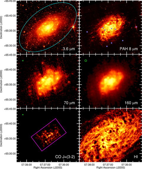
Images of the entire optical disc of NGC 2403 in multiple wave bands. The 3.6 μm image traces starlight. The PAH 8 μm image traces primarily PAH emission. The 70 and 160 μm images trace cold dust emission. The CO J= (3–2) image shows CO emission associated with molecular gas. The H i image shows atomic gas emission. All images are 21 × 18 arcmin² with north up and east to the left. Logarithmic colour scales are used for all images except the 160 μm image, where the logarithmic scale to the second power was used to enhance the structure in the image, and the CO J= (3–2) image, where a linear colour scale was used. The colour scales were selected so as to best enhance the structures visible in the optical disc of the galaxy. Green circles in the upper left corners of the images show the beam size when the FWHM is greater than 10 arcsec; smaller beam sizes are difficult to illustrate in this image. The optical disc of the galaxy, as defined by de Vaucouleurs et al. (1991), is shown as a cyan ellipse in the 3.6 μm image. The blue circles in the PAH 8 μm image show the positions of foreground stars that were brighter than or as bright as the continuum emission from the galaxy at 8 μm. These stars were masked out in the analysis. The magenta box in the CO J= (3–2) image shows the region observed with HARP-B. Pixels with non-detections in the CO data are set to black.

Open in new tabDownload slide

Figure 2

Images of the inner 12 × 9 arcmin² of NGC 2403 in multiple wave bands. The 3.6, 8.0, 70, 160 μm, CO J= (3–2) and H i images are the same as the images in Fig. 1 except that the images are cropped and that the colour scales have been adjusted to show greater contrast in the centre. The colours in the two additional CO J= (1–0) images [from the BIMA SONG survey and from the NRAO 12 m observations by Thornley & Wilson (1995)] are scaled linearly. The magenta box in the CO J= (1–0) image from the NRAO 12 m shows the region that was covered in the observations. Pixels with non-detections in the CO data are set to black. The cyan square indicates the location of VS 44, which is region 44 in the catalogue by Véron & Sauvayre (1965) and region 128 in the catalogue by Hodge & Kennicutt (1983). See the caption for Fig. 1 for additional information on the other symbols and lines in the figure.

Open in new tabDownload slide

The stellar emission, which is shown by the 3.6 μm image, looks similar to what is expected for a late-type spiral galaxy; the bulge is close to non-existent and the disc, while well-defined, has a clumpy structure. The PAH 8 μm image shows the clumpy dust structures in the ISM. Some of these structures are also visible in the 70 and 160 μm images despite the lower resolution of the data. The overall structure of dust emission is fairly typical compared to most late-type spiral galaxies (Bendo et al. 2007). The CO J= (3–2) and J= (1–0) images all appear similar to each other. Some of the structures seen in the CO emission, such as the spiral arm structure to the west of the centre and a few CO-bright regions such as VS 44, are similar to those traced by PAH and longer wavelength dust emission. However, the CO maps contain a notable hole close to the centre of the optical disc, whereas PAH 8 μm and longer wavelength dust emission is still present in this region. Interestingly, this hole corresponds to the peak in diffuse X-ray emission found by Fraternali et al. (2002). We discuss this further in Sections 5 and 6. In contrast to all of these images, the H i emission is much more extended; the emission is detectable well outside the optical disc of the galaxy. A number of shell-like structures are visible within the H i data. These shells were also identified by Thilker, Braun & Walterbos (1998), who associated them with star-forming regions. While bright objects in many of the other wave bands, such as VS 44, do not have H i counterparts, some of the shells in the H i image, such as the ones at α= 7:37:15 δ=+65:34:30 and α= 7:36:50 δ=+65:37:30, do have counterparts in other wave bands.

Figs 3 and 4 show the dust surface density and temperature maps derived as part of the analysis in Section 2.2. The dust mass image exhibits structures that appear similar to those seen at 70 and 160 μm. However, star-forming regions appear notably enhanced in the temperature map. The dust temperatures range from 26 K in infrared-bright regions (including VS 44) to 17 K in the fainter diffuse regions. Note that the <20 K regions located at approximately α= 7:37:20 δ=+65:40:00 and α= 7:36:35 δ=+65:32:00 may have been affected by latent image effects in the 70 μm band. The median temperature is 22 K. These temperatures are similar to those measured in other nearby galaxies when single thermal components have been fitted to far-infrared ISO or Spitzer data that sample the peak of the thermal dust emission from 60 to 200 μm (e.g. Popescu et al. 2002; Bendo et al. 2003; Engelbracht et al. 2004; Regan et al. 2004; Bendo et al. 2006; Perez-Gonzalez et al. 2006).

Figure 3

Image of the dust surface density in NGC 2403 produced after the analysis in Section 2.2. The surface densities were corrected for the inclination of this galaxy [given as by de Blok et al. (2008)]. The image size and orientation are the same as the size and orientation of the images in Fig. 1. The green circle in the upper left corner shows the 38 arcsec FWHM of the PSF, which is equivalent to the PSF of the 160 μm data. The uncertainties in the data are ∼20 per cent. The black square indicates the location of VS 44.

Open in new tabDownload slide

Figure 4

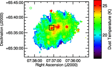
Image of the dust temperatures in NGC 2403 produced after the analysis in Section 2.2. The image size and orientation are the same as the size and orientation of the images in Fig. 1. The green circle in the upper left corner shows the 38 arcsec FWHM of the PSF, which is equivalent to the PSF of the 160 μm data. The uncertainties are ≲1 K. The black square indicates the location of VS 44. Regions with temperatures of <20 K at α= 7:37:20 δ=+65:40:00 and α= 7:36:35 δ=+65:32:00 may have been strongly affected by latent image effects.

Open in new tabDownload slide

4 THE CO J= (3–2)/J= (1–0) RATIO AND THE CONVERSION FROM LINE INTENSITY TO MOLECULAR GAS SURFACE DENSITY

Given the superior resolution of the HARP-B CO J= (3–2) data compared to the older NRAO 12 m CO J= (1–0) data and given the superior spatial coverage of the HARP-B data to both the NRAO 12 m and BIMA SONG data, it would be preferable to use the HARP-B data to calculate molecular gas surface densities for comparisons to dust emission, particularly PAH 8 μm emission. However, the conversion from CO line emission to molecular gas mass (X_CO) is generally based on the CO J= (1–0) line. Therefore, the CO J= (3–2)/J= (1–0) ratio needs to be determined to convert the CO J= (3–2) line to a molecular gas surface density.

For this analysis, we compared the HARP-B CO J= (3–2) data to the NRAO 12 m CO J= (1–0) data from Thornley & Wilson (1995) for the reasons discussed in Section 2.3.2. We examined both median line intensities and intensities measured in the pointing positions used by Thornley & Wilson (1995). For these comparisons, we use intensities based on the main beam temperatures. For comparing median line intensities, we used CO J= (3–2) data where the resolution and pixels are matched to those of the CO J= (1–0) data, and we only selected pixels that are 3σ detections in both images. The median CO J= (1–0) line intensity in these pixels is 1.56 K km s⁻¹, while the median CO J= (3–2) intensity is 1.08 K km s⁻¹. This gives a median CO J= (3–2)/J= (1–0) line ratio of 0.69. The standard deviation of the ratio across the disc is 0.29. Fig. 5 shows how the line ratio varies across the centre of the galaxy. The ratio does not appear to exhibit any clear structure, although the ratio is low in the south-east side of the region, which corresponds to a location where the CO J= (3–2) ratio is also low. The ratios range from 0.11 ± 0.3 to 1.2 ± 0.3.

Figure 5

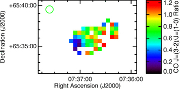
Image of the CO J= (3–2)/J= (1–0) line ratio for the central 12 × 9 arcmin² of NGC 2403. The orientation, size and central coordinates of the image have been selected to match those of Fig. 2. The 30 arcsec pixels correspond to the positions of the pointed observations performed by Thornley & Wilson (1995). To make this plot, the PSF of the data in the CO J= (3–2) data cube was matched to the PSF of the CO J= (1–0) data, the CO J= (3–2) line intensities were measured and then the CO J= (3–2) data were rebinned to match the pixel scale of the CO J= (1–0) data. The green circle in the upper left corner shows the 54 arcsec PSF of the CO J= (1–0) data. The uncertainties in this ratio are mainly dependent on the uncertainties in the CO J= (1–0) data; the typical S/N values range from 3σ to 8σ. Locations where line emission was not measured above the 3σ level and locations affected by artefacts along the edge of the region observed in the CO J= (3–2) line were left blank.

Open in new tabDownload slide

For comparison, Thornley & Wilson (1994) and Wilson, Walker & Thornley (1997) measured ratios for individual giant molecular clouds in M33 ranging from 0.4 to 0.8, and Mauersberger et al. (1999) measured CO J= (3–2)/J= (1–0) ratios in 28 nearby spiral galaxies ranging from 0.2 to 0.7. The median CO J= (3–2)/J= (1–0) ratio for NGC 2403 appears high but typical compared to these other measurements. However, the factor of 10 variation in the CO J= (3–2)/J= (1–0) ratio across the disc of NGC 2403 is high compared to what was measured by these other surveys, and the minimum and maximum fall outside the typical ranges of the objects in the other surveys. It is quite possible that the variations in the ratio that we observed in NGC 2403 are real and that such variations have not been observed in other surveys either because the regions were unresolved or undetected. Wilson et al. (2009) using CO J= (3–2) data from the JCMT NGLS found evidence for CO J= (3–2)/J= (1–0) ratios that vary by a factor of 10 in NGC 4569 as well. It could be possible that further analysis of the JCMT NGLS data will reveal that such variations are actually typical for nearby galaxies.

Given the strong variations in the ratio, we did not feel confident about applying a simple scaling term to the CO J= (3–2) data to scale it to match the CO J= (1–0) data. We therefore examined how the CO J= (3–2)/J= (1–0) ratio could be derived from either the radius or the CO J= (3–2) surface brightness. For this analysis, we used the CO J= (3–2) and J= (1–0) data that were prepared for Fig. 5. A fit between log(CO J= (3–2)/J= (1–0)) and a linear function of both log(CO J= (3–2)/(K km s⁻¹)) and radius [calculated using the inclination of given by de Blok et al. (2008)] resulted in the lowest reduced χ² value. The relation is

8

Fig. 6 shows the relation between the CO J= (3–2)/J= (1–0) intensity ratio and CO J= (3–2) intensity, the relation between the intensity ratio and radius, and the relation given by equation (8). The dependence of the ratio on CO J= (3–2) intensity is very apparent, but the dependence of the ratio on radius is fairly weak. None the less, including a term for radius in the conversion between the CO J= (3–2) intensity and the CO J= (3–2)/J= (1–0) ratio does provide a better fit (in terms of the reduced χ²) than a function that does not include such a term. We also found that Pearson's correlation coefficient increased from 0.54 for the data in the left-hand panel to 0.81 for the data in the right-hand panel of Fig. 6, confirming that the extra radial distance term reduced the scatter. Based on the scatter around the relation given in equation (8), the conversion from the CO J= (3–2) intensity to the CO J= (1–0) intensity should be accurate to within 20 per cent.

Figure 6

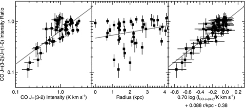
The CO J= (3–2)/J= (1–0) intensity ratio plotted as a function of CO J= (3–2) intensity (left-hand panel), radius (centre panel) and the right-hand side of equation (8) (right-hand panel). The data points are for the 30 arcsec² regions shown in Fig. 5. The grey lines are the best-fitting lines to the data.

Open in new tabDownload slide

Given these results, we can now scale the CO J= (1–0) to H₂ conversion factor for use with the CO J= (3–2) line. X_CO for the J= (1–0) transition may depend on several environmental factors. In particular, it has been shown that it may be dependent on metallicity (e.g. Wilson 1995; Israel 1997b; Israel 2000; Barone et al. 2000; Israel et al. 2003; Strong et al. 2004; Israel 2005). We have decided to use the conversion

9

proposed by Israel (2000), which is based on determining the X_{CO J= (1−0)} needed to keep the ratio of total gas surface density to far-infrared surface brightness constant in CO clouds in the Large and Small Magellanic Clouds. This equation is also found to be in agreement with measurements based on gamma-ray emission from the Milky Way (Strong et al. 2004). We use this equation along with the abundance gradients given in Section 2.6 in one set of calculations of the molecular gas surface densities.

However, recent observational results in which the CO velocity dispersions, radii and CO luminosities of giant molecular clouds are used to infer their mass and hence X_{CO J= (1−0)} suggest that the conversion factor does not vary with metallicity (Blitz et al. 2007; Bolatto et al. 2008), contradicting the results derived using other methods. Therefore, we also use a second set of molecular gas surface density data calculated using X_{CO J= (1)}= 1.9 × 10²⁰ cm⁻² (K km s⁻¹)⁻¹, which was derived by Strong & Mattox (1996) using models of gamma-ray scattering that did not include radial variations.

Israel (1997b) indicated that radiation field strength could be a second factor that affects X_co, although some authors have not found evidence for such a dependency (e.g. Bolatto et al. 2008). The application of the relation found by Israel (1997b) to our data does not appear straightforward. The metric for radiation field intensity used by Israel (1997b) uses the ratio of the far-infrared surface brightnesses measured using IRAS data to the neutral hydrogen density. Because IRAS data do not sample the Rayleigh–Jeans side of the dust SED in the same way that Spitzer data do, we would need to convert the far-infrared fluxes derived from Spitzer data to match those calculated from IRAS data, which may not be straightforward. Moreover, Israel (1997b) derived his relation using subregions within dwarf galaxies where radial variations in abundances were not present and therefore where variations in the gas-to-dust ratio should not be present, whereas NGC 2403 clearly exhibits radial variations in abundances and therefore may exhibit radial variations in the gas-to-dust ratio that would affect the radiation field intensity metric. Fortunately, Israel (1997b) found that it should still be possible to derive a reasonable approximation for X_CO based on its relation to oxygen abundances alone. Therefore, for simplicity, we will not attempt to include an additional correction to X_CO for radiation field intensity, although we still discuss the implications of this dependency when appropriate.

5 COMPARISON OF ATOMIC GAS, MOLECULAR GAS AND DUST SURFACE DENSITIES

To compare the molecular, atomic and dust surface densities, we first measured the radial profiles of the surface densities as well as the gas-to-dust ratios. First, all data were convolved with kernels that match the PSFs to those of the 160 μm data before radial profiles were extracted. The gas-to-dust ratio was calculated on a pixel-by-pixel basis from images regridded to match the astrometry of the dust surface density images. We then measured means, standard deviations and uncertainties in mean values within elliptical annuli with widths along the major axes that were equal to 2 pixels (or 9 arcsec in the dust and gas-to-dust ratio data, 14.6 arcsec in the molecular gas data and 2 arcsec in the atomic gas data). This method for setting the annuli widths was used to avoid problems with noise caused by having too few pixels fall within given annuli, but the resulting annuli are small enough that the data, which have a PSF with an FWHM of 38 arcsec, will be Nyquist-sampled. Pixels where CO or H i line emission was not detected were set to 0 in those data. The ratio of the axes in the elliptical annuli was set to account for the inclination of the galaxy (⁠⁠; de Blok et al. 2008).

Fig. 7 shows the radial profiles of the H i, H₂ and dust surface densities. Two versions of the H₂ surface densities are shown. The values shown with a solid line were calculated using a constant X_CO and the values shown with the dotted line were calculated using the formula for X_CO given in equation (9). For simplicity, we will refer to the former as the constant X_CO molecular gas surface density and the latter as the variable X_CO molecular gas surface density. Although the standard deviation in the CO J= (3–2) radial profiles approaches the same level as the mean values at large radii, the uncertainties in the mean values are no wider than the thicknesses of these lines. Hence, the mean values are very well defined even though significant variance may be seen in CO intensities at specific radii.

Figure 7

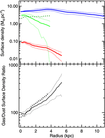
Radial profiles of the H i surface density (solid blue line, top panel), H₂ surface density (green lines, top panel) and dust surface density (solid red line, top panel) as well as the total (molecular and atomic) gas-to-dust surface density ratio (bottom panel) plotted up to 10 kpc, which is equivalent to the edge of the optical disc. For the H₂ and gas/dust ratios, the solid lines are for quantities calculated using a constant X_CO and the dotted lines are for quantities calculated using a value of X_CO that depends on 12+log(O/H). The standard deviations of the data are plotted as thinner lines around all radial profiles except for the H₂ surface density and gas-to-dust ratios calculated with a variable X_CO, which have standard deviations that are similar to the equivalent quantities calculated with the constant X_CO. The uncertainties in the mean values are generally smaller than the thicknesses of these lines. The H₂ and dust radial profiles are truncated at the maximum radii where the quantities could be reliably measured along the major axis (4 and 5.5 kpc, respectively). The gas-to-dust ratio calculated using the constant X_CO is also truncated at the maximum radius at which the dust surface densities could be measured. The gas-to-dust ratio calculated using the variable X_CO is truncated at 4 kpc to show how the change in X_CO affects this ratio; beyond this radius, the radial profile merges back into the other gas-to-dust radial profile.

Open in new tabDownload slide

The figure shows that most of the mass in the ISM of this galaxy is traced by the H i emission, a result also obtained by Thornley & Wilson (1995). The H i surface density is relatively flat; it increases slightly towards 4 kpc and then declines gradually beyond that radius. The constant X_CO molecular gas surface density decreases exponentially with radius. The scale length of the constant X_CO molecular gas radial profile is 2.32 ± 0.07 kpc. The variable X_CO molecular gas surface density, however, is so close to flat that it is not possible to accurately fit an exponential function to the profile. The dust surface density, like the constant X_CO molecular gas surface density, decreases with radius. Its radial profile has an exponential scale length of 3.16 ± 0.10 kpc. If we applied an additional correction for radiation field strength in X_CO, then this would increase the molecular gas surface density in regions with high radiation field intensities, which would correspond to regions in the centre of NGC 2403 with higher dust temperatures shown in Fig. 4. Therefore, the molecular gas surface density radial profile would fall in between those of the constant X_CO and variable X_CO molecular gas surface densities plotted in Fig. 7.

Of particular interest is how the radial profiles of the molecular gas change when the abundance-dependent correction is introduced. If the variable X_CO molecular gas surface density is an accurate depiction of the true surface density, then it implies that ∼25 per cent of the ISM at large radii is comprised of molecular gas. If true, this would contradict the typical depiction of how the ratio of molecular to atomic gas varies within spiral galaxies, with the centres of galaxies being dominated by molecular gas and the outer discs being dominated by atomic gas (e.g. Wong & Blitz 2002; Bigiel et al. 2008). However, these prior results rely upon the assumption that X_CO is constant. This issue should be examined further using radial profile data for other galaxies and using deeper CO data to determine if molecular gas surface densities calculated using an X_CO that depends on metallicity are found to still be significant contributors to the total gas surface density at larger radii and in other galaxies. If found to be true, then we need to more carefully consider how to convert CO intensities into molecular gas surface densities and possibly revise the standard depiction of the structure of the ISM in spiral galaxies.

The bottom panel of Fig. 7 shows two radial profiles of the gas-to-dust ratio based on the two different molecular gas surface densities used in this analysis. Both radial profiles increase relatively smoothly with radius. Because the atomic gas is the largest component of the ISM, differing assumptions in X_CO have only a minor impact on the radial profiles within the range shown. Within a kpc of the centre, the ratio is seen to drop to ∼100. For comparison, the expected gas-to-dust ratio in the Milky Way near the Earth, based either on the measurement of the depletion of metals from the gaseous phase of the ISM or on the ratio of gas column densities to optical extinction, is 100–200 (Krügel 2003; Whittet 2003; Li 2004; Krügel 2008). As we indicated above, the dust masses that we have calculated are low compared to more sophisticated models of dust emission, so it is unlikely that we have underestimated the central gas-to-dust ratio. Instead, it is quite possible that the ISM in the centre of NGC 2403 is relatively dust-rich. The gas-to-dust ratio reaches a value of ∼150 at about 2 kpc. At radii of 5.5 kpc, which is the limit of where we can accurately measure the radial profile of the dust in this galaxy, the ratio reaches ∼400.

Fig. 8 shows the total gas-to-dust ratio for all pixels in which we measured dust masses. To make this image, the data were convolved with kernels that match the PSFs to those of the 160 μm data (which has an FWHM of 38 arcsec). This image shows that the gas-to-dust ratio appears to increase monotonically with radius. Most of the structures visible in Figs 1 and 3 are not at all visible. Even VS 44, which has a very high surface brightness in many of the images shown in Fig. 2, appears indistinct in Fig. 8 compared to other locations at similar radii. The only features that are not radially symmetric are the streaks at the north-west and south-east edges of the mapped data that are a result of the latent image artefacts in the 70 μm data. The results from Fig. 8 suggest that the gas-to-dust ratio is primarily dependent on radius and that it does not vary significantly between diffuse and star-forming regions.

Figure 8

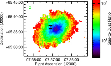
Image of the gas-to-dust surface density ratio in NGC 2403. The image is 21 × 18 arcmin² with north up and east to the left. Only pixels where the dust mass was measured are shown. The molecular gas surface densities were calculated assuming that X_CO is constant, although the functionality of X_CO does not strongly affect the appearance of this figure. The green circle in the upper left corner shows the 38 arcsec FWHM of the PSF, which is equivalent to the PSF of the 160 μm data. The black square indicates the location of VS 44.

Open in new tabDownload slide

Fig. 8 is only useful as a qualitative demonstration of how the gas-to-dust ratio depends primarily on radius and not on gas surface density. As an additional quantitative demonstration of this phenomenon, we used techniques similar to what were used by Bendo et al. (2008) in their comparisons of PAH 8, 24 and 160 μm emission. We used the H i, H₂ (calculated using a constant X_CO) and dust surface density maps that were used to create Fig. 8. We rebinned these data into 45 arcsec pixels. This pixel size was selected because it is an integer multiple of the pixel size used for the MIPS data that is also close to the 38 arcsec FWHM of the 160 μm data. We then extracted the surface densities from each 45 arcsec² region in the data. Because the H i is the dominant component of the ISM in this galaxy, the choice of X_CO in this analysis has a minor impact on the results.

Fig. 9 shows that the total gas density is related to the total dust density for these 45 arcsec² regions, but the relation exhibits significant scatter. For a given gas surface density, the dust surface density could vary by a factor of 5. Fig. 10 shows how the gas-to-dust ratio varies with gas surface density. This is an alternative form for plotting the data in Fig. 9; if a one-to-one relation existed between the gas and dust surface densities, then the relation in Fig. 10 should have a slope of 0 and exhibit little scatter. The data in Fig. 10 actually exhibit a negative slope [−79 ± 13 (M_⊙ pc⁻²)⁻¹] and significant scatter. Fig. 11 shows how the gas-to-dust ratio varies with the galactocentric radius for these 45 arcsec² regions. The relation here shows much less scatter; gas-to-dust ratios at a given radius may vary by a factor of 2 or less.

Figure 9

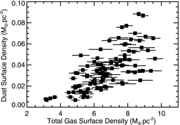
The dust surface density versus the total (atomic and molecular) gas surface density for 45 arcsec² regions in NGC 2403. The data were extracted from images that had all been convolved with kernels that match the PSFs to those of the 160 μm data. Only regions within 5.5 kpc (the limit at which the dust masses can be reliably measured) and with S/N of >5 were used. Uncertainties in the ordinate are generally smaller than the symbols in this plot and the next two plots. See the text in Section 5 for a description of how these surface densities were extracted.

Open in new tabDownload slide

Figure 10

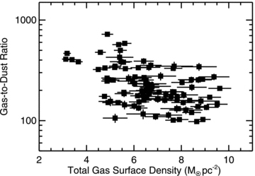
The gas-to-dust ratio versus the total (atomic and molecular) surface density for 45 arcsec² regions in NGC 2403. See the caption for Fig. 9 for additional information.

Open in new tabDownload slide

Figure 11

The gas-to-dust ratio versus radius for 45 arcsec² regions in NGC 2403. This can be considered an alternate version of the bottom panel in Fig. 7. See the caption for Fig. 9 for additional information.

Open in new tabDownload slide

Using Spearman's rank correlation coefficient, which is a non-parametric correlation coefficient that is useful when dealing with data that may exhibit non-linear (i.e. exponential) relations, we can demonstrate that the relation in Fig. 11 is more significant than the relation in Fig. 9. For reference, perfectly correlated data would have a coefficient of 1 and uncorrelated data would have a coefficient of 0. The correlation coefficient for the relation between gas and dust surface densities in Fig. 9 is 0.73, which would imply a good correlation. However, the correlation coefficient for the relation between the gas-to-dust ratio and radius is 0.91. These results demonstrate that the relation between the gas-to-dust ratio and radius places stronger constraints on dust surface densities than the total gas surface density by itself. Moreover, this quantitative approach confirms that the absence of visible structure in Fig. 8 is not simply a consequence of the poor resolution of the data. Instead, it is a result of the gas-to-dust ratio being primarily dependent on radius. However, it is always possible that local variations in the gas-to-dust ratio will be visible in higher resolution data.

The most obvious driver for this gradient in the gas-to-dust ratio is the decrease in metallicity with radius that has been observed previously (see Section 2.6). The gas-to-dust ratio is naturally expected to increase as abundances decrease simply because fewer constituents of dust should be present in the ISM. Gas-to-dust ratios significantly higher than the local Milky Way value of ∼150 have been measured in many dwarf galaxies with low metallicities (e.g. Lisenfeld & Ferrara 1998; Walter et al. 2007), and globally integrated measurements of gas-to-dust ratios are correlated with globally integrated 12+log(O/H) or metallicity measurements (e.g. Issa, MacLaren & Wolfendale 1990; James et al. 2002; Draine et al. 2007; Hirashita et al. 2008). Moreover, Lisenfeld & Ferrara (1998) and Mũnoz-Mateos et al. (2009) have found linear relations between oxygen abundances and dust-to-gas ratios in nearby galaxies. Although the dust-to-gas ratios typically decrease faster than the oxygen abundances in these relations, the slopes are still on the order of 1.

As stated in Section 2.6, the typical gradient in 12+log(O/H) that has been measured in NGC 2403 is −0.084 ± 0.009 dex kpc⁻¹. For comparison, we measured the gradient in the logarithm of the dust-to-gas ratio [d log(σ_dust/σ_gas)/dr] to be −0.097 ± 0.002 dex kpc⁻¹ for NGC 2403. These gradients are so close that it implies that the dust-to-gas ratio is primarily dependent on metallicity. Alternatively, when we calculated 12+log(O/H) as a function of radius, we found that the relation between 12+log(O/H) and d log(σ_dust/σ_gas)/dr had a slope of 0.86 ± 0.02. This slope is less than 1, which is consistent with the results obtained by Lisenfeld & Ferrara (1998) and Mũnoz-Mateos et al. (2009), but it is so close to 1 that it implies a linear relationship between the oxygen abundance and the dust-to-gas ratio. Variations in the ratio of oxygen to the other constituents of dust could explain the difference in the gradients. Garnett et al. (1999), for example, have shown that C/O increases systematically with O/H within this galaxy as well as within M 101, and since carbon is a primary constituent of dust, d log(σ_dust/σ_gas)/dr would be expected to be steeper than the gradient in 12+log(O/H). Additional comparisons between radially averaged dust-to-gas ratios and 12+log(O/H) using all of the data from SINGS, THINGS and the JCMT NGLS would be appropriate for determining whether similar results are typically obtained for all spiral galaxies.

Some researchers (e.g. Neininger et al. 1996; Israel 1997a) have suggested that X_CO for any galaxy can be determined in a two-step process. First, the gas-to-dust ratio is measured in a region dominated by atomic gas. Secondly, this ratio is applied to a region that contains CO and dust emission to determine how much molecular gas should be present, thus giving X_CO. However, the results here show that the application of this method to spiral galaxies must be performed cautiously. The first problem is that this method assumes that the gas-to-dust ratio is constant, whereas we have demonstrated that it varies with radius. The second problem is that, as explained in Section 4, X_CO may depend on metallicity, and metallicity will vary with radius in most nearby galaxies. Despite these problems, it may still be possible to derive X_CO within subsections of galaxies by dividing the galaxies into elliptical annuli where both the metallicity and the gas-to-dust ratio will remain constant. If regions free of molecular gas but containing detectable atomic gas and dust emission can be identified within the individual annuli, then these locations can be used to measure the gas-to-dust ratio at specific radii. These regions can then be used to infer the gas-to-dust ratio for locations at similar radii that contain detectable CO emission to determine how much gas should be present and therefore what X_CO is needed to account for all of the gas. This will then lead to a measure of X_CO as a function of radius. Unfortunately, it is not possible to apply this method to the data used here. To perform this analysis correctly, we would need to work with data where the PSFs match the 40 arcsec resolution of the 160 μm data. When the CO data are matched to the 160 μm PSF, the area within radii of 4 kpc [the region in which CO J= (3–2) emission is detected along the major axis] contains almost no CO-free regions for comparison to regions where CO is detected.

It is possible that the observations here may have missed the presence of very cold dust (dust with temperatures of <15 K that may not contribute strongly to the 70 and 160 μm bands but that may constitute the bulk of the dust mass at larger radii. As argued in Appendix A, it is unclear in cases where submillimetre emission has been observed in excess of the ∼20 K thermal dust models fit to the 70 and 160 μm data whether this excess originates from large masses of <15 K dust or very low masses of dust with enhanced submillimetre emissivities. Results from previous analyses have suggested that estimates of the dust mass based on the 70 and 160 μm wave bands should be well within an order of magnitude of the expected dust mass (Lisenfeld et al. 2002; Dumke, Krause & Wielebinski 2004; Regan et al. 2004; Bendo et al. 2006; Draine et al. 2007). Based on these previous results, we expect the gas-to-dust ratio shown in Fig. 7 to be accurate and to not be strongly affected by large masses of dust not traced by the 70 and 160 μm bands. It is none the less possible that the radial increase in our measured gas-to-dust ratio could be linked to an increase in the relative fraction of <15 K dust with radius, but to properly determine this will require both submillimetre measurements of the dust emission and models of this dust emission that incorporate accurate submillimetre emissivities based on laboratory and theoretical results.

6 COMPARISON OF PAH, CO J= (3–2) AND H i EMISSION

As we are interested in re-examining the empirical correlation between CO and PAH emission found by Regan et al. (2006) using the higher sensitivity HARP-B data, and as they used radial profiles to show this correlation, we will first look at the radial profiles for the CO J= (3–2) intensity and PAH 8 μm surface brightness. Since Regan et al. (2006) used the CO intensities for their analysis instead of converting the CO intensities to molecular gas surface densities, we will compare the PAH 8 μm surface brightnesses directly to the CO J= (3–2) intensities.

The radial profiles for the H i intensity, CO J= (3–2) intensity and PAH 8 μm surface brightness are shown in Fig. 12. All data were convolved with kernels that match the PSFs to those of the CO J= (3–2) data (which has an FWHM of 14.5 arcsec) before radial profiles were extracted. The techniques used for extracting these radial profiles are the same as those used in Section 5, although we only used data in which the CO emission was detected to calculate the CO J= (3–2)/PAH 8 μm ratio. The width of the elliptical annuli along the major axis in the CO J= (3–2) and CO J= (3–2)/PAH 8 μm ratio that we used was equivalent to 2 pixels (or 14.6 arcsec), which does not result in Nyquist-sampled radial profiles. However, using narrower elliptical profiles results in excessive noise because of the low numbers of pixels falling within the elliptical annuli. While the standard deviations in the CO J= (3–2) and PAH 8 μm radial profiles are sometimes greater than the plotted radial means, just as was the case with the CO radial profiles in Fig. 7, the standard deviation does not equate to the uncertainties in the means. The uncertainties in the means are actually smaller than the thickness of the lines in Fig. 12 except for the ratio of the CO J= (3–2) intensity to PAH 8 μm surface brightness. In effect, we can actually measure the means to a relatively high precision, but we still see significant variance in the data.

Figure 12

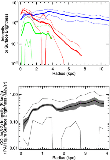
Radial profiles of the H i intensity in Jy beam⁻¹ km s⁻¹ (blue line, top panel), CO J= (3–2) intensity in K km s⁻¹ (green line, top panel) and PAH 8 μm surface brightness in MJy sr⁻¹ (red line, top panel) as well as the ratio of CO J= (3–2) intensity to PAH 8 μm surface brightness (black line, bottom panel) plotted up to 10 kpc, which is equivalent to the edge of the optical disc. All data were convolved with kernels that match the PSF of the CO J= (3–2) data (which has an FWHM of 14.5 arcsec) before radial profiles were extracted. The standard deviations of the data are plotted as thinner lines around all radial profiles. The uncertainties in the mean values are generally smaller than the thicknesses of these lines except in the case of the CO J= (3–2)/PAH 8 μm emission ratio, where the uncertainty is shown as a shaded grey region. The CO J= (3–2) and PAH 8 μm radial profiles are truncated at the radii beyond which the quantities could be reliably measured on the major axis. The ratio in the bottom panel is also truncated at the maximum radius where CO J= (3–2) intensities could be reliably measured.

Open in new tabDownload slide

In the top panel of the figure, we can see that the radial profiles of the CO J= (3–2) and PAH 8 μm emission are similar to each other. In contrast, the H i radial profile is much broader than either the CO J= (3–2) or PAH 8 μm radial profiles. Given the dissimilarity between the PAH 8 μm and H i radial profiles as well as the dramatic differences between the appearance of the 8 μm and H i images in Figs 1 and 2, we can conclude that the PAH 8 μm emission is not associated with H i in this galaxy. We will not discuss the H i further but instead focus on the comparison between the CO J= (3–2) and PAH 8 μm.

The CO J= (3–2) and PAH 8 μm radial profiles not only appear superficially similar but also have similar exponential scale lengths. Between 0.5 and 4 kpc, the CO J= (3–2) radial profile has an exponential scale length of 2.0 ± 0.2 kpc. The PAH 8 μm emission (in the convolved data) has a scale length of 1.99 ± 0.04 kpc over the same range. The plot of the ratio of the two in the bottom panel of Fig. 12 shows that the ratio of 0.5 to 4 kpc has a gradient of 0.070 ± 0.017 (K km s⁻¹) (MJy sr⁻¹)⁻¹ kpc⁻¹, but the mean value for the ratio stays between ∼0.25 and ∼0.6 at radii between 0.5 and 4 kpc. However, while the mean in the CO J= (3–2)/PAH 8 μm ratio remains relatively constant over this range of radii, the high standard deviation shows that the ratio fluctuates greatly at any given radius. The implications of this are discussed further below.

The CO J= (3–2)/PAH 8 μm emission ratio decreases sharply in the nucleus of the galaxy. This drop in the ratio corresponds to drops in the surface brightness in both wave bands. The drop in the ratio may be in part related to variations in the gas-to-dust ratio described in Section 5, but that would not explain why the ratio appears close to constant at larger radii nor would it explain why the CO and PAH emission also drops near the nucleus. We can exclude the possibility that currently ongoing intense nuclear star formation may be inhibiting PAH emission (either through destroying PAHs or through changing their ionization state) and ionizing gas in the centre of the galaxy; both Hα (e.g. Drissen et al. 1999) and 24 μm images (e.g. Bendo et al. 2008) show that the nucleus is relatively quiescent compared to other star-forming regions which do have PAH 8 μm and CO J= (3–2) counterparts. Because this galaxy is classified as having an H ii nucleus (e.g. Ho, Filippenko & Sargent 1997), and no other study indicates the presence of an active galactic nucleus (AGN) in NGC 2403, we can also exclude the possibility that an AGN could be responsible for the decrease in PAH and CO J= (3–2) emission in the nucleus.

The reason for the decrease in PAH 8 μm and CO J= (3–2) in the nucleus of the galaxy may be explained by the simple fact that, like many other late-type spiral galaxies, the ISM is clumpy and that this galaxy does not contain centrally concentrated gas and dust emission (e.g. Bendo et al. 2007). The clumpiness of the ISM would also explain why the standard deviations in the PAH 8 μm and CO J= (3–2) radial profiles in the top panel of Fig. 12 are very large. The CO J= (3–2)/PAH 8 μm emission ratio may decrease towards the centre simply because the two wave bands may not be correlated on sub-kpc scales. The comparison of the PAH 8 μm and CO J= (3–2) images in Section 3 visually demonstrates this; some structures in the PAH 8 μm image were not as bright as those in the CO J= (3–2) image and vice versa. Additionally, the high standard deviation in the radial profile of the CO J= (3–2)/PAH 8 μm ratio implies that the PAH 8 μm and CO emission are not well correlated at any given radius.

For an explicit quantitative analysis to demonstrate that PAH 8 μm and CO J= (3–2) emission does not trace the same structures on small spatial scales, we could not use the same binning procedure used to compare the dust surface density versus total gas surface density in Section 5. The gaps between detected structures in the CO J= (3–2) images made the binned data difficult to interpret. As an alternative, we used surface brightnesses measured in a series of discrete regions. We selected 25 regions with the highest intensity in the CO J= (3–2) image and the 25 regions with the highest surface brightnesses in the PAH 8 μm image [convolved with a kernel to match its PSF to the PSF of the CO J= (3–2) data]. These regions were defined using the coordinate system of the CO J= (3–2) data; each region is 3 × 3 pixel² in the CO J= (3–2) data (21.8 × 21.8 arcsec² or 330 × 330 pc²). Some of the regions overlap, and some regions are not centred on peak-like emission but instead selected to attempt to cover resolved structures. The regions were also selected to avoid locations that may have been severely affected by foreground stars. Any locations that were affected by foreground stars in the PAH 8 μm data were blanked out in both data sets before surface brightnesses were extracted. These regions are shown in Fig. 13. The extracted surface brightnesses are plotted in Fig. 14.

Figure 13

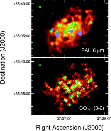
Images of the PAH 8 μm and CO J= (3–2) emission for the central 12 × 9 arcmin² region in NGC 2403 with green squares overlaid to show where intensities or surface brightnesses were measured. The regions selected by their CO J= (3–2) intensities are shown in the CO J= (3–2) image and the regions selected by their PAH 8 μm surface brightnesses are shown in the PAH 8 μm image. See the text for details on the region selection. The PAH 8 μm image has been convolved with a kernel to match its PSF to that of the CO J= (3–2) image. The green circles in the upper left corner of each image show the 14.5 arcsec FWHM of the CO J= (3–2) PSF. Blue regions in the PAH 8 μm image show regions strongly affected by stars that were excluded from the analysis in both wave bands.

Open in new tabDownload slide

Figure 14

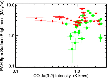
Comparison of the CO J= (3–2) intensity and PAH 8 μm surface brightness for the regions shown in Fig. 13. The regions selected by their CO J= (3–2) intensity are shown as green squares. The regions selected by their PAH 8 μm surface brightness are shown as red triangles.

Open in new tabDownload slide

The relation between CO J= (3–2) and PAH 8 μm surface brightness differs between the two sets of data, demonstrating the presence of regions bright in one band but not in the other. The regions selected in the PAH 8 μm data exhibit virtually no correlation; the Pearson's correlation coefficient for these data is 0.07. The regions selected in the CO J= (3–2) data do exhibit a weak correlation; the data have a Pearson correlation coefficient of 0.32. Given that the square of Pearson's correlation coefficient indicates the fraction of variation in one variable that can be accounted for by a best-fitting line between the data, we find that, in the CO-selected data, only ∼10 per cent of the variation observed in one band can be accounted for by a relation with the other band. In the PAH 8 μm-selected data, <1 per cent of the variation in one band can be accounted for by a relation with the other band. We therefore conclude that, at best, PAH 8 μm emission is only weakly correlated with CO J= (3–2) emission on scales of 330 pc within this galaxy, even though the radial profiles have very similar scale lengths.

We can reject a couple of possible scenarios that would explain why the radial profiles for the PAH μm and CO J= (3–2) emission should match even while the emission mechanisms are not correlated on smaller spatial scales. First of all, PAHs and CO do not share a common origin. PAHs are thought to form in the atmospheres of or outflows from AGB stars or in interstellar shocks (Tielens 2008), while molecular gas is commonly assumed to form on the surfaces of interstellar dust grains (Krügel 2003, 2008). It is also unlikely that the radial profiles are matched through the Schmidt law, which relates star formation to gas surface density (Schmidt 1959; Kennicutt 1998). While star formation is strongly dependent on molecular gas surface densities in subregions within galaxies (Kennicutt et al. 2007; Bigiel et al. 2008; Wilson et al. 2009), PAH emission is not strongly linked to other star formation tracers on sub-kpc scales (e.g. Calzetti et al. 2005, 2007; Thilker et al. 2007; Bendo et al. 2008). Moreover, Bendo et al. (2008) demonstrated that the ratio of PAH 8 μm emission to 24 μm emission (which has been shown to be correlated with other star formation tracers) decreases as a function of radius within NGC 2403, and the ratio of PAH 8 μm emission to other star formation tracers would be expected to vary similarly.

PAH and CO emission could be linked if molecular cloud formation is triggered in regions with stellar potential wells as suggested by Leroy et al. (2008). The new molecular clouds would produce CO emission. Additionally, the increased starlight in these potential wells (from both the stars originally present in the wells and new stars formed from the molecular clouds) would heat the diffuse ISM. According to the results from Bendo et al. (2008), enhanced PAH emission will be produced by locations where the interstellar radiation field has increased. Therefore, the stellar potential wells that form molecular gas clouds in this scenario would not only enhance CO emission but also enhance PAH emission, thus linking the two on large spatial scales and resulting in radial profiles that appear similar for both wave bands. However, the enhanced PAH emission does not need to occur within the stellar potential wells but could instead occur in regions surrounding the potential wells. Therefore, regions containing molecular gas could exhibit CO emission correlated with PAH emission while regions without molecular gas would exhibit PAH emission that is uncorrelated with CO emission as shown in Fig. 14.

It is also possible that both PAH and CO emission are affected by similar excitation mechanisms. As stated by the references cited above, enhancements in PAH emission may be indicative of increased heating of the diffuse ISM, which could be caused by enhancing star formation activity (although they still declared that PAH emission was not useful for tracing star formation on sub-kpc scales). Similarly, Knapen & Beckman (1996) postulated based on the comparison of CO radial profiles to other star formation tracers that CO could be excited by the cosmic rays from star formation, and cosmic rays tend to diffuse into the ISM as can be seen by the comparisons of infrared and radio continuum emission performed by Murphy et al. (2006a,b, 2008). Therefore, increases in star formation could enhance both PAH and CO emission on large spatial scales, which would explain why the radial profiles for PAH and CO emission appear to match each other.

It is also possible that the radial profiles of CO J= (3–2) and PAH 8 μm emission are similar simply by coincidence. The radial profiles of both normalized by the total gas surface density are expected to decrease with radius, although for different reasons. Perhaps the multiplicative factors that relate the slope of the CO J= (3–2) radial profile to that of total gas surface density just happen to match those factors that relate the PAH 8 μm radial profile to that for total gas surface density, at least in this galaxy and the ones studied by Regan et al. (2006). A more extensive investigation using the whole of the JCMT NGLS sample could potentially reveal galaxies where the PAH 8 μm and CO J= (3–2) radial profiles are not similar (i.e. where the radial profiles do not have similar exponential scale lengths). If a sufficient number of such galaxies can be identified, then it would indicate that what was found here was merely a coincidence.

7 CONCLUSIONS

We find that the dust surface density depends on the total (atomic and molecular) gas surface density and on radius. The gas-to-dust ratio varies from ∼100 in the nucleus to ∼400 at 5.5 kpc, which is the limit at which the dust surface densities can be detected. The logarithm of the slope for the gas-to-dust ratio [d log(σ_dust/σ_gas)/dr)], which is 0.097 ± 0.002 dex kpc⁻¹, is very close to the slope in 12+log(O/H), which is usually reported as between −0.07 and −0.09 dex kpc⁻¹. This implies that the gas-to-dust ratio is strongly dependent on metallicity. Additional abundance variations, such as variations in the C/O ratio, could explain the small disparity between d log(σ_dust/σ_gas)/dr and 12+log(O/H). Aside from these strong radial variations in the gas-to-dust ratio, the ratio does not appear to vary within the galaxy.

We also find that the PAH 8 μm and CO J= (3–2) radial profiles have statistically identical scale lengths. On spatial scales of 330 pc, however, PAH 8 μm and CO J= (3–2) emission are uncorrelated. We propose two mechanisms that could link the PAH emission with star formation. First, the CO emission may appear associated with PAH emission if molecular cloud formation is triggered by stellar potential wells. The stars in these potential wells would enhance the radiation field that heats the diffuse ISM, which would enhance PAH emission. Thus, the PAH emission would appear associated with CO emission on large scales but not on small scales. Secondly, the two wave bands may be related through different excitation mechanisms that are linked through star formation and that affect the ISM on large areas. While PAH emission does not trace star formation on sub-kpc scales, it is expected to be enhanced by increases in the interstellar radiation field that accompany enhanced star formation. Meanwhile, CO emission could be enhanced by the increase in cosmic rays that accompanies enhanced star formation. Thus, radially averaged PAH and CO emission would both be linked through star formation, even though PAH and CO emission may not be spatially correlated on sub-kpc scales. However, we also do not rule out the possibility that the PAH and CO emission may just coincidentally have radial profiles with similar scale lengths.

This paper is only a first look at the gas-to-dust ratio and the relation between PAH and CO emission within the JCMT NGLS sample. The SINGS, THINGS and JCMT NGLS samples were all selected to contain many of the same galaxies. The subset of galaxies found in all three samples can be used for an extended comparison of dust, molecular gas and atomic gas surface densities and for comparisons of PAH to CO emission. Moreover, the gradients in the gas-to-dust ratio could then be compared to abundance gradients to examine the relation between the two further.

We thank the reviewer for his/her comments on this paper. The JCMT is operated by The Joint Astronomy Centre on behalf of the Science and Technology Facilities Council of the United Kingdom, the Netherlands Organisation for Scientific Research and the National Research Council of Canada. GJB and DLC were funded by STFC. The research of JI and CDW is supported by grants from NSERC (Canada). AU has been supported through a Post-Doctoral Research Assistantship from the UK Science & Technology Facilities Council. Travel support for BEW and TW was supplied by the National Research Council (Canada). This research has made use of the NASA/IPAC Extragalactic Database (NED) which is operated by the Jet Propulsion Laboratory, California Institute of Technology, under contract with the National Aeronautics and Space Administration.

REFERENCES

Appendix

APPENDIX A: DISCUSSION ON DUST NOT TRACED BY THE MIPS DATA

It is entirely possible that the 70 and 160 μm bands may have missed significant masses of very cold dust (dust with temperatures of <15 K) within this galaxy. However, it is unclear whether such dust is present.

Many surveys working with Spitzer and submillimetre data have not found evidence for very cold dust. The best examples are the results from Dale et al. (2005) and Draine et al. (2007), who worked with Spitzer and submillimetre data for 17 spiral and S0 galaxies in the SINGS sample and found no submillimetre emission in excess of what was predicted by dust models that did not include <15 K dust. Unfortunately, the quality of the submillimetre data used in these studies was quite variable, so it may not have been feasible for Dale et al. (2005) and Draine et al. (2007) to detect submillimetre emission in excess of what is expected from >15 K dust within most galaxies. A few groups using very high signal-to-noise ratio submillimetre data with ISO or Spitzer data have conclusively demonstrated the presence of emission at wavelengths of >850 μm in excess of what is expected from ∼20 K dust within the Milky Way Galaxy (Reach et al. 1995; Finkbeiner, Davis & Schlegel 1999), NGC 4631 (Dumke et al. 2004; Bendo et al. 2006), NGC 3310 (Zhu et al. 2009) and a few nearby dwarf galaxies (Lisenfeld et al. 2002; Galliano et al. 2003, 2005). Although this could represent emission from a high mass of dust at 5–10 K, most authors have rejected this explanation because it leads to implausibly low gas-to-dust ratios, at least when assuming that the dust would have emissivities that follow a λ⁻² power law and that have values similar to those given by Li & Draine (2001). Galliano et al. (2003, 2005) support the scenario in which 5–10 K dust produces the excess submillimetre emission, but they argue that the dust emissivities would need to follow a λ⁻¹ emissivity function and have emissivity values higher than the Li & Draine (2001) values to avoid problems with infeasibly high dust masses. Other authors have suggested that the observed submillimetre excess emission could be produced by >15 K dust with emissivities that are enhanced above a λ⁻² power law at submillimetre wavelengths. Such dust would include grains with exotic shapes, such as fractal dust grains, which would have relatively high submillimetre emissivities relative to their absorption cross-sections (Reach et al. 1995; Dumke et al. 2004; Bendo et al. 2006), dust in which resonances from impurities in the dust grains enhance the submillimetre emissivity (Reach et al. 1995; Bendo et al. 2006) or grains with shallow dust emissivities (κ_ν∝λ^−β, with β < 2) that would only be visible at submillimetre wavelengths (Finkbeiner et al. 1999; Lisenfeld et al. 2002; Zhu et al. 2009). Additionally, laboratory studies (Agladze et al. 1996; Mennella et al. 1998; Boudet et al. 2005) and at least one theoretical study (Meny et al. 2007) have shown that dust grains exhibit a broad range of emissivities at these wavelengths and that submillimetre dust emissivities can be strongly enhanced above the λ⁻² emissivity function that is commonly used in astronomical research. In all of these alternate scenarios, the mass of the dust that produces the excess submillimetre emission is relatively low, and most of the dust mass should be traced by dust that dominates the SED at <450 μm. Moreover, the results from Lisenfeld et al. (2002), Dumke et al. (2004), Regan et al. (2004), Bendo et al. (2006) and Draine et al. (2007) have demonstrated that, based on the total gas content and expected gas-to-dust ratios for nearby galaxies, most of the dust mass in nearby galaxies can be accounted for by ≳15 K dust emitting at ≥450 μm.

It is always possible that newer >160 μm data from either the Herschel Space Observatory or SCUBA2 on the JCMT along with improved dust models could demonstrate that the use of Spitzer data alone will lead to significant underestimates of dust masses. However, based on current data and models, the dust masses that we measure using only the Spitzer data should provide a reasonably accurate estimate of the dust masses. We should not be severely underestimating the dust masses because we have not accounted for large masses of cold dust emitting >160 μm.