Relativistic hybrid stars with super-strong toroidal magnetic fields: an evolutionary track with QCD phase transition Free

Abstract

1 INTRODUCTION

A very hot topic in hadronic and nuclear physics is to search the phase transition from baryons to their constitutes – deconfined quarks. Heavy-ion colliders such as RHIC (Brookhaven) and LHC (CERN) are now in line in order to explore the quantum chromodynamics (QCD) phase diagram for the high temperature and small baryon density regimes, for which lattice QCD calculations predict a smooth cross-over to the QCD phase transition (see Stephanov 2004 for review).

Conversely for the low temperature and high baryon density regimes, compact stars are expected to provide a unique window on the phase transition at their extreme density with a super-strong magnetic field. It has been suggested a long time back that quark matter may exist in the interior of compact objects (Itoh 1970; Bodmer 1971; Witten 1984). Hybrid stars (and strange quark stars) are considered to be such objects, which feature quark cores surrounded by a hadronic matter mantle (or quark cores only; for reviews, see e.g. Weber 1999; Glendenning 2001). Even if the relevant conditions could be reached in a laboratory in the near future (Senger 2004), the conditions prevailing in the compact stars will be different from those produced in accelerators, i.e. the matter will be long-lived, charge neutral and in β-equilibrium with respect to weak interactions. It is therefore important to investigate the properties of such ‘exotic’ stars, providing hints about the main features of matter at those extreme conditions.

The formation of the quark cores in compact stars is expected to take place by a first-order phase transition (Glendenning 1992, 2001). Albeit still very uncertain (e.g. Horvath 2007), such a transition would proceed by the conversion of initially metastable hadronic matter in the core into the new deconfined quark phase. The metastable phase could be formed as the central density of neutron stars exceeds a critical value, due to mass accretion, spin-down or cooling. Possible astrophysical sites are present in protoneutron stars during the collapse of supernova cores [near the epoch of bounce (Takahara & Sato 1985; Yasutake et al. 2007) or at the late post-bounce phase (Gentile et al. 1993; Nakazato, Sumiyoshi & Yamada 2008; Sagert et al. 2009)] and in old neutron stars accreting from their companions (Benvenuto, Vucetich & Horvath 1994; Chau 1997; Lin et al. 2006). In either case, the sudden nucleation of the exotic phase in the hadronic star will be accompanied by a core-quake and huge energy release of the gravitational binding energy. Such energy release has been proposed to explain the central engines of the gamma-ray bursts (Bombaci & Datta 2000; Berezhiani et al. 2003). Possible observables of these transient phenomenon should be glitches, magnetar flares and super-bursts (Alford et al. 2007). In addition, the detection of gravitational waves (Ioka 2001; Lin et al. 2006; Yasutake et al. 2007; Abdikamalov et al. 2008) and neutrinos (Nakazato et al. 2008; Sagert et al. 2009), generated at the moment of the phase transition, should supply us implications for unveiling the mechanism of the phase transition.

Here it should be noted that most of these calculations/estimations concerning the phase transition inside compact stars are limited to a non-rotating case, in which the Tolman–Oppenheimer–Volkoff equation is solved to obtain their structures (Haensel, Zdunik & Schaeffer 1986; Zdunik, Haensel & Schaeffer 1987; Muto & Tatsumi 1990; Drago, Lavagno & Pagliara 2004; Yasutake & Kashiwa 2009). Exceptions are for Gourgoulhon et al. (1999), Yasutake, Hashimoto & Eriguchi (2005) and Zdunik et al. (2007), in which relativistic equilibrium configurations of rotating strange stars, beyond the so-called slow rotation approximations (see references in Glendenning 2001), are constructed for estimating the energy release. In Gourgoulhon et al. (1999) and Yasutake et al. (2005), hadron matter is assumed to be fully converted to quark matter, leading to the formation of strange quark stars like in Alcock, Farhi & Olinto (1986), Benvenuto & Horvath (1989), Olesen & Madsen (1991) and Lugones, Benvenuto & Vucetich (1994). However, it has been recently pointed out that the strange quark stars could be ruled out by their too fast spin-down rates via gravitational radiations from the instability of r modes (Madsen 2000). The quasi-periodic oscillations (QPOs) of strange quark stars could not be reconciled with the observations (Watts & Reddy 2007). Moreover, Mallick, Ghosh & Raha (2009) has recently claimed that magnetars cannot convert to purely quark stars, but only to hybrid stars. These suggest us to pay attention to hybrid stars rather than stars made of purely deconfined quarks. In a very recent work by Zdunik et al. (2008), the phase transition of rotating hybrid stars is discussed; however, the equation of state (EOS) is made very idealistic, assumed to model a strong phase transition, seemingly less sophisticated than the EOSs in the recent literature cited above. In addition to rotation, neutron stars observed in nature are magnetized with the typical magnetic field strength of ∼10¹¹–10¹³ G (Lyne & Graham-Smith 1998). The field strength is often much larger than the canonical value of ∼10¹⁵ G for a special class of neutron stars such as magnetars (Woods & Thompson 2006; Lattimer & Prakash 2007). In a series of our recent papers (Kiuchi & Kotake 2008; Kiuchi & Yoshida 2008; Kiuchi, Kotake & Yoshida 2008d), we have studied the equilibrium configurations of relativistic magnetized compact stars to help in understanding their formations and evolutions, but with hadronic EOSs.

The above situations motivate us to investigate the structures of relativistic hybrid stars with magnetic fields and, by using them, to estimate the energy release at the phase transition. This study poses as an extension to the study by Yasutake et al. (2005), in which the phase transition to the rotating strange stars was investigated. Due to the unavailability of the method for constructing a fully general relativistic star with arbitrarily magnetic structures (namely, with both toroidal and poloidal fields), we here consider the equilibrium with purely toroidal fields as in Kiuchi & Yoshida (2008). It is noted that the outcomes of the recent stellar evolution calculations (Heger, Woosley & Spruit 2005) and the magnetohydrodynamics (MHD) simulations of core-collapse supernovae (Kotake et al. 2004; Takiwaki et al. 2004; Obergaulinger, Aloy & Müller 2006; Dessart et al. 2007; Sawai, Kotake & Yamada 2008; Kiuchi, Shibata & Yoshida 2008c; Takiwaki, Kotake & Sato 2009), suggesting much dominance of the toroidal fields, are not in contradiction with the assumption. Following the scenario proposed in Yasutake et al. (2005), we consider the possible evolutionary tracks of a rapidly rotating and magnetized neutron star to a slowing rotating hybrid star due to the spin-down via gravitational radiation and/or magnetic breaking. During the evolutions, the baryon mass and the magnetic field strength are taken to be constant for simplicity. The energy release can be estimated from the difference in the mass energies between the hadronic star and the hybrid star along each sequence. By constructing thousands of equilibrium configurations, we hope to clarify the possible maximum energy release at the moment of the transition and discuss their astrophysical implications.

This paper is organized as follows. The method for constructing the EOS with the phase transition and the numerical scheme for the stellar equilibrium configurations are briefly summarized in Section 2. Section 3 is devoted to showing numerical results. The summary and discussion follow in Section 4. In this paper, we use geometrical units with G=c= 1.

2 EQUATION OF STATE AND NUMERICAL METHOD

2.1 Equations of state with a first-order phase transition

As mentioned, we assume that the deconfinement of the quarks takes place at the first-order phase transition. In this case, a mixed phase can form and it is typically described by using two separate EOSs, one for the hadronic and the other for the quark phase. Here, the bulk Gibbs construction is used to bridge the two phases. In the following, we briefly summarize the adopted EOSs for each phase and explain the features of the resulting EOS with the first-order phase transition.

Since lattice QCD is yet to make solid predictions for large density regimes in compact objects, the quark matter EOS is currently computed by using phenomenological descriptions such as the MIT bag or the Nambu–Jona–Lasinio (NJL) models. For the quark phase, we choose an EOS based on the very simple but widely applied MIT bag model (see Weber 1999; Glendenning 2001 for reviews). Using the model, one can express the energy density, ε, and the pressure, P, of strange quark matter as functions of baryon number density, n, in the following form:

1

2

3

where m_f is the quark mass of flavour f taken to be m_u=m_d= 5 MeV and m_s= 150 MeV, x_f=k^(f)_F/m_f is the normalized Fermi wavenumber of k^(f)_F and B is the bag constant. The baryon number density of strange matter is ⁠, where n_f=k^(f)3_F/π² is the number density of f quarks. We use a simple MIT bag model of self-bound strange quark matter (Chodos et al. 1974), neglecting the quark interactions except for the confinement effects described by the bag constant (see e.g. references in Bonanno, Drago & Lavagno 2007 for a better understanding of the model). We set that the bag constants are 200 and 250 MeV fm⁻³ in this paper. These values seem consistent with the implications in the recent lattice QCD results (Ivanov et al. 2005). The quark EOS with lower bag constant than 200 MeV fm⁻³ may be too soft to be compatible with the observation of the massive neutron-starlike pulsars Ter 5 I and J (>1.68 M_⊙ with 95 per cent confidence; Ransom et al. 2005; Alford et al. 2007). For the EOS of the hadron phase, we adopt the nuclear EOS developed by Shen et al. (1998), which is often employed in recent MHD simulations relevant for magnetars (see Kotake, Sato & Takahashi 2006 for a review). The Shen EOS is based on the relativistic mean field theory with a local density approximation, which has been constructed to reproduce the experimental data of masses and radii of stable and unstable nuclei (see references in Shen et al. 1998). At the maximum densities higher than two times the saturation density, muons may appear (Wiringa, Filks & Fabrocini 1988; Akmal, Pandharipande & Ravenhall 1998). However, we neglect it since the muon contribution to pressure at higher density has been pointed out to be very small (Douchin & Haencel 2001).

In modelling the phase transition to quark matter, there is an important physical uncertainty: the critical density for the onset of the mixed phase. Under the MIT bag model, the transition is determined by the value of the bag constant. We use the bulk Gibbs construction to bridge the two phases using the technique developed by Glendenning (1992). In the transition, two conserved quantities are the baryon number density (n_B) and the electric charge density Y_en_B (with Y_e being the electron fraction):

4

5

Here, χ is the volume fraction of matter in the quark phase. The subscripts H and Q label the number density and the charge fraction, Y_C, in the hadronic and in the quark phase, respectively. Since matter in cold compact stars is in chemical equilibrium under β-decay with vanishing neutrino chemical potentials, the following equations have to be satisfied:

6

7

8

9

together with the mechanical equilibrium, the equality of the pressure in the two phases is

10

Here for simplicity, the finite size effects on the phase transition (Endo et al. 2006; Maruyama et al. 2006) are ignored. Five unknown variables required to describe the mixed phase (χ, n_B,Q, n_B,H, Y_C,Q, Y_C,H) can be solved by five sets of equations (3), (4), (6), (7) and (9).

Figs 1 and 2 show the EOS constructed with the first-order phase transition. For comparison, we also plot the hadronic ‘Shen EOS’ mentioned above and pure quark EOS (‘quarkB200’ and ‘quarkB250’, respectively). The left-hand and right-hand panels are the pressure and the energy per baryon as a function of the baryon density, respectively. The labels of ‘mixB200(quarkB200)’ and ‘mixB250(quarkB250)’ indicate the two different bag constants, B = 200 and 250 MeV fm⁻³, respectively. The EOS consists of three phases: ‘hadron’, ‘mixed’ and ‘quark’. The critical densities with n₁ (open circles) and n₂ (closed circles) marking the boundaries between the hadron, mixed and quark phases are also given in Table 1. From the left-hand panel and Table 1, it can be seen that the critical density for the mixed phase becomes higher for the larger bag constant. This is because for the large bag constant, the density should be larger in order to achieve equilibrium between the mixed phase and the pure hadron phase, recalling the fact that the pressure of the quark matter becomes smaller by increasing the bag constant (from equations 1 and 2). A higher n₁ for the large bag constant also leads to a higher n₂, the transition to the quark phase (Table 1). From the right-hand panel of Figs 1 and 2, it is seen that the energy with the quark and mixed phases (‘mixB200’ and ‘mixB250’) is clearly lower than the energy only with the hadronic phase (‘Shen’), and also that the energy is generally lower for the smaller bag constant above n₁.

Figure 1

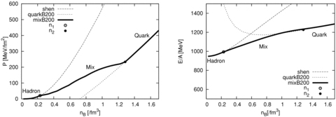
The constructed EOS under the bulk Gibbs condition. The labels of ‘quarkB200’ and ‘mixB200’ indicate a pure quark matter EOS and an EOS with a mixed phase with B= 200 MeV fm⁻³, respectively, whereas ‘Shen’ indicates the Shen EOS of pure hadronic matter. The left-hand and right-hand panels are the pressure and the energy per baryon as a function of the baryon number density, respectively.

Open in new tabDownload slide

Figure 2

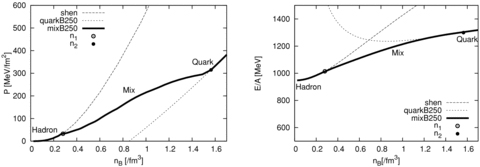
Same as Fig. 1 but for B= 250 MeV fm⁻³.

Open in new tabDownload slide

The actual conversion process from nuclear matter to quark matter, such as detonation or deflagration, has been a topic of hot debate (Drago, Lavagno & Parenti 2007). The range of the conversion time-scale is estimated to be very wide, roughly 0.1–100 s, depending upon the bag constant, temperature, mass of neutron stars and so on (Olesen & Madsen 1991). Since our main aim of this paper is the estimation of the liberated energy by the conversion from neutron stars to hybrid stars, we do not consider the detailed combustion processes in this study.

Protoneutron stars left after supernova explosion are initially very hot (∼50 MeV); however, they cool down below ∼1 MeV in some tens of seconds (Burrows & Lattimer 1986). The newly formed neutron stars stabilize at practically zero temperature. As mentioned, in cold neutron stars, the β-equilibrium in the weak interactions can be well validated, with neutrinos and antineutrinos freely escaping from the star. Combining the zero temperature, zero neutrino fraction and the β-equilibrium conditions with the charge neutrality condition, the thermodynamic variables depending on the three parameters [e.g. the pressure as P(ρ, Y_e, T) with Y_e being the electron fraction] can only be determined by a single variable (barotropic), which we take to be the energy density, namely P(ε) (Shapiro & Teukolsky 1983) in the following.

In the following, we introduce the baryon mass density, ρ₀, for convenience, defined to be the number density, n, multiplied by a baryon mass, m₀= 1.6605 × 10⁻²⁴ g.

2.2 Constructing the method of equilibrium stellar configurations

Employing the constructed EOS with the phase transition, we construct the equilibrium stellar configurations. As mentioned in Section 1, we pay attention to the general relativistic and toroidally magnetized stellar configurations. The basic equations and the numerical methods for this purpose are already given in Kiuchi & Yoshida (2008). Hence, we only give a brief summary for later convenience.

Assumptions to obtain the equilibrium models are summarized as follows. (1) Equilibrium models are stationary and axisymmetric. (2) The matter source is approximated by a perfect fluid with infinite conductivity. (3) There is no meridional flow of matter. (4) The EOS for the matter is barotropic, which is satisfied as mentioned. (5) The magnetic axis and rotation axis are aligned. Because the circularity condition (Wald 1984) holds under these assumptions, the metric can be written in the form (Komatsu, Eriguchi & Hachisu 1989a,b; Cook, Shapiro & Teukolsky 1992)

11

where the metric potentials, γ, ρ, α and ω, are functions of r and θ only. We see that the non-zero component of the Faraday tensor F_μν in this coordinate is F₁₂. Integrability of the equation of motion of the matter requires

12

where K is an arbitrary function of ρ₀he^2γr² sin²θ. The variables ρ₀ and h represent the baryon density and relativistic specific enthalpy, respectively. Integrating the equation of motion of the matter, we arrive at the equation of hydrostatic equilibrium:

13

where v= (Ω−ω)r sin θe^−ρ with Ω being the angular velocity of the matter and C is an integration constant. Here, we assume the rigid rotation. The first term of equation (13) depends only on EOSs. Hence, we prepare the values of the integral with EOS tables precisely. This preparation enables us to calculate equation (13) precisely, though our EOSs are quite different from polytropic models. To compute specific models of the magnetized stars, we need to specify the functional form of K, which determines the distribution of the magnetic fields. We take the following simple form:

14

where b and k are constants. Regularity of the toroidal magnetic field on the magnetic axis requires that k≥ 1. If k≥ 1, then the magnetic fields vanish at the surface of the star. In this study, we consider the k= 1 case because in the general relativistic MHD simulation, Kiuchi et al. (2008c) have found that magnetic distribution with k≠ 1 is unstable against axisymmetric perturbations.

To solve the master equations numerically, we employ the Cook–Shapiro–Teukolsky scheme (Cook et al. 1992) extended by Kiuchi & Yoshida (2008), which does not consider the functional form of the EOS. Hence, it is straightforward to update our numerical code for incorporating the EOS with the phase transition.

After obtaining solutions, it is useful to compute global physical quantities characterizing the equilibrium configurations to clearly understand the properties of the sequences of the equilibrium models. In this paper, we compute the following quantities: the gravitational mass M, the baryon rest mass M₀, the total angular momentum J, the total rotational energy T, the total magnetic energy H, the magnetic flux Φ, the gravitational energy W and the mean deformation rate ⁠, whose definitions are explicitly given in Kiuchi & Yoshida (2008). More explicitly, the mean deformation rate is defined as

15

where and with ε being the energy density of the matter. The circumferential radius R_cir is defined as R_cir≡ e^(γ−ρ)/2r_e with r_e being the coordinate radius at the stellar equatorial surface.

We checked the convergence of the presented results by doubling the mesh numbers from the standard set of radial and angular direction mesh points of 400 × 260. By checking the relativistic virial identities (Bonazzola & Gourgoulhon 1994) for all the models, we confirm that the typical values are of the orders of magnitude 10⁻³, and become 10⁻² at worse (10⁻⁴ at best). These values, which are a measure of the numerical convergence, are almost the same for the polytropic EOS case (Kiuchi & Yoshida 2008). In general, the convergence is known to become much worse for realistic EOSs, because their density and pressure profile are not smooth due to phase transitions. In this respect, our numerical scheme works well. In Section 3.2, we will discuss energy releases by the QCD phase transition and find that the values of our interest are ∼10⁻² M_⊙, for which the above numerical accuracy above is certificated mostly. By doubling the mesh points, i.e. 800(r) × 520(θ), we checked that the order of the magnitude of the released energy does not change.

In constructing one equilibrium sequence, we have three parameters to choose, namely the central density ρ_c, the strength of the magnetic field parameter b and the axial ratio r_p/r_e. Changing these parameters, we seek solutions in as wide a parameter range as possible for studying the properties of the equilibrium sequences. We need to calculate more than 50 models changing ρ_c, b, to follow one evolutionary sequence for a fixed baryon mass and magnetic flux. In addition, we change the initial angular momentum of each sequence by 10 models to model the rapidly rotating case to the non-rotating case, and three different EOSs of mixB200, mixB250 and Shen are also employed. This means that we have to construct at least 1500 models to explore the properties of the magnetized compact objects with quark cores systematically. In doing so, we use the Rosenbrock and Gram-Schmidt method, which is helpful in obtaining the convergence of the solutions efficiently.

3 NUMERICAL RESULTS

First of all, we discuss how the EOS with the phase transition affects the equilibrium configurations in Section 3.1, where we pay attention to non-rotating models. Since the magnetars and the high field neutron stars observed so far are all slow rotators, such non-rotating but highly magnetized static models could well be approximated to such stars. Moreover, the static models merit that one can see purely magnetic effects on the equilibrium properties because there is no centrifugal force and all the stellar deformation is attributed to the magnetic stress. Then in Section 3.2, we move on to discuss the releasable energy of the phase transition from the rotating and magnetized hadronic stars to the hybrid stars.

3.1 Effect of the phase transition on the equilibrium configurations

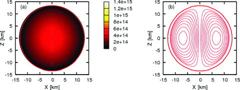
Now we discuss the equilibrium configurations of the non-rotating and strongly magnetized compact stars with/without the quark cores. Figs 3 and 4 are one example for the hybrid star with the mixB200 EOS and for the neutron star with the hadronic ‘Shen’ EOS, showing the distributions of the baryon density (left-hand panel) and the magnetic field (right-hand panel) in the meridional planes, respectively. These two models have the same baryon mass of 1.86 M_⊙, and the same magnetic flux of 2.00 × 10³⁰ G cm², which mean that they are really highly magnetized models with the central magnetic fields of ∼10¹⁸ G.

Figure 3

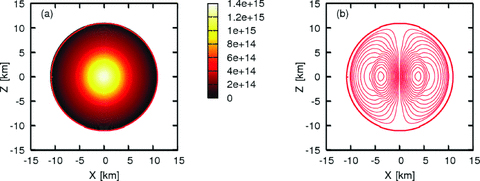
Distribution of (a) baryon density (g cm⁻³) and (b) magnetic field with the ‘mixB200’ EOS. Here, the central baryon density g cm⁻³, the baryon mass M₀= 1.86 M_⊙, the gravitational mass M= 1.69 M_⊙, the flux normalized by units of 10³⁰ G cm², Φ₃₀= 2.00, the ratio of the magnetic energy to the gravitational energy H/|W| = 1.65 × 10⁻², maximum magnetic fields B_max= 1.44 × 10¹⁸ G.

Open in new tabDownload slide

Figure 4

Same as Fig. 4 but for the hadronic ‘Shen’ EOS, M₀= 1.86 M_⊙ star with the central baryon density g cm⁻³, M= 1.71 M_⊙, H/|W| = 2.25 × 10⁻², B_max= 0.97 × 10¹⁸ G.

Open in new tabDownload slide

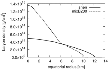
Comparing the left-hand panels of Figs 3 and 4, more concentration of the matter in the centre is clearly seen for the hybrid star (Fig. 3). The concentration is also clearly seen from Fig. 5. Inside the inner 6 km of the core of the hybrid star, the mixed phase appears, leading to the enhancement in the compression of the matter due to the softening of the EOS (e.g. Figs 1 and 2).

Figure 5

Distribution of the baryon density for Figs 3 and 4.

Open in new tabDownload slide

From the right-hand panel of Fig. 4, the strong toroidal field lines are seen to behave like a rubber belt, wrapping around the waist of the neutron star. It is found that the magnetic fields, frozen-in to the matter, are also compressed by the presence of the quark phase for the hybrid star (right-hand panel of Fig. 3). In fact, the pinching of the field lines in the panel corresponds to the surface of the quark core, ∼6 km in radius. These qualitative features are also true for the other equilibrium models.

In addition, a general trend in the equilibrium configurations for the hybrid stars is that they are more compact than the neutron star, due to the softness of the EOS. Given the same stellar baryon mass (M₀), the gravitational mass is smaller up to ∼0.01 M_⊙ than for the neutron stars, reflecting their smaller energy of the quark matter (right-hand panel of Fig. 1).

Given the fixed magnetic flux, we can construct equilibrium sequences by changing the central density. To characterize the features of the hybrid stars, we pay attention to the model with the maximum mass (dM/dρ_0,c= 0) along each sequence, which we call the maximum mass sequence for convenience. In Table 2, the important physical quantities are summarized for the maximum mass sequences with different magnetic fluxes. It is noted here that the maximum value of the magnetic flux in the table (Φ= 2.5 × 10³⁰ G cm²) corresponds to the non-convergence limit, beyond which any solutions cannot converge with the present numerical scheme (Kiuchi & Yoshida 2008). Albeit with such limitations, the field strength is already high enough to affect the configurations and we can well study the magnetic effects on them.

Table 2

Open in new tab

Global physical quantities for the maximum gravitational mass models of the constant magnetic flux sequences of the non-rotating stars. The order of EOSs from top to bottom indicates their hardness from the hadronic ‘Shen EOS’ to the softest ‘mixB200’ EOS.

Φ (1030 G cm2)	ρ0,c(1015 g cm−3)	M (M⊙)	M0(M⊙)	Rcir(km)	Bmax(1018 G)	H/|W|
Shen
0.00E+00	1.16E+00	2.46E+00	2.86E+00	1.35E+01	0.00E+00	0.00E+00	0.00E+00
1.50E+00	1.01E+00	2.45E+00	2.83E+00	1.39E+01	7.34E−01	3.81E−03	−7.40E−03
2.00E+00	1.05E+00	2.45E+00	2.84E+00	1.39E+01	9.83E−01	6.59E−03	−1.30E−02
2.50E+00	1.17E+00	2.46E+00	2.85E+00	1.36E+01	1.26E+00	9.48E−03	−1.86E−02
mixB250
0.00E+00	1.18E+00	1.83E+00	2.03E+00	1.47E+01	0.00E+00	0.00E+00	0.00E+00
1.50E+00	1.17E+00	1.83E+00	2.02E+00	1.40E+01	9.38E−01	8.28E−03	−1.97E−02
2.00E+00	1.18E+00	1.83E+00	2.02E+00	1.41E+01	1.23E+00	1.45E−02	−3.50E−02
2.50E+00	1.64E+00	1.82E+00	2.00E+00	1.33E+01	1.76E+00	2.02E−02	−63E−02
mixB200
0.00E+00	1.44E+00	1.70E+00	1.88E+00	1.30E+01	0.00E+00	0.00E+00	0.00E+00
1.50E+00	1.29E+00	1.69E+00	1.86E+00	1.34E+01	1.08E+00	9.62E−03	−2.25E−02
2.00E+00	1.35E+00	1.69E+00	1.86E+00	1.34E+01	1.44E+00	1.65E−02	−3.92E−02
2.50E+00	1.65E+00	1.69E+00	1.86E+00	1.31E+01	1.86E+00	2.39E−02	−5.59E−02

Φ (1030 G cm2)	ρ0,c(1015 g cm−3)	M (M⊙)	M0(M⊙)	Rcir(km)	Bmax(1018 G)	H/|W|
Shen
0.00E+00	1.16E+00	2.46E+00	2.86E+00	1.35E+01	0.00E+00	0.00E+00	0.00E+00
1.50E+00	1.01E+00	2.45E+00	2.83E+00	1.39E+01	7.34E−01	3.81E−03	−7.40E−03
2.00E+00	1.05E+00	2.45E+00	2.84E+00	1.39E+01	9.83E−01	6.59E−03	−1.30E−02
2.50E+00	1.17E+00	2.46E+00	2.85E+00	1.36E+01	1.26E+00	9.48E−03	−1.86E−02
mixB250
0.00E+00	1.18E+00	1.83E+00	2.03E+00	1.47E+01	0.00E+00	0.00E+00	0.00E+00
1.50E+00	1.17E+00	1.83E+00	2.02E+00	1.40E+01	9.38E−01	8.28E−03	−1.97E−02
2.00E+00	1.18E+00	1.83E+00	2.02E+00	1.41E+01	1.23E+00	1.45E−02	−3.50E−02
2.50E+00	1.64E+00	1.82E+00	2.00E+00	1.33E+01	1.76E+00	2.02E−02	−63E−02
mixB200
0.00E+00	1.44E+00	1.70E+00	1.88E+00	1.30E+01	0.00E+00	0.00E+00	0.00E+00
1.50E+00	1.29E+00	1.69E+00	1.86E+00	1.34E+01	1.08E+00	9.62E−03	−2.25E−02
2.00E+00	1.35E+00	1.69E+00	1.86E+00	1.34E+01	1.44E+00	1.65E−02	−3.92E−02
2.50E+00	1.65E+00	1.69E+00	1.86E+00	1.31E+01	1.86E+00	2.39E−02	−5.59E−02

Table 2

Open in new tab

Global physical quantities for the maximum gravitational mass models of the constant magnetic flux sequences of the non-rotating stars. The order of EOSs from top to bottom indicates their hardness from the hadronic ‘Shen EOS’ to the softest ‘mixB200’ EOS.

Φ (1030 G cm2)	ρ0,c(1015 g cm−3)	M (M⊙)	M0(M⊙)	Rcir(km)	Bmax(1018 G)	H/|W|
Shen
0.00E+00	1.16E+00	2.46E+00	2.86E+00	1.35E+01	0.00E+00	0.00E+00	0.00E+00
1.50E+00	1.01E+00	2.45E+00	2.83E+00	1.39E+01	7.34E−01	3.81E−03	−7.40E−03
2.00E+00	1.05E+00	2.45E+00	2.84E+00	1.39E+01	9.83E−01	6.59E−03	−1.30E−02
2.50E+00	1.17E+00	2.46E+00	2.85E+00	1.36E+01	1.26E+00	9.48E−03	−1.86E−02
mixB250
0.00E+00	1.18E+00	1.83E+00	2.03E+00	1.47E+01	0.00E+00	0.00E+00	0.00E+00
1.50E+00	1.17E+00	1.83E+00	2.02E+00	1.40E+01	9.38E−01	8.28E−03	−1.97E−02
2.00E+00	1.18E+00	1.83E+00	2.02E+00	1.41E+01	1.23E+00	1.45E−02	−3.50E−02
2.50E+00	1.64E+00	1.82E+00	2.00E+00	1.33E+01	1.76E+00	2.02E−02	−63E−02
mixB200
0.00E+00	1.44E+00	1.70E+00	1.88E+00	1.30E+01	0.00E+00	0.00E+00	0.00E+00
1.50E+00	1.29E+00	1.69E+00	1.86E+00	1.34E+01	1.08E+00	9.62E−03	−2.25E−02
2.00E+00	1.35E+00	1.69E+00	1.86E+00	1.34E+01	1.44E+00	1.65E−02	−3.92E−02
2.50E+00	1.65E+00	1.69E+00	1.86E+00	1.31E+01	1.86E+00	2.39E−02	−5.59E−02

Φ (1030 G cm2)	ρ0,c(1015 g cm−3)	M (M⊙)	M0(M⊙)	Rcir(km)	Bmax(1018 G)	H/|W|
Shen
0.00E+00	1.16E+00	2.46E+00	2.86E+00	1.35E+01	0.00E+00	0.00E+00	0.00E+00
1.50E+00	1.01E+00	2.45E+00	2.83E+00	1.39E+01	7.34E−01	3.81E−03	−7.40E−03
2.00E+00	1.05E+00	2.45E+00	2.84E+00	1.39E+01	9.83E−01	6.59E−03	−1.30E−02
2.50E+00	1.17E+00	2.46E+00	2.85E+00	1.36E+01	1.26E+00	9.48E−03	−1.86E−02
mixB250
0.00E+00	1.18E+00	1.83E+00	2.03E+00	1.47E+01	0.00E+00	0.00E+00	0.00E+00
1.50E+00	1.17E+00	1.83E+00	2.02E+00	1.40E+01	9.38E−01	8.28E−03	−1.97E−02
2.00E+00	1.18E+00	1.83E+00	2.02E+00	1.41E+01	1.23E+00	1.45E−02	−3.50E−02
2.50E+00	1.64E+00	1.82E+00	2.00E+00	1.33E+01	1.76E+00	2.02E−02	−63E−02
mixB200
0.00E+00	1.44E+00	1.70E+00	1.88E+00	1.30E+01	0.00E+00	0.00E+00	0.00E+00
1.50E+00	1.29E+00	1.69E+00	1.86E+00	1.34E+01	1.08E+00	9.62E−03	−2.25E−02
2.00E+00	1.35E+00	1.69E+00	1.86E+00	1.34E+01	1.44E+00	1.65E−02	−3.92E−02
2.50E+00	1.65E+00	1.69E+00	1.86E+00	1.31E+01	1.86E+00	2.39E−02	−5.59E−02

Since the compression of the matter is more enhanced for the smaller bag constant, the hybrid stars with the smaller bag constant become more compact (see R_cir in Table 2). The maximum magnetic fields are found to be up to about 30 per cent larger for the hybrid stars than for the neutron stars (compare B_max for mixB200 with B_max for Shen). It is also found that the hybrid stars with the smaller bag constant become more prolate (smaller values of ⁠) and also their maximum masses become smaller up to ∼10 per cent than those for the larger bag constant models. All these features are helpful in understanding the properties of the evolution tracks of the hybrid stars, which we discuss in the next section.

3.2 An evolutionary track to a hybrid star

Based on the equilibrium configurations mentioned above, we now move on to discuss an evolutionary path to the formation of a hybrid star due to the spin-down of magnetized and rotating neutron stars.

The evolution scenario we have in mind is illustrated in Fig. 6. Let us consider the evolution of a single protoneutron star, left after core-collapse supernova explosion, which rotates with the mass-shedding limit (A in Fig. 6). The maximum magnetic fields deep inside the core are taken to be ∼10¹⁸ G, which could be sustained due to α−Ω dynamos in such a rapidly rotating neutron star (Thompson & Duncan 1993, 1996). It should be noted that the possibility of such ultra-magnetic fields has not been rejected so far, because what we can learn from the observations of magnetars by their periods and spin-down rates is only their surface fields (∼10¹⁵ G). During their evolution, the baryon mass and the magnetic field strength are assumed to be constant for simplicity. Such models may model the evolution of the isolated compact stars, losing angular momentum via the gravitational radiation and/or magnetic breaking (from A to B). The phase transition to the hybrid stars is expected to take place during the evolution (shown as B to C in Fig. 6). At the moment, the baryon rest masses and the angular momenta are assumed to be conserved, which may be justified because the time-scale of the conversion, albeit uncertain of 0.1–100 s, are too short compared to the typical evolutionary time-scale of compact stars (more than 10³ yr; Olesen & Madsen 1991). After the transition, the newly born hybrid star evolves, again losing the angular momentum, to settle down to the magnetized and no-rotating hybrid star finally (see C to D).

Figure 6

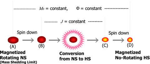
Schematic drawing, showing our scenario of conversion from neutron stars (NSs) to hybrid stars (HSs). The baryon rest mass and the magnetic flux are assumed to be conserved for modelling the isolated neutron stars that are adiabatically losing angular momentum via gravitational radiation and/or magnetic breaking. We furthermore assume the conservation of the angular momentum at the conversion.

Open in new tabDownload slide

Now using the left-hand panel of Fig. 7, we proceed to discuss quantitatively the evolution tracks mentioned above. The red solid line shows the baryon mass ‘M₀= 1.86 M_⊙’ rotating with the mass shedding limit (corresponding to A in Fig. 6). It is noted that the choice of the baryon mass (M₀= 1.86 M_⊙) is determined by the maximum mass of the non-rotating hybrid star with the mixB200 EOS as discussed in Section 3.1 and also that this baryon mass constant sequence has the largest releasable energy at the transition among all the models, as we will show later. There are many possible paths to convert to hybrid stars with different masses. However, we focused on the maximum energy release with the QCD phase transition in this paper. It is possible to select a single equilibrium sequence by keeping the baryon rest mass and the magnetic flux constant simultaneously. Thus, the evolution of the protoneutron star can be described along the line (pink dotted line), going right from one point on the red solid curve. As mentioned, our models assume that all equilibrium sequences begin at their mass-shedding limits and continue to non-rotating equilibrium hybrid stars, at which the sequences end. The final result is shown by the green dashed line in Fig. 7, which is the non-rotating hybrid star with the same baryon mass of ‘M₀= 1.86 M_⊙’, here for the mixB200 EOS (corresponding to D in Fig. 6).

Figure 7

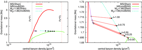
Gravitational masses versus central effective baryon densities at the constant magnetic flux, Φ₃₀= 2.00. The right-hand panel is a magnified figure of the left-hand panel. The solid line of MS (Shen) is for mass shedding limits of neutron stars. The dashed line of NR (mixB200) is for no-rotating hybrid stars with a ‘mixB200’ EOS. The line of ‘M₀= 1.86 (Shen)’ is one example in all baryon mass constant lines for neutron stars. ‘M₀= 1.86 (mixB200)’ is the same as ‘M₀= 1.86 (Shen)’, but for hybrid stars. Conversions from neutron stars to hybrid stars are shown as the vectors from a circle (○) to a filled circle (•). Here, J is the angular momentum in unit of 10⁴⁹ g cm² s⁻¹. The lines of ρ₁ and ρ₂ are critical densities of phase equilibrium for the hadron phase and quark phase shown in Fig. 1 and Table 1.

Open in new tabDownload slide

Between ρ₁ and ρ₂ (the vertical lines in Fig. 7), the phase transition should take place, producing a jump to the sequence of hybrid stars (from B to C in Fig. 6). In order to see clearly, the transition is shown as vectors from a circle (○) to a filled circle (•) in the right-hand panel of Fig. 7, which is just the magnification of the left-hand panel near the phase transition. Here, ‘J= 1.00’ (‘J= 0.70’, ‘J= 0.50’, ‘J= 0.25’) denotes the angular momentum in the unit of 10⁴⁹ g cm² s⁻¹. We estimate the energy release at the phase transition simply by the difference in the mass energies between the neutron star and the hybrid star:

16

by conserving Φ and J through the transition.

In Fig. 8, we show the releasable energy of ΔM as a function of the angular momentum for the mixB200 EOS. The top panel is for the baryon mass of M₀= 1.86 M_⊙, which is a special evolutionary track in the sense that the baryon mass is the maximum among non-rotating models, so that the releasable energy is largest among the computed models. Also for the other baryon mass models (middle and bottom panels), it is seen that the energy release becomes smaller for the larger angular momentum. This is simply because stronger centrifugal forces prevent the compression [see the central density (ρ_c) in Tables 3 and 4], making the quark cores smaller, which weakens the effect of the phase transition. In all the computed models, the maximum energy release is found to be ≲0.01 M_⊙. This energy is equivalent to ≲2 × 10⁵² erg, which is truly larger compared with the energies of supernovae (∼10⁵¹ erg); however, it is much smaller than those previously estimated (∼10⁵³ erg) in which the conversion to the strange quark star is assumed (Gourgoulhon et al. 1999; Yasutake et al. 2005; Zdunik et al. 2007). We note that ΔM becomes less than ΔM≲ 10⁻³ M_⊙ for the larger bag constant models of mixB250. This is because the large bag constant suppresses the conversion from hadron matter to quark matter as already mentioned. Unfortunately, exact values of ΔM for the mixB250 models cannot be found by the present scheme because ΔM becomes more than three orders-of-magnitude smaller than M, while M can be estimated at most with the numerical accuracy of 10⁻² for this case. This is also the case for small baryon mass cases (see the bottom panel of Fig. 8). For obtaining more precise solutions, we may need to employ the so-called spectral method. Although the lorene code (Bonazzola, Gourgoulhon & Marck 1998) employs the method, it however cannot treat the magnetic fields. The implementation of the method is still a major undertaking, which we consider as the next task of this paper.

Figure 8

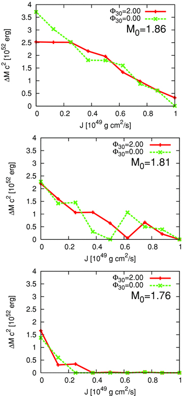
Energy release (ΔM) as a function of the angular momentum (J) at the moment of the phase transition for magnetized (Φ₃₀= 2.00) and non-magnetized models (Φ₃₀= 0) for M₀= 1.86 M_⊙ (the upper panel), M₀= 1.81 M_⊙ (the middle panel) and M₀= 1.76 M_⊙ (the lower panel). Note here that these are the case for the mixB200 EOS. For the mixB250 EOS, exact values of ΔM cannot be estimated due to the limitation of the present scheme. Unfortunately it is also seen here, for example, for the case of smaller baryon mass for J≳ 0.4 × 10⁴⁹ (g cm² s⁻¹) (bottom) (see text for more details).

Open in new tabDownload slide

Table 3

Open in new tab

Global physical quantities for the equilibrium sequences of the rotating stars with M₀= 1.86 M_⊙, Φ₃₀= 2.00.

EOS	ρ0,c(1015 g cm−3)	M (M⊙)	Rcir(km)	Ω (103 rad s−1)	T/|W|	H/|W|		Bmax(1018 G)
Shen(MS)	4.11E−01	1.73E+00	2.22E+01	1.59E+00	9.41E−02	2.89E−02	2.00E−01	9.61E−01
J= 1.00 ×1049 (g cm2) s−1
Shen	4.51E−01	1.72E+00	1.70E+01	8.73E−01	3.69E−02	2.47E−02	5.40E−02	9.65E−01
mixB250	5.11E−01	1.72E+00	1.69E+01	9.31E−01	3.65E−02	2.42E−02	5.40E−02	9.68E−01
mixB200	8.26E−01	1.71E+00	1.61E+01	1.30E+00	3.78E−02	2.11E−02	7.01E−02	1.10E+00
J= 0.75 ×1049 (g cm2) s−1
Shen	4.63E−01	1.71+00	1.64E+01	6.69E−01	2.15E−02	2.37E−02	7.26E−03	9.70E−01
mixB250	5.56E+00	1.71E+00	1.63E+01	7.40E−01	2.13E−02	2.33E−02	8.32E−03	9.74E−01
mixB200	9.63E−01	1.71E+00	1.51E+01	1.10E+00	2.24E−02	1.93E−02	2.74E−02	1.20E+00
J= 0.50 ×1049 (g cm2) s−1
Shen	4.72E−01	1.71E+00	1.60E+01	4.54E−01	9.83E−03	2.31E−02	−3.05E−02	9.70E−01
mixB250	5.93E−01	1.71E+00	1.59E+01	5.16E−01	9.77E−03	2.24E−02	−2.82E−02	9.75E−01
mixB200	1.08E+00	1.70E+00	1.43E+01	8.07E−01	1.04E−02	1.81E−02	−8.49E−03	1.31E+00
J= 0.25 ×1049 (g cm2) s−1
Shen	4.79E−01	1.71E+00	1.58E+01	2.28E−01	4.53E−03	2.28E−02	−4.82E−02	9.70E−01
mixB250	6.15E−01	1.71E+00	1.57E+01	2.60E−01	4.43E−03	2.20E−02	−4.57E−02	9.75E−01
mixB200	1.21E+00	1.69E+00	1.42E+01	4.39E−01	2.82E−03	1.71E−02	−3.15E−02	1.39E+00
No rotation
Shen	4.86E−01	1.71E+00	1.57E+01	0.00E+00	0.00E+00	2.25E−02	−6.35E−02	9.72E−01
mixB250	6.36E−01	1.71E+00	1.55E+01	0.00E+00	0.00E+00	2.16E−02	−6.03E−02	9.75E−01
mixB200	1.35E+00	1.69E+00	1.34E+01	0.00E+00	0.00E+00	1.65E−02	−3.92E−02	1.44E+00

EOS	ρ0,c(1015 g cm−3)	M (M⊙)	Rcir(km)	Ω (103 rad s−1)	T/|W|	H/|W|		Bmax(1018 G)
Shen(MS)	4.11E−01	1.73E+00	2.22E+01	1.59E+00	9.41E−02	2.89E−02	2.00E−01	9.61E−01
J= 1.00 ×1049 (g cm2) s−1
Shen	4.51E−01	1.72E+00	1.70E+01	8.73E−01	3.69E−02	2.47E−02	5.40E−02	9.65E−01
mixB250	5.11E−01	1.72E+00	1.69E+01	9.31E−01	3.65E−02	2.42E−02	5.40E−02	9.68E−01
mixB200	8.26E−01	1.71E+00	1.61E+01	1.30E+00	3.78E−02	2.11E−02	7.01E−02	1.10E+00
J= 0.75 ×1049 (g cm2) s−1
Shen	4.63E−01	1.71+00	1.64E+01	6.69E−01	2.15E−02	2.37E−02	7.26E−03	9.70E−01
mixB250	5.56E+00	1.71E+00	1.63E+01	7.40E−01	2.13E−02	2.33E−02	8.32E−03	9.74E−01
mixB200	9.63E−01	1.71E+00	1.51E+01	1.10E+00	2.24E−02	1.93E−02	2.74E−02	1.20E+00
J= 0.50 ×1049 (g cm2) s−1
Shen	4.72E−01	1.71E+00	1.60E+01	4.54E−01	9.83E−03	2.31E−02	−3.05E−02	9.70E−01
mixB250	5.93E−01	1.71E+00	1.59E+01	5.16E−01	9.77E−03	2.24E−02	−2.82E−02	9.75E−01
mixB200	1.08E+00	1.70E+00	1.43E+01	8.07E−01	1.04E−02	1.81E−02	−8.49E−03	1.31E+00
J= 0.25 ×1049 (g cm2) s−1
Shen	4.79E−01	1.71E+00	1.58E+01	2.28E−01	4.53E−03	2.28E−02	−4.82E−02	9.70E−01
mixB250	6.15E−01	1.71E+00	1.57E+01	2.60E−01	4.43E−03	2.20E−02	−4.57E−02	9.75E−01
mixB200	1.21E+00	1.69E+00	1.42E+01	4.39E−01	2.82E−03	1.71E−02	−3.15E−02	1.39E+00
No rotation
Shen	4.86E−01	1.71E+00	1.57E+01	0.00E+00	0.00E+00	2.25E−02	−6.35E−02	9.72E−01
mixB250	6.36E−01	1.71E+00	1.55E+01	0.00E+00	0.00E+00	2.16E−02	−6.03E−02	9.75E−01
mixB200	1.35E+00	1.69E+00	1.34E+01	0.00E+00	0.00E+00	1.65E−02	−3.92E−02	1.44E+00

Table 3

Open in new tab

Global physical quantities for the equilibrium sequences of the rotating stars with M₀= 1.86 M_⊙, Φ₃₀= 2.00.

EOS	ρ0,c(1015 g cm−3)	M (M⊙)	Rcir(km)	Ω (103 rad s−1)	T/|W|	H/|W|		Bmax(1018 G)
Shen(MS)	4.11E−01	1.73E+00	2.22E+01	1.59E+00	9.41E−02	2.89E−02	2.00E−01	9.61E−01
J= 1.00 ×1049 (g cm2) s−1
Shen	4.51E−01	1.72E+00	1.70E+01	8.73E−01	3.69E−02	2.47E−02	5.40E−02	9.65E−01
mixB250	5.11E−01	1.72E+00	1.69E+01	9.31E−01	3.65E−02	2.42E−02	5.40E−02	9.68E−01
mixB200	8.26E−01	1.71E+00	1.61E+01	1.30E+00	3.78E−02	2.11E−02	7.01E−02	1.10E+00
J= 0.75 ×1049 (g cm2) s−1
Shen	4.63E−01	1.71+00	1.64E+01	6.69E−01	2.15E−02	2.37E−02	7.26E−03	9.70E−01
mixB250	5.56E+00	1.71E+00	1.63E+01	7.40E−01	2.13E−02	2.33E−02	8.32E−03	9.74E−01
mixB200	9.63E−01	1.71E+00	1.51E+01	1.10E+00	2.24E−02	1.93E−02	2.74E−02	1.20E+00
J= 0.50 ×1049 (g cm2) s−1
Shen	4.72E−01	1.71E+00	1.60E+01	4.54E−01	9.83E−03	2.31E−02	−3.05E−02	9.70E−01
mixB250	5.93E−01	1.71E+00	1.59E+01	5.16E−01	9.77E−03	2.24E−02	−2.82E−02	9.75E−01
mixB200	1.08E+00	1.70E+00	1.43E+01	8.07E−01	1.04E−02	1.81E−02	−8.49E−03	1.31E+00
J= 0.25 ×1049 (g cm2) s−1
Shen	4.79E−01	1.71E+00	1.58E+01	2.28E−01	4.53E−03	2.28E−02	−4.82E−02	9.70E−01
mixB250	6.15E−01	1.71E+00	1.57E+01	2.60E−01	4.43E−03	2.20E−02	−4.57E−02	9.75E−01
mixB200	1.21E+00	1.69E+00	1.42E+01	4.39E−01	2.82E−03	1.71E−02	−3.15E−02	1.39E+00
No rotation
Shen	4.86E−01	1.71E+00	1.57E+01	0.00E+00	0.00E+00	2.25E−02	−6.35E−02	9.72E−01
mixB250	6.36E−01	1.71E+00	1.55E+01	0.00E+00	0.00E+00	2.16E−02	−6.03E−02	9.75E−01
mixB200	1.35E+00	1.69E+00	1.34E+01	0.00E+00	0.00E+00	1.65E−02	−3.92E−02	1.44E+00

EOS	ρ0,c(1015 g cm−3)	M (M⊙)	Rcir(km)	Ω (103 rad s−1)	T/|W|	H/|W|		Bmax(1018 G)
Shen(MS)	4.11E−01	1.73E+00	2.22E+01	1.59E+00	9.41E−02	2.89E−02	2.00E−01	9.61E−01
J= 1.00 ×1049 (g cm2) s−1
Shen	4.51E−01	1.72E+00	1.70E+01	8.73E−01	3.69E−02	2.47E−02	5.40E−02	9.65E−01
mixB250	5.11E−01	1.72E+00	1.69E+01	9.31E−01	3.65E−02	2.42E−02	5.40E−02	9.68E−01
mixB200	8.26E−01	1.71E+00	1.61E+01	1.30E+00	3.78E−02	2.11E−02	7.01E−02	1.10E+00
J= 0.75 ×1049 (g cm2) s−1
Shen	4.63E−01	1.71+00	1.64E+01	6.69E−01	2.15E−02	2.37E−02	7.26E−03	9.70E−01
mixB250	5.56E+00	1.71E+00	1.63E+01	7.40E−01	2.13E−02	2.33E−02	8.32E−03	9.74E−01
mixB200	9.63E−01	1.71E+00	1.51E+01	1.10E+00	2.24E−02	1.93E−02	2.74E−02	1.20E+00
J= 0.50 ×1049 (g cm2) s−1
Shen	4.72E−01	1.71E+00	1.60E+01	4.54E−01	9.83E−03	2.31E−02	−3.05E−02	9.70E−01
mixB250	5.93E−01	1.71E+00	1.59E+01	5.16E−01	9.77E−03	2.24E−02	−2.82E−02	9.75E−01
mixB200	1.08E+00	1.70E+00	1.43E+01	8.07E−01	1.04E−02	1.81E−02	−8.49E−03	1.31E+00
J= 0.25 ×1049 (g cm2) s−1
Shen	4.79E−01	1.71E+00	1.58E+01	2.28E−01	4.53E−03	2.28E−02	−4.82E−02	9.70E−01
mixB250	6.15E−01	1.71E+00	1.57E+01	2.60E−01	4.43E−03	2.20E−02	−4.57E−02	9.75E−01
mixB200	1.21E+00	1.69E+00	1.42E+01	4.39E−01	2.82E−03	1.71E−02	−3.15E−02	1.39E+00
No rotation
Shen	4.86E−01	1.71E+00	1.57E+01	0.00E+00	0.00E+00	2.25E−02	−6.35E−02	9.72E−01
mixB250	6.36E−01	1.71E+00	1.55E+01	0.00E+00	0.00E+00	2.16E−02	−6.03E−02	9.75E−01
mixB200	1.35E+00	1.69E+00	1.34E+01	0.00E+00	0.00E+00	1.65E−02	−3.92E−02	1.44E+00

Table 4

Open in new tab

Same as Table 3 but for Φ₃₀= 0.

EOS	ρ0,c(1015 g cm−3)	M (M⊙)	Rcir(km)	Ω (103 rad s−1)	T/|W|
Shen(MS)	3.81E−01	1.74E+00	2.10E+01	1.45E+00	1.12E−01	2.79E−01
J= 1.00 ×1049 (g cm2) s−1
Shen	4.40E−01	1.72E+00	1.66E+01	8.08E−01	3.58E−02	1.07E−01
mixB250	4.62E−01	1.72E+00	1.66E+01	8.30E−01	3.54E−02	1.06E−01
mixB200	7.80E−01	1.71E+00	1.58E+01	1.18E+00	3.72E−02	1.11E−01
J= 0.75 ×1049 (g cm2) s−1
Shen	4.51E−01	1.71E+00	1.61E+01	6.23E−01	2.09E−02	6.49E−02
mixB250	5.16E−01	1.71E+00	1.61E+01	6.69E−01	2.07E−02	6.43E−02
mixB200	9.02E−01	1.70E+00	1.49E+01	1.01E+00	2.18E−02	6.90E−02
J= 0.50 ×1049 (g cm2) s−1
Shen	4.61E−01	1.71E+00	1.58E+01	4.25E−01	9.54E−03	3.06E−02
mixB250	5.51E−01	1.71E+00	1.57E+01	4.69E−01	9.49E−03	3.04E−02
mixB200	1.03E+00	1.70E+00	1.42E+01	7.51E−01	1.02E−02	3.33E−02
J= 0.25 ×1049 (g cm2) s−1
Shen	4.67E−01	1.71E+00	1.56E+01	2.15E−01	2.54E−03	8.48E−03
mixB250	5.74E−01	1.71E+00	1.55E+01	2.42E−01	2.52E−03	8.46E−03
mixB200	1.14E+00	1.69E+00	1.37E+01	4.08E−01	2.65E−03	9.10E−03
No rotation
Shen	4.75E−01	1.71E+00	1.55E+01	0.00E+00	0.00E+00	0.00E+00
mixB250	5.82E−01	1.71E+00	1.54E+01	0.00E+00	0.00E+00	0.00E+00
mixB200	1.19E+00	1.69E+00	1.35E+01	0.00E+00	0.00E+00	0.00E+00

EOS	ρ0,c(1015 g cm−3)	M (M⊙)	Rcir(km)	Ω (103 rad s−1)	T/|W|
Shen(MS)	3.81E−01	1.74E+00	2.10E+01	1.45E+00	1.12E−01	2.79E−01
J= 1.00 ×1049 (g cm2) s−1
Shen	4.40E−01	1.72E+00	1.66E+01	8.08E−01	3.58E−02	1.07E−01
mixB250	4.62E−01	1.72E+00	1.66E+01	8.30E−01	3.54E−02	1.06E−01
mixB200	7.80E−01	1.71E+00	1.58E+01	1.18E+00	3.72E−02	1.11E−01
J= 0.75 ×1049 (g cm2) s−1
Shen	4.51E−01	1.71E+00	1.61E+01	6.23E−01	2.09E−02	6.49E−02
mixB250	5.16E−01	1.71E+00	1.61E+01	6.69E−01	2.07E−02	6.43E−02
mixB200	9.02E−01	1.70E+00	1.49E+01	1.01E+00	2.18E−02	6.90E−02
J= 0.50 ×1049 (g cm2) s−1
Shen	4.61E−01	1.71E+00	1.58E+01	4.25E−01	9.54E−03	3.06E−02
mixB250	5.51E−01	1.71E+00	1.57E+01	4.69E−01	9.49E−03	3.04E−02
mixB200	1.03E+00	1.70E+00	1.42E+01	7.51E−01	1.02E−02	3.33E−02
J= 0.25 ×1049 (g cm2) s−1
Shen	4.67E−01	1.71E+00	1.56E+01	2.15E−01	2.54E−03	8.48E−03
mixB250	5.74E−01	1.71E+00	1.55E+01	2.42E−01	2.52E−03	8.46E−03
mixB200	1.14E+00	1.69E+00	1.37E+01	4.08E−01	2.65E−03	9.10E−03
No rotation
Shen	4.75E−01	1.71E+00	1.55E+01	0.00E+00	0.00E+00	0.00E+00
mixB250	5.82E−01	1.71E+00	1.54E+01	0.00E+00	0.00E+00	0.00E+00
mixB200	1.19E+00	1.69E+00	1.35E+01	0.00E+00	0.00E+00	0.00E+00

Table 4

Open in new tab

Same as Table 3 but for Φ₃₀= 0.

EOS	ρ0,c(1015 g cm−3)	M (M⊙)	Rcir(km)	Ω (103 rad s−1)	T/|W|
Shen(MS)	3.81E−01	1.74E+00	2.10E+01	1.45E+00	1.12E−01	2.79E−01
J= 1.00 ×1049 (g cm2) s−1
Shen	4.40E−01	1.72E+00	1.66E+01	8.08E−01	3.58E−02	1.07E−01
mixB250	4.62E−01	1.72E+00	1.66E+01	8.30E−01	3.54E−02	1.06E−01
mixB200	7.80E−01	1.71E+00	1.58E+01	1.18E+00	3.72E−02	1.11E−01
J= 0.75 ×1049 (g cm2) s−1
Shen	4.51E−01	1.71E+00	1.61E+01	6.23E−01	2.09E−02	6.49E−02
mixB250	5.16E−01	1.71E+00	1.61E+01	6.69E−01	2.07E−02	6.43E−02
mixB200	9.02E−01	1.70E+00	1.49E+01	1.01E+00	2.18E−02	6.90E−02
J= 0.50 ×1049 (g cm2) s−1
Shen	4.61E−01	1.71E+00	1.58E+01	4.25E−01	9.54E−03	3.06E−02
mixB250	5.51E−01	1.71E+00	1.57E+01	4.69E−01	9.49E−03	3.04E−02
mixB200	1.03E+00	1.70E+00	1.42E+01	7.51E−01	1.02E−02	3.33E−02
J= 0.25 ×1049 (g cm2) s−1
Shen	4.67E−01	1.71E+00	1.56E+01	2.15E−01	2.54E−03	8.48E−03
mixB250	5.74E−01	1.71E+00	1.55E+01	2.42E−01	2.52E−03	8.46E−03
mixB200	1.14E+00	1.69E+00	1.37E+01	4.08E−01	2.65E−03	9.10E−03
No rotation
Shen	4.75E−01	1.71E+00	1.55E+01	0.00E+00	0.00E+00	0.00E+00
mixB250	5.82E−01	1.71E+00	1.54E+01	0.00E+00	0.00E+00	0.00E+00
mixB200	1.19E+00	1.69E+00	1.35E+01	0.00E+00	0.00E+00	0.00E+00

EOS	ρ0,c(1015 g cm−3)	M (M⊙)	Rcir(km)	Ω (103 rad s−1)	T/|W|
Shen(MS)	3.81E−01	1.74E+00	2.10E+01	1.45E+00	1.12E−01	2.79E−01
J= 1.00 ×1049 (g cm2) s−1
Shen	4.40E−01	1.72E+00	1.66E+01	8.08E−01	3.58E−02	1.07E−01
mixB250	4.62E−01	1.72E+00	1.66E+01	8.30E−01	3.54E−02	1.06E−01
mixB200	7.80E−01	1.71E+00	1.58E+01	1.18E+00	3.72E−02	1.11E−01
J= 0.75 ×1049 (g cm2) s−1
Shen	4.51E−01	1.71E+00	1.61E+01	6.23E−01	2.09E−02	6.49E−02
mixB250	5.16E−01	1.71E+00	1.61E+01	6.69E−01	2.07E−02	6.43E−02
mixB200	9.02E−01	1.70E+00	1.49E+01	1.01E+00	2.18E−02	6.90E−02
J= 0.50 ×1049 (g cm2) s−1
Shen	4.61E−01	1.71E+00	1.58E+01	4.25E−01	9.54E−03	3.06E−02
mixB250	5.51E−01	1.71E+00	1.57E+01	4.69E−01	9.49E−03	3.04E−02
mixB200	1.03E+00	1.70E+00	1.42E+01	7.51E−01	1.02E−02	3.33E−02
J= 0.25 ×1049 (g cm2) s−1
Shen	4.67E−01	1.71E+00	1.56E+01	2.15E−01	2.54E−03	8.48E−03
mixB250	5.74E−01	1.71E+00	1.55E+01	2.42E−01	2.52E−03	8.46E−03
mixB200	1.14E+00	1.69E+00	1.37E+01	4.08E−01	2.65E−03	9.10E−03
No rotation
Shen	4.75E−01	1.71E+00	1.55E+01	0.00E+00	0.00E+00	0.00E+00
mixB250	5.82E−01	1.71E+00	1.54E+01	0.00E+00	0.00E+00	0.00E+00
mixB200	1.19E+00	1.69E+00	1.35E+01	0.00E+00	0.00E+00	0.00E+00

Other numerical values characterizing the phase transition are given in Tables 3 and 4. Table 4 is for the non-magnetized models, which is given for comparison. For models with smaller angular momentum (J in the tables), it can be readily seen that the gravitational masses (M) and the circumferential radii (R_cir) become smaller, while the central baryon densities (ρ_0,c) and the maximum strength of the magnetic fields (B_max) become larger, all simply due to the smaller centrifugal forces. If the newly born neutron star evolves to the non-rotating neutron star without experiencing the conversion, then the increase in the central density is less than ∼20 per cent (compare ρ_0,c of ‘Shen’ at the mass shedding limit with that at the no-rotating limit in Table 3). On the other hand, the maximum density is found to increase about several times larger by the phase transition (compare ρ_0,c of ‘Shen’ with ‘mixB200’ in Table 3). Frozen-in to the matter, the maximum magnetic field increases up to 50 per cent while the change is an order of unit per cent in absence of the conversion (see Fig. 9). Due to the conservation of angular momentum, the angular velocity increases by about ΔΩ/Ω∼ 30 per cent after the conversion (see Fig. 10 and Table 3). Also in this case, it is noted that the spin-up is suppressed for the larger bag constant models (see Table 3). We speculate that such spin-up, much larger than the canonical glitches of magnetars (ΔΩ/Ω∼ 10⁻⁷; Woods & Thompson 2006), could be new observable signatures, marking the occurrence of the phase transition.

Figure 9

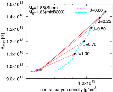
Central baryon density versus maximum magnetic field for the same stars of Fig. 7.

Open in new tabDownload slide

Figure 10

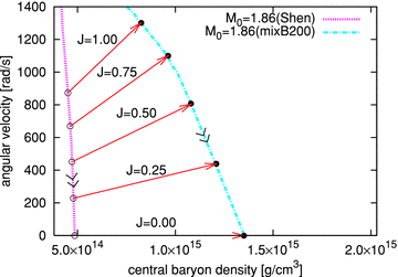
Central baryon density versus angular velocities for the same stars of Fig. 7. Angular velocities are monotonically decreased without the conversion, shown as ‘>>’.

Open in new tabDownload slide

4 SUMMARY AND DISCUSSION

In this study, we investigated the structures of general relativistic hybrid stars containing super-strong magnetic fields. Pushed by the results of recent stellar evolution calculations and the outcomes of recent MHD simulations of core-collapse supernovae, we treated the toroidal fields only. Using the bulk Gibbs construction, we modelled the EOS with a first-order transition by bridging the MIT bag model for the description of quark matter and the nuclear EOS by Shen et al. We found that the presence of the quark phase can affect the distribution of the magnetic fields inside the hybrid stars, leading to the enhancement of the field strength by about 30 per cent than for the normal neutron stars. Using the equilibrium configurations, we explored the possible evolutionary paths to the formation of hybrid stars due to the spin-down of magnetized and rotating neutron stars. For simplicity, the total baryon mass and magnetic flux are taken to be conserved during the evolution but the angular momenta are lost gravitational waves and/or magnetic breaking. We found that the energy release by the conversion to hybrid stars is typically ⁠, which is smaller than that previously estimated for the conversion to the strange quark stars.

In association with the vast energy release, it is natural to expect the emissions of gravitational waves. The amplitude of the gravitational waves associated with the phase transition, h, is given as (Pacheco 1998)

17

Here, E_tot, α, τ, r and ω are the energy release, fraction of the energy release emitted in the form of the gravitational waves, damping time-scale of the gravitational wave, distance to the source and angular velocity, respectively. To set an absolute upper bound, we could choose E_tot∼ 10⁵² erg and ω∼ 100 rad s⁻¹ according to Table 3. We assume that the source is in our Galactic Centre of r∼ 10 kpc and that the damping time-scale and α are ∼100 ms and 10⁻⁴, respectively, inferred from Abdikamalov et al. (2008). The resulting amplitudes become as high as h∼ 10^{−18∼−19} peaking at ∼kHz, which are surely within the detection limits for the laser interferometers in line such as LIGO, VIRGO, GEO600 and TAMA300. Considering the optimal sensitivity of the interferometers of h∼ 10⁻²¹ at ∼1 kHz, such signals, far stronger than those from canonical core-collapse supernovae (e.g. Kotake et al. 2009a,b; Murphy, Ott & Burrows 2009), are possibly visible for a source out to megaparsec distances. In combination with the signatures of the spin-up discussed before, we speculate that the waveforms of such strong gravitational waves could provide us hints of the properties of the QCD phase transition. To find the accurate waveforms, general relativistic simulations are indispensable (Kiuchi et al. in preparation). Moreover, accurate predictions for neutrino emissions (Gentile et al. 1993; Nakazato et al. 2008; Sagert et al. 2009) and their detectability still remain to be studied (e.g. Kawagoe, Takiwaki & Kotake 2009). This paper should help in constructing the initial conditions for such studies.

Alcock et al. (1986) claimed that the conversion from the hadronic to the mixed phase occurs instantaneously in the weak interaction time-scales (such as d+u ↔ s+u) when the central density exceeds the critical value of ρ₁ in Figs 1 and 2. If so, the newly born neutron stars may convert to the hybrid stars in the post-bounce phase, before they evolve from A to B illustrated in Fig. 6. In this case, the released energy may be used to power original core-collapse supernovae or more energetic supernovae such as hypernovae. Although the formation paths to hybrid stars are different from the ones discussed in this paper, the estimation method of the energy release here is also applicable if we implement the EOS at finite temperature and high lepton fraction (Yasutake & Kashiwa 2009), which we plan to study as a sequel to this paper.

It has been pointed out that the super-strong magnetic field more than 10¹⁸ G can affect the stiffness of the EOS (Broderick, Prakash & Lattimer 2000). As mentioned, the maximum magnetic field increases by about ∼30 per cent by the phase transition, while it increases by only a unit per cent if the compact stars evolve to the non-rotating ones in absence of the transition. This suggests that the magnetic effects should be seriously taken into account for our models treating the phase transition. Especially for the quark phase, Fukushima & Warringa (2008) and Noronha & Shovkovy (2007) have recently found that the energy gaps of the magnetic colour-flavour-locked phase are oscillating functions of the magnetic field. Such effects remain to be studied.

We should comment about the very high values of the magnetic fields, larger than 10¹⁸ G. Ruderman, Tao & Kluzníak (2000) suggested that such high magnetic fields can be brought to the stellar surface by buoyancy forces. According to their result, we estimate the buoyancy time-scale in our models. The buoyancy force can be expressed as

18

where c_s and g are the sound speed and the gravitational acceleration, respectively. Putting typical values inside compact objects into the equation, we roughly estimate the time-scale τ as

19

where R is the typical size of compact stars. Clearly, such magnetic fields are not stable against the buoyancy forces in a stellar evolution time-scale of ∼10³ yr. Based on the MHD simulations in full general relativity, Kiuchi et al. (2008c) recently showed that the toroidal configurations of neutron stars are really dynamically unstable due to the buoyant instability. But a more important finding relevant to this study is that the toroidal magnetic fields settle down to a new equilibrium state with the circular motions in the meridian plane. In the new equilibrium configurations, the toroidal fields almost equivalent to the strength before the onset of the instability are expected to be much stronger that the poloidal ones. This suggests that our models presented here, albeit unstable to the buoyant instability, could be helpful in understanding the equilibrium configurations of magnetized hybrid stars. Such stability analysis is an important issue yet to be studied.

Our treatments of the phase transition should be more sophisticated. We plan to employ the so-called NJL model (e.g. Yasutake & Kashiwa 2009) instead of the simple MIT bag model. Moreover, we shall take into account the finite size effects (Maruyama et al. 2006) such as quark-nuclear pasta structures. We considered cold compact objects, namely with zero temperature and zero neutrino fraction. We plan to extend this study to the finite temperature with the non-zero neutrino fraction, which should be useful for studying the earlier evolutions of compact stars soon after their formation.

The evolution sequence we explored is a very simplified one. For more realistic estimations, one needs the two-dimensional evolutionary calculation in a full general relativistic framework, which is not an easy job, due to the treatment of convection, combustion, cooling and/or heating processes, nucleosynthesis on the surface and so on. Applying the method recently reported by Pons, Miralles & Geppert (2009), we think that we could study the magnetothermal evolution of neutron stars to the hybrid stars. By doing so, we hope to investigate the peculiar properties in the light curves, which has been pointed out to be observationally visible (Blaschke, Klahn & Voskresensky 2000; Page et al. 2000; Blaschke, Grigorian & Voskresensky 2001; Grigorian, Blaschke & Voskresensky 2005). All such studies should be indispensable to pave the way for the understanding of the long-veiled phase-transition physics from the astrophysical phenomena.

We are grateful to Shijun Yoshida, Y. Eriguchi and M. Hashimoto, for informative discussions. NY thanks to Y. Sekiguchi for stimulating discussions. K. Kotake is grateful to K. Sato and S. Yamada for continuing encouragements. Numerical computations were in part carried on the XT4 general common use computer system at the Center for Computational Astrophysics, CfCA, the National Astronomical Observatory of Japan. This study was supported in part by the Grants-in-Aid for the Scientific Research from the Ministry of Education, Science and Culture of Japan (no. S19104006, 20740150, 21105512).

REFERENCES