


Abstract
An example of a cold massive core, JCMT 18354−0649S which is a possible high-mass analogue to a low-mass star-forming core, is studied. Line and continuum observations from James Clerk Maxwell Telescope, Mopra Telescope and Spitzer are presented and modelled in detail using a 3D molecular line radiative transfer code. In almost every way, JCMT 18354−0649S is a scaled-up version of a typical low-mass core with similar temperatures, chemical abundances and densities. The difference is that both the infall velocity and the turbulent width of the line profiles are an order of magnitude larger. While the higher infall velocity is expected due to the large mass of JCMT 18354−0649S, we suggest that the dissipation of this highly supersonic turbulence may lead to the creation of dense clumps of gas that surround the high-mass core.
1 INTRODUCTION
Studies of the formation of individual stars have traditionally distinguished between low-mass star formation and massive star formation. Low-mass stars tend to form in isolation in relatively quiescent environments such as those seen in Taurus. In massive star formation, such as in the Orion nebula, dense clusters of thousands of low-mass stars form alongside a few high-mass stars (>8 M⊙) which are capable of ionizing the surrounding remnant cloud. While the outcomes of these two modes of star formation are vastly different, evidence is growing that the physical conditions in the initial parent molecular clouds may be very similar, differing only in size and mass scale between the two paths (Hillenbrand & Hartmann 1998; Patel et al. 2005; Fontani et al. 2006).
A key question that remains is how and when massive star formation diverges from low-mass star formation. In order to address this problem, searches have been made for the high-mass equivalents of the starless or early protostellar cores seen in low-mass star formation (see Bacmann et al. 2000; André et al. 2004; Bergin & Tafalla 2007, for reviews). Infrared dark clouds, which are seen in absorption against 8 μm emission towards the Galactic Centre (Egan et al. 1998; Perault, Omont & Simon 1996; Teyssier, Hennebelle & Pérault 2002), are potential sites for massive star-forming clusters within which individual ‘cold massive cores’ can be identified. Another strategy is to search for cold massive cores amidst ongoing massive star formation (Garay et al. 2004; Hill et al. 2005; Pillai et al. 2007). Three examples of individual cold massive cores found via their dust continuum emission are JCMT 18354−0649S (Wu et al. 2005), G333.125−0.562 (Lo et al. 2007) and ISOSS J18364−0221 (Birkmann, Krause & Lemke 2006). The continuum emission indicates that these sources are cold (∼20 K) yet massive (800 M⊙, 1.8 × 10³ M⊙ and 75 M⊙, respectively) and thus are potential future sites of massive star formation.
Different molecular lines trace different parts of a cloud and an ideal tracer should faithfully trace the gas dynamics as deeply into the cloud as possible. Candidate dynamical tracer species include N2H+, HCO+, HCN, NH3 and CO amongst others. The interpretation of such lines is not trivial even with a radiative transfer code since effects such as depletion (when an atom/molecule freezes on to the surface of a dust grain) and chemical variation coupled with dynamics such as rotation, infall and outflow all contribute to the final emergent line profile. Progress becomes possible however if several lines from different species are used together.
Wu et al. (2005) observed JCMT 18354−0649S (hereafter JCMT 18354S) in four species using the James Clark Maxwell Telescope (JCMT): H13 CO+ (J= 3–2), C17 O (J= 2–1), HCO+ (J= 3–2). They found that the molecular line profiles look similar in shape to those of their low-mass counterparts (see also Fuller, Williams & Sridharan 2005). The main difference is in the line widths which are clearly broader. The linewidth at half the intensity for the lines C18O (2–1), C17O (2–1) and H13CO+ (3–2) are 4.03, 3.78 and 3.24, respectively. Comparing these values with the same parameters measured from the low-mass core L483 (Carolan et al. 2008), we find that the linewidths are 0.86, 1.09 and 0.66. This is a factor of 4 smaller than the linewidth in our high-mass core. Wu et al. (2005) showed that JCMT 18354S exhibits distinct blue–red asymmetries in the optically thick HCO+ and HCN lines, both known to be good tracers of infalling motions in low-mass star formation regions. A semi-analytic treatment of the radiative transfer led them to conclude that the densities, velocities and velocity dispersions implied by the observations are, as to be expected, much larger than for low-mass sources.
Previous observations by Wu et al. (2005) determined that JCMT 18354S core has a size of 10 arcsec corresponding to 0.28 pc at a distance of 5700 pc away with a vlsr of 95 km s−1. The total mass is 910 M⊙ and 820 M⊙ when derived from 850 μm and 450 μm emission. The dust temperature was estimated as Td= 14.4 K by fitting a grey body to the observed spectral energy distribution (SED) and assuming a dust emissivity index of β= 2 (Wu et al. 2005). However, the dust temperature ranges from 11 to 29 K when uncertainties associated with the Submillimetre Common-User Bolometer Array (SCUBA) fluxes and dust emissivity index are taken into account. Wu et al. (2005) fitted the line spectra of HCO+ (3–2) and HCN+ (3–2) with an analytic model from Myers et al. (1996). The best-fitting model gave a gas kinetic temperature TK of 16.7 K and 17.4 K for HCO+ (3–2) and HCN+ (3–2), respectively. This agrees with a gas kinetic temperature of 17.5 K derived from NH3 emission by Wu et al. (2006).
In this work, we aim to characterize as fully as possible the properties of JCMT 18354S. To carry this out, we present new molecular line and archive Spitzer observations of JCMT 18354S in Section 2. In Section 3.1.3, we describe the 3D radiative transfer code that is used to investigate these observations. Using a radiative transfer code to model grids of line profiles from different species and transitions means that it is possible to fully characterize both the global dynamical processes and the local physical conditions in the gas in JCMT 18354S. This then allows for a comparison of the properties of JCMT 18354S, a massive core, with those of low-mass cores (Section 4). In Section 5, it is concluded that many of the physical and chemical properties of JCMT 18354S are remarkably similar to those of a typical low-mass core. The key difference is in the degree of turbulence, with this cold massive core exhibiting much more highly supersonic line widths than in low-mass cores, as would be expected from the virial theorem.
2 OBSERVATIONS
For our study of JCMT 18354S, observations of both molecular line and dust continuum emission are examined. The optically thin continuum emission is used to infer physical parameters such as the density of molecular gas. In addition, the chemical and dynamical processes occurring in JCMT 18354S are investigated through molecular spectral line data from different transitions. The molecular spectral line data for JCMT 18354S were obtained using the JCMT and Mopra Telescope during several runs as listed in Table 1.
A list of the lines and frequencies of each transition that was observed. Different molecular gas species and transitions are observed in order to probe the varying physical conditions expected in protostellar clouds.
| Line | Telescope | Date | Detector | ν0 (GHz) | HPBW (arcsec) | Map type |
| HCN (J= 1–0) | Mopra | 2008 Jul. 5 | MOPS | 88.63 | 36 | Raster map |
| HCN (J= 3–2) | JCMT | 2008 Apr. 20 | RxA | 265.88 | 18.3 | 5 × 5 map |
| HCO+ (J= 1–0) | Mopra | 2008 Jul. 5 | MOPS | 89.19 | 36 | Raster map |
| HCO+ (J= 3–2) | JCMT | 2007 Aug. 27 | RxA | 267.55 | 18.3 | 9 cross |
| H13CO+ (J= 1–0) | Mopra | 2008 Jul. 5 | MOPS | 86.75 | 36 | Raster map |
| H13CO+ (J= 3–2) | JCMT | 2004 May 9 | RxA | 260.25 | 18.3 | 4 cross |
| 12CO (J= 3–2) | JCMT | 2005 Apr. 5 | RxB | 345.79 | 14.0 | Raster map |
| 13CO (J= 1–0) | Mopra | 2008 Jul. 4 | MOPS | 110.20 | 33 | Raster map |
| C17O (J= 3–2) | JCMT | 2004 Oct. 8 | RxB | 337.06 | 14.6 | 3 × 3 map |
| C17O (J= 2–1) | JCMT | 2007 Aug. 27 | RxA | 224.71 | 21.5 | 5 strip |
| C17O (J= 1–0) | Mopra | 2008 Jul. 4 | MOPS | 112.36 | 33 | Raster map |
| C18O (J= 1–0) | Mopra | 2008 Jul. 4 | MOPS | 109.78 | 33 | Raster map |
| C18O (J= 2–1) | JCMT | 2004 May 10 | RxA | 219.56 | 21.3 | 5 strip |
| SiO (J= 6–5) | JCMT | 2004 Jun. 25 | RxA | 260.52 | 13.4 | 5 cross |
| SiO (J= 2–1) | Mopra | 2008 Jul. 4 | MOPS | 86.85 | 36 | Raster map |
Infrared Array Camera (IRAC; Fazio, Hora & Allen 2004) images of the region in all four photometric bands were acquired from archived Spitzer data. The basic flux-calibrated imaging data of the Spitzer Science Center (SSC) pipeline were used for further data reduction and analysis. Cosmetic corrections and astrometric refinement were performed with the mopex software (Markovoz & Marleau 2004) and the final images (Fig. 1) were mosaicked using scripts in the starlink reduction package.
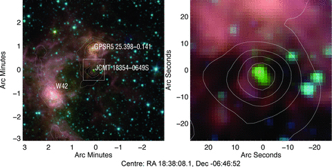
A colour composite image of IRAC photometric bands where red is IRAC 8.0 μm, green is 4.5 μm and blue is 3.6 μm. Images are logarithmically scaled and combined into one composite image. The area enclosed in a white rectangle is the target source JCMT I18354−0649S and the image on the right is a close-up of this region. GPSR5 25.398−0.141 and W42 are nearby UCHii regions. In both images, contours are from 850 μm continuum JCMT SCUBA data. The contours start at 3σ and increase by 1σ thereafter. The position of each object and the scale are indicated on the image.
Sub-millimetre continuum SCUBA pipeline reduced and calibrated mosaics at 450 μm and 850 μm were acquired from the JCMT archive.1 The observations were taken in 2003 September using a 64-point jiggle pattern to ensure sufficient coverage of the sky. The sky opacity was estimated from skydip observations giving an average τ850 of 0.3 and τ450 of 1.6 and observations of Uranus taken on the same night in the photometry mode were used to derive flux calibration factors (FCF) of 244 Jy V−1 and 344 Jy V−1 for the 850 μm and 450 μm maps, respectively.
Fig. 1 shows a colour composite view of the region constructed from Spitzer IRAC images. The overlaid contours from 850 μm JCMT SCUBA data highlight the structure and the extent of the dust emission in the area. JCMT 18354S is situated in close proximity to the prominent Ultra Compact H ii (UCH ii) region GPSR5 25.398−0.141 to the north and W42 to the south-east. Wu et al. (2005) report that JCMT 18354S is only detectable in sub-millimetre and millimetre wavelengths and suggest that this is indicative of its early stage of evolution. However, close examination of Fig. 1 reveals an object visible in all IRAC broad-bands at the very same position as the sub-millimetre core (this data may have been unavailable to Wu et al. 2005). The new feature detected only in Spitzer IRAC bands is strongest in 4.5 μm and could well indicate emission originating from numerous H2 lines present in those wavelengths (Smith & Rosen 2005; Ybarra & Lada 2009) which would make JCMT 18354S a so-called green fuzzy object (Chambers et al. 2009). IRS spectra will be required to confirm the nature of the shocked feature.
Molecular line observations of JCMT 18534S were obtained in 2007 August and 2008 April with the JCMT using the RxA receiver operating from 211 to 279 GHz frequencies and Auto-Correlation Spectrometer and Imaging System (ACSIS) autocorrelator system in a position switching mode. The average full width at half max of the JCMT beam is 20 arcsec, and our obeservations are Nyquist sampled at 10 arcsec with a main beam efficiency of 0.69. We followed the strategy described in Wu et al. (2005) during their 2004 observing campaign (listed in Table 1) choosing the same reference OFF-position (800 arcsec, 800 arcsec) since it was free of emission at the frequencies observed (HCN, HCO+, H13CO). Telescope pointing was regularly checked using the UCHii region GPSR5 25.398−0.14 situated to the North.
Our observations were supplemented with JCMT archive data of the JCMT 18534S taken with the RxA and RxB (325–375 GHz) receivers and DAS autocorrelator. In all cases, the same type of position-switching mode was implied apart from the 12CO (J= 3–2) line where the raster-mapping mode was utilized. The typical system temperatures (Tsys) for RxA and RxB receivers are about 200 K and 600 K, respectively. All the archival data were reduced using the specx package incorporated in the starlink suite. Data taken with the new ACSIS autocorrelator were processed using tasks in packages smurf and kappa from the starlink suite.
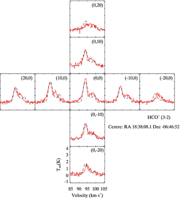
Additional spectral line data were obtained in 2008 July with the Mopra Telescope, operated by the Australia Telescope National Facility (ATNF). The observations were taken with the Mopra Spectrometer (MOPS) in a zoom mode to obtain on-the-fly (OTF) maps. Each 3 × 3 arcmin OTF map took 30 min to cover, and pointing checks on SiO maser sources were carried out every hour. Several OTF maps were made at each tuning to improve the signal-to-noise ratio by increasing the integration time. To reduce the effect of scanning artefacts, the telescope alternated between scanning in right ascension and declination. The data were reduced with the livedata and gridzilla packages (Barnes et al. 2001), which corrects the bandpass for the of-source reference spectra and fits a polynomial baseline to the data. miriad was used to smooth the spectra from the original 0.1 km s−1 pixels, by a seven-point Hanning function, to improve the signal-to-noise ratio, and resampled to 0.2 km s−1 pixels (Nyquist sampled). The beam size, Tsys and efficiency of the Mopra Telescope are 36 arcsec, 200 K and 0.49 at 86 GHz and 33 arcsec, 600 K and 0.42 at 115 GHz (Ladd et al. 2005). All spectra presented in Figs 4–16 indicate their position as an offset from the same common centre which is centred on the 850 μm emission peak of JCMT 18534S at  . In all cases, the mapping offset positions are indicated in the individual figures.
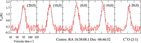
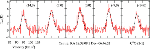
C17O (2–1) line spectra taken with the JCMT. The frequency of this transition is 224.71 GHz and the spectral resolution is 0.24 km s−1. The line profile positions are with respect to the centre of Fig. 1 and each line profile is offset from each other by 10 arcsec. The red solid line is the data and the black dashed line is the model.
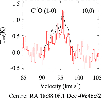
C17O (J= 1–0) line spectra taken with the Mopra Telescope. The frequency of this transition is 112.36 GHz and the spectral resolution is 0.18 km s−1. The line profile positions are with respect to the centre of Fig. 1. The red solid line is the data and the black dashed line is the model.
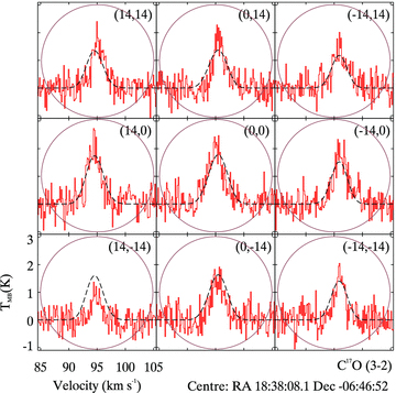
C17O (3–2) line spectra taken with the JCMT. The frequency of this transition is 337.06 GHz and the spectral resolution is 0.14 km s−1. The line profile positions correspond to the centre of Fig. 1 and each line profile is offset from each other by 14 arcsec. The circles show the pointing pattern used in this transition only since it is undersampled with respect to the JCMT beam.
C18O (J= 2–1) line spectra taken with the JCMT. The frequency of this transition is 219.56 GHz and the spectral resolution is 0.24 km s−1. The line profile positions correspond to the centre of Fig. 1 and each line profile is offset from each other by 7 arcsec.
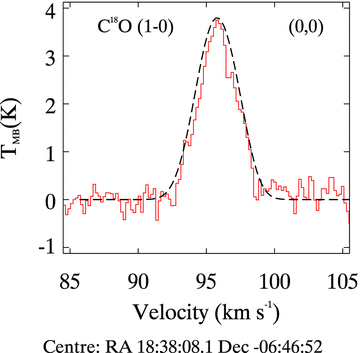
C18O (1–0) line spectra taken with the Mopra Telescope. The frequency of this transition is 109.78 GHz and the spectral resolution is 0.18 km s−1. The line profile position corresponds to the centre of Fig. 1.
HCO+ (J= 1–0) line spectra taken with the Mopra Telescope. The frequency of this transition is 89.19 GHz and the spectral resolution is 0.23 km s−1. The line profile position corresponds to the centre of Fig. 1.
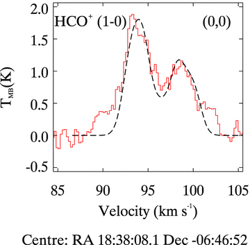
HCO+ (J= 3–2) line spectra taken with the JCMT. The frequency of this transition is 267.55 GHz and the spectral resolution is 0.09 km s−1. The line profile positions correspond to the centre of Fig. 1 and each line profile is offset from each other by 10 arcsec.
H13CO+ (J= 1–0) line spectra taken with the Mopra Telescope. The frequency of this transition is 86.75 GHz and the spectral resolution is 0.23 km s−1. The line profile position corresponds to the centre of Fig. 1.
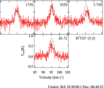
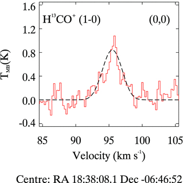
H13CO+ (J= 3–2) line spectra taken with the JCMT. The frequency of this transition is 260.25 GHz and the spectral resolution is 0.09 km s−1. The line profile positions correspond to the centre of Fig. 1 and each line profile is offset from each other by 10 arcsec.
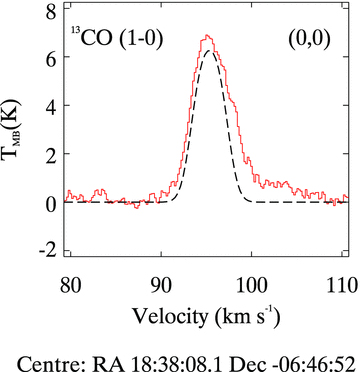
13CO (J= 1–0) line spectra taken with the Mopra Telescope. The frequency of this transition is 110.20 GHz and the spectral resolution is 0.23 km s−1. The line profile position corresponds to the centre of Fig. 1.
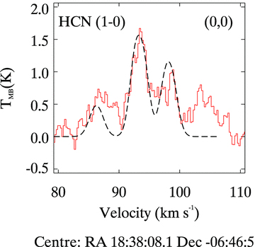
HCN (J= 1–0) line spectra taken with the Mopra Telescope. The frequency of this transition is 88.63 GHz and the spectral resolution is 0.23 km s−1. The line profile position corresponds to the centre of Fig. 1.
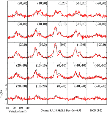
HCN (J= 3–2) line spectra taken with the JCMT. The frequency of this transition is 265.88 GHz and the spectral resolution is 0.21 km s−1. The line profile positions correspond to the centre of Fig. 1 and each line profile is offset from each other by 10 arcsec.
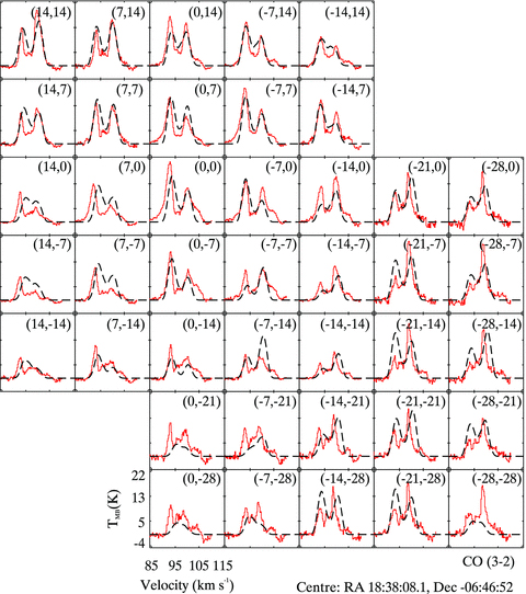
12CO (J= 3–2) line spectra taken with the JCMT. The frequency of this transition is 345.79 GHz and the spectral resolution is 0.27 km s−1. The line profile positions correspond to the centre of Fig. 1 and each line profile is offset from each other by 7 arcsec.
3 MODELLING
In the following sections, a model for JCMT 18534S is carefully developed. First, a semi-analytic depletion analysis is presented in which the degree of freeze-out of molecules on to dust grains is estimated. This is shown to be consistent with the full radiative transfer model which follows. Secondly, the dynamical and radiative transfer model is presented. Many processes (freeze-out, desorption, infall, outflow) occur simultaneously in cold dark molecular clouds. Observed line profiles are made up of emission from gas that is susceptible to many or all of these effects. Different molecular transitions preferentially trace different physical regimes and dynamical phenomena. Including all processes in a consistent model is a difficulty that can be overcome by using a 3D molecular line radiative transfer code. Model fits to observational line profiles are presented in a sequence that allows the dynamical elements of the model to be explained in turn.
The 3D radiative transfer code used throughout this work was written and developed by Keto and collaborators (see e.g. Keto 1990; Keto et al. 2004; Redman et al. 2004; Redman, Keto & Rawlings 2006; Carolan et al. 2008, for examples of its use). The code will shortly be made public under the name mollie (MOLecular LIne Explorer) and is used to generate synthetic line profiles to compare with observed rotational transition lines. In order to calculate the level populations, the statistical equilibrium equations are solved using an Accelerated Lambda Iteration (ALI) algorithm (Rybicki & Hummer 1991) that reduces the radiative transfer equations to a series of linear problems that are solved quickly even under optically thick conditions. mollie splits the overall structure of a cloud into a 3D grid of distinct cells where density, abundance, temperature, velocity and turbulent velocity are defined.
The best-fitting parameters are shown in Table 2 where the number density are in bold font to indicate that it is the peak value of a profile that is shown in Fig. 3. It is created from the observations of SCUBA 850 μm emission with the assumption of spherical symmetry. Initially, the intensity drops off as r−1.5 progressing to a steeper value of r−2. This indicates the presence of a core which is surrounded by a gradually diffuse outer region. The beam size at 850 μm is 14.5 arcsec and the intensity used to derive the density is averaged over the size of the beam.
Parameters for the best-fitting model. The abundance is the ratio of the column density with respect to the column density of H2 or  . The two values of abundance quoted refer to their value inside and outside the freeze-out radius (Section 3.1.4). Included in this table, for comparative purposes, is a list of the best-fitting parameters for the low-mass protostellar core L483. The key feature of this comparison is that gas in cores forming high-mass stars tends to have a higher infall velocity and a much higher turbulent velocity.
| Molecule | Density (cm−3) | Velocity (km s−1) | Temperature (K) | Turbulent Velocity (km s−1) | Abundance (× 10−8) |
| JCMT 18354S (this work) | |||||
| C17O | 106 | 1 | 18 | 1.4 | 0.09 and 0.9 |
| C18O | 106 | 1 | 20 | 1.6 | 0.7 and 8 |
| HCO+ | 106 | 1.5 | 20 | 1.5 | 0.022 |
| H13CO+ | 106 | 1 | 20 | 1.5 | 0.0002 |
| HCN | 106 | 1.5 | 20 | 1.5 | 0.01 |
| 13CO | 106 | 1.5 | 20 | 1.5 | 90 |
| 12CO (envelope) | 106 | 1 | 20 | 1.6 | 1000 |
| 12CO (outflow) | 5 × 10⁴ | 10 | 110 | 1.7 | 6000 |
| L483 (Carolan et al. 2008) | |||||
| C17O | 106 | 0.6 | 10 | 0.1 | 1 |
| C18O | 106 | 0.6 | 10 | 0.1 | 5 |
| 13CO | 106 | 0.6 | 10 | 0.1 | 25 |
| 12CO (envelope) | 106 | 0.6 | 10 | 0.1 | 1700 |
| 12CO (outflow) | 104 | 3.5 | 90 | 1.4 | 3500 |
Parameters for the best-fitting model. The abundance is the ratio of the column density with respect to the column density of H2 or . The two values of abundance quoted refer to their value inside and outside the freeze-out radius (Section 3.1.4). Included in this table, for comparative purposes, is a list of the best-fitting parameters for the low-mass protostellar core L483. The key feature of this comparison is that gas in cores forming high-mass stars tends to have a higher infall velocity and a much higher turbulent velocity.
| Molecule | Density (cm−3) | Velocity (km s−1) | Temperature (K) | Turbulent Velocity (km s−1) | Abundance (× 10−8) |
| JCMT 18354S (this work) | |||||
| C17O | 106 | 1 | 18 | 1.4 | 0.09 and 0.9 |
| C18O | 106 | 1 | 20 | 1.6 | 0.7 and 8 |
| HCO+ | 106 | 1.5 | 20 | 1.5 | 0.022 |
| H13CO+ | 106 | 1 | 20 | 1.5 | 0.0002 |
| HCN | 106 | 1.5 | 20 | 1.5 | 0.01 |
| 13CO | 106 | 1.5 | 20 | 1.5 | 90 |
| 12CO (envelope) | 106 | 1 | 20 | 1.6 | 1000 |
| 12CO (outflow) | 5 × 10⁴ | 10 | 110 | 1.7 | 6000 |
| L483 (Carolan et al. 2008) | |||||
| C17O | 106 | 0.6 | 10 | 0.1 | 1 |
| C18O | 106 | 0.6 | 10 | 0.1 | 5 |
| 13CO | 106 | 0.6 | 10 | 0.1 | 25 |
| 12CO (envelope) | 106 | 0.6 | 10 | 0.1 | 1700 |
| 12CO (outflow) | 104 | 3.5 | 90 | 1.4 | 3500 |
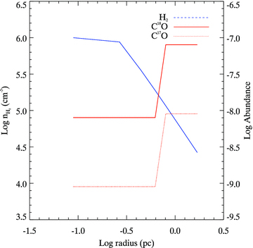
Profiles of the parameters that vary as a function of distance from the centre of the cloud. These profiles show how the H2 density (blue) and molecular abundance (red) vary as a function of distance from the centre of the cloud. The density of H2 varies as a power law and the abundance decreases because of freeze-out.
The velocities in Table 2 are of gas that is moving towards the centre of the core (infall) except for the velocity of 12CO (outflow) whose direction is away from the core centre. The turbulent motion of the gas is characterized with the turbulent velocity parameter. The abundance is the ratio of the column density with respect to the column density of H2 or  .
.
3.1 Freeze-out of molecular gas on to dust grains
While molecular line rotational transitions are a very powerful probe of cloud conditions, continuum observations can also be used to unambiguously investigate some processes. The continuum radiation from dust grains is optically thin in the wavelengths observed in this paper and are used in tandem with molecular line observations to investigate the freeze-out of molecular gas on to dust grains. Freeze-out of molecular gas on to dust grains is expected to occur when the temperature of protostellar clouds is low T≲20 K and density is high  (Sandford & Allamandola 1993). During this phase, it is difficult to observe emission from rotational transitions. However, molecular hydrogen is the dominant constituent of molecular clouds and distinct relationships exist between it and the next most dominant molecule in molecular clouds which is carbon monoxide and its isotopes. With this knowledge, the column density of H2 is inferred from dust and gas emission and a discrepancy between the two indicates that there is significant freeze-out of molecular gas.
3.1.1 Column density from dust emission
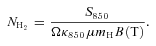
 also in Jy, is calculated assuming a dust temperature of 20 K, mH is the mass of a hydrogen atom in g and μ is the mean molecular weight. A dust mass opacity of κ850= 0.02 cm2 g−1 is assumed which is consistent with Ossenkopf & Henning (1994) and it represents dust grains with thin ice mantles; the dust-to-gas ratio is taken to be 100.
3.1.2 Column density from line emission
 is the integrated intensity of the line profile, S is the line strength, Eu is the energy of the upper level and Q(Tex) is the partition function. An excitation temperature of 20 K is assumed which is consistent with the dust temperature and for C18O and C17O. The partition functions are 7.94 and 7.69, respectively. μ is the dipole moment in Debyes which for C18O is 0.11079 Debye and for C17O it is 0.11034 Debye (Pickett et al. 1998). The conversion factor of C18O → H2 is 2.07 × 10⁶ and C17O → H2 is 7.56 × 10⁶ (Lacy et al. 1994; Wilson & Rood 1994; Ladd, Fuller & Deane 1998).
3.1.3 Column density from a constant abundance model
As a further constraint on the degree of freeze-out, the column density of H2 is determined using mollie. While mollie can implement any type of 3D physical structure, a spherical model is used to approximate the cloud of gas in JCMT 18354S for this calculation only. A constant abundance model is run and from this we have determined the predicted column density of H2 to compare with the column density of H2 calculated from the dust emission. The figures showing the constant abundance model fit to the observed line profiles are not shown in this paper; we only wish to highlight the error of using a constant abundance model.
A best-fitting model was found which matched the peak intensity and width of the line profiles of C18O (2–1), C17O (2–1) and C17O (3–2). The density of H2 has a peak value of 106 cm−3 and varies as r−2 from the centre of the model cloud. This density profile is similar to that observed from low-mass Class 0 protostars by Shirley, Evans & Rawlings (2002). The radius of the core was set at 30 arcsec and is derived from 850 μm emission which is at the 3σ level at this point. This radius is the same as where molecular line emission from high critical density species such as HCN (3–2) and HCO+ (3–2) is just indistinguishable from the continuum. However, there is significant emission observed beyond this radius from gas species with low critical densities.
It was found that an abundance of 1.4 × 10⁻⁸ and 1.0 × 10⁻⁹ for C18O and C17O gave the best fit to the observed line profile. However, these values are an order of magnitude less than estimated using the standard interstellar abundance ratios of H2/CO = 3700, 16O/18O = 560 and 18O/17O = 3.65 (Lacy et al. 1994; Wilson & Rood 1994; Ladd et al. 1998). This result agrees with the outcome of the previous section where the observed integrated intensity gave an H2 column density that is significantly less than that derived from optically thin dust emission.
3.1.4 Comparing the dust and gas emission
The column density of H2 using all three techniques is plotted in Fig. 2 as a function of distance from the centre of the core. There is an order of magnitude difference among the column density of H2 calculated from dust emission, several optically thin molecular gas species and the model. This is caused by freeze-out of molecular gas on to dust grains. To incorporate this effect in mollie, a freeze-out radius is defined. The extent of the freeze-out radius is estimated by comparing the point where the H2 column density derived from dust and gas observations diverges. Referring to Fig. 2, this occurs at ≈20 arcsec (0.5 pc) from the centre of the core. Due to the large beam of the observations, this region is not sampled to a high resolution which creates a sharp drop-off in the abundance, whereas an abundance determined from interferometric observations would show a gradual drop-off.

The column density of H2 was calculated with observations of dust continuum and molecular line emission; in addition, the column density of H2 was calculated from the best-fitting model to the line profiles of C18O (J= 2–1) assuming a constant abundance model. It indicates that significant amounts of the molecular gas are not observed because the gas has frozen out on to dust grains. Therefore, an abundance profile is included in the modelling to account for this effect.
In choosing an abundance and the degree of freeze-out, we are limited by the requirement that the H2 column density derived from gas observations should agree with the H2 column density derived from dust observations. In addition, the modelled and observed spectral line profile should agree. Therefore, the abundance used in our model is the abundance that gives an H2 column density that agrees with the dust-derived column density but which is reduced by an order of magnitude inside the freeze-out radius.
3.2 Gas dynamics
In this section, the inclusion of several global dynamical processes in the model for JCMT 18354S is justified. The molecular line transition that best exhibits each process is shown together with the model fit. It should be emphasized that the model line profiles are from the final overall model and that some transitions are affected by several of the effects discussed below. The model parameters are displayed in Table 2 and discussed in Section 4.
3.2.1 Rotating molecular gas
The line emission spectra of three transitions in C17O are shown in Figs 4–6. Alongside the observed line profiles (red) are line emission profiles from the best-fitting model (black) created using mollie. The line profiles are created using a model where the abundance varies due to freeze-out as discussed in the previous subsection. Fig. 3 shows the abundance and density profile used to model the transitions of C17O and C18O. The temperature and velocity of the turbulent gas are kept constant throughout the cloud in this model. The position of the peak intensity shifts in position on the velocity axis. This shift is most readily seen in the C17O (Figs 4–6) and C18O (Figs 7 and 8) transitions. These lines show a shift in the position of the peak intensity which is caused by rotating gas. It is found that a rotational velocity of 0.5 km s−1 in the model gives the best fit to the observed line profile.
3.2.2 Turbulent molecular gas
Two rotational transitions of the C18O molecule are shown in Figs 7 and 8. The line emission profiles are single peaked and very broad (∼3 km s−1) with respect to line emission profiles of the same transition from low-mass protostellar cores (Carolan et al. 2008). The best-fitting model to the observed line profile includes gas with a high turbulent velocity ≈1.5 km s−1. This parameter is constrained from a comparison of the modelled line emission profile and the hyperfine line emission in the three transitions of C17O. The hyperfine lines are readily observed in low turbulent velocity gas from low-mass protostellar cores (Redman et al. 2002). Figs 4–6 are actually composed of hyperfine lines but instead they are blended together indicating that the gas is highly turbulent.
3.2.3 Infalling molecular gas
The detection of infalling molecular gas is one of the key indicators of star-forming activity in low-mass protostellar clouds. The envelope acts a reservoir for new material and the radius within which gas is infalling grows with time. Optically thick emission from gas creates its own distinctive line profile. The ‘classic’ signature of the infalling gas is a blue asymmetric line profile where the blueshifted emission peaks at a higher intensity than the redshifted emission (Myers et al. 1996). The asymmetry occurs because radiation from warm gas at the centre of the cloud is absorbed by cooler gas that lies farther out. In contrast, the blueshifted emission does not pass in front of an absorbing layer of gas thereby creating an asymmetric line profile.
HCO+ and H13C O+ were used to trace infalling molecular gas. Figs 9 and 10 show the line emissions of two different rotational transitions from the HCO+ molecule. Both line profiles show a clear blue asymmetric line shape which is characteristic of the infalling gas. The lines are fitted with a model that includes infalling gas with a velocity of 1.5 km s−1. Two rotational transitions of H13CO+ are shown in Figs 11 and 12, respectively. The line profiles are single peaked though there may be a slight shoulder in the spectra of the (1–0) transition as the opacity of the radiation is higher in the lower transitions. In contrast to HCO+, the signature of the infalling gas is not seen in the line emission from H13CO+ because it is not as abundant enough that the optical thickness can get very high. Single-peaked H13CO+ lines also effectively rule out the possibility that the double-peaked HCO+ profiles could be caused by two cores.
Figs 11 and 12 are optically thin transitions that peak in intensity at the same velocity as the (J= 1– 0) and (J= 2–1) transitions of C18O and the (J= 1– 0), (J= 2–1) and (J= 3–2) transitions of C17O. The H13CO+ molecule has an abundance significantly less than HCO+ which affects the observed line profile in two ways. First even though it is tracing infalling gas there is no self-absorption and therefore a double-peaked, blue asymmetric spectral line is not observed. Secondly, the spectral line is predominately Gaussian and peaks at the systemic velocity of the molecular cloud.
The velocity at which optically thin gas peaks in intensity (see Fig. 12) should coincide with an absorption dip in line profiles from infalling optically thick gas. In Figs 9 and 12, such a characteristic line profile is seen suggesting that these lines are greatly effected by the infalling gas. In both species, the infall velocity of the gas is constant as a function of distance from the centre of the cloud but a velocity shift similar to that detected in the optically thin CO species (Section 3.1) of 0.5 km s−1 is also seen in these line profiles.
The line emission spectra from the (J= 1– 0) rotational transition of 13CO are shown in Fig. 13. The critical density of this transition is three orders of magnitude less than both the HCO+ and H13CO+ lines and the peak density of molecular hydrogen in this cloud. Therefore, the emission that is observed originates from a different dynamical region than HCO+ or H13CO+. The line shape in Fig. 13 has a slight blue asymmetry which indicates infalling gas. The asymmetry is not too severe and there is no double-peaked line shape which indicates that this line is tracing the slowest infalling gas that resides at the outmost edge of the infall region.
3.2.4 HCN as a dynamical tracer?
The HCN line profiles are shown in Figs 14 and 15 and show the (J= 1–0) and (J= 3–2) rotational transitions. The critical densities ncrit of these transitions are 2.6 × 10⁶ and 5.2 × 107 cm−3 which are both higher than the peak density of molecular hydrogen in our model ( ).
).
When the density is larger than ncrit, an excited molecule will transfer its energy to a collision partner such as H2 and He before it has time to emit the radiation as a photon. This collisional de-excitation is important for low critical density species such as CO; however, the HCN lines shown in Figs 14 and 15 arise from gas that is dominated by radiative de-excitation. This means the rotational transitions that are observed here probe the gas in the dense core. The (J= 1–0) line profile may be effected to some extent by collisional de-excitation as its critical density is close to the peak density of molecular hydrogen.
The HCN emission profile contains hyperfine line emission which complicates the observed line profile. This is unfortunate for using HCN as a gas dynamical tracer species for distant massive star-forming regions because it does have other features, such as a large critical density, that make it an ideal physical probe. The drawback is the hyperfine structure of the rotational lines due to the nuclear quadrupole moment of 14N. At the low J levels, the hyperfine components are well separated and at higher J levels they are blended. The HCN (J= 1– 0) line, for example, has hyperfine components spread over ∼13 km s−1. A further complication, beyond the scope of this work, is that HCN often exhibits poorly understood ‘hyperfine anomalies’ where the individual hyperfine components are boosted or suppressed far beyond what would be expected if they are in thermal equilibrium with each other (Guilloteau & Baudry 1981; Bains, Cunningham & Lo 2009).
The hyperfine structure is just resolved in our HCN (J= 1–0) observations. It is not clear whether hyperfine anomalies are present in these line data because the dynamics of the source plus the usual opacity effects along the line of sight lead to a highly confused line profile shape and somewhat poor model fit. While the hyperfine structure is not resolved at HCN (J= 3–2), its underlying effects are apparent in the larger observed line splitting due to infall of HCN (J= 3–2) than HCO+ (J= 3–2).
In general, it is a mistake to select HCN (J= 3–2) as an infall tracer for quantitative work simply on the basis that the line splitting is sharper since in fact this is due to the underlying hyperfine structure. In addition, the possible presence of poorly understood HCN hyperfine anomalies means that this molecule must be used with great caution as a dynamical tracer. This point is being developed by Redman et al. (in preparation).
3.2.5 Molecular outflow
Jet-driven molecular outflows are detected alongside cores forming massive stars (Shepherd & Churchwell 1996; Shepherd 2005), low-mass stars (Lada 1985; Fukui 1989; Reipurth & Bally 2001; Cabrit 2003) and brown dwarfs (Whelan et al. 2007; Phan-Bao et al. 2008; Whelan, Ray & Bacciotti 2009) which suggests that they are ubiquitous to the star formation process. Their role is to remove angular momentum in the core that results from spin-up due to accreting gas. Outflowing gas tends to have broad wings of emission indicating gas at a high velocity with respect to the systemic velocity of the core. The optically thick lines 12CO often have two distinct peaks of emission separated in velocity by a few km s−1. This is readily seen in observed line emission profiles of the lower rotational transitions.
Fig. 16 shows the CO (J= 3–2) rotational transition line emission over a 50 arcsec × 50 arcsec area. The lines profiles are clearly double peaked and asymmetric. The asymmetry of the line shape switches from blue asymmetric at (0,0) to red asymmetric at (−21,−14). Such switches in peaks of intensity are also seen in the outflow lobes in low-mass star formation. The observed line profiles were fitted with a model that includes all the physical parameters constrained from the observations presented earlier. 12CO is the second most abundant molecule in molecular clouds. This makes it a good candidate for tracing the molecular outflow since an outflow occupies a small fraction of the volume of a cloud. Our best-fitting model indicates that the emission is coming from a bipolar structure. The orientation of the outflow with respect to the line of sight creates the double peaks of the spectra in Fig. 16. The double peaks represent emission that is blueshifted and redshifted because the outflowing gas is pointed towards and away from the observer, respectively (Rawlings, Redman, Keto & Williams 2004). The asymmetry in the intensity changes with the orientation of the outflow axis to the line of sight. An angle of 30○→ 40° for the outflow axis to the line of sight gave the best fit to the observed line profiles. It should be noted that the peak of 12CO (J= 3–2) emission coincides with the peak of the dust continuum emission as seen in Fig. 1. This effect is due to a combination of the orientation of the outflow axis to the line of sight and the large beam size of the line emission observations. A schematic of the structure of JCMT 18354S is given in Fig. 17, and it indicates how the orientation of the outflow axis will result in the gas from the outflow lobes coinciding in the line of sight with the centre of the cloud.
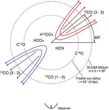
A schematic representation of the regions in JCMT 18354S that are traced by each molecular line. The orientation of the outflow in the plane of the sky and the lobes of redshifted and blueshifted emissions are indicated with different colours.
The 12CO line profiles are better fitted in the outlying regions rather than in the centre of the core. This is caused by a rapidly changing temperature and morphology in the centre. In contrast, the gas that is farther out in the lobes of the outflow comes from a region where conditions are much more stable. The result is that gas originating in the lobes is easier to model whereas in the centre where the gas is changing rapidly and localized in a small region, it is more difficult.
The presence of outflowing gas is a good indicator of star formation activity in low-mass protostellar cores and the modelling here demonstrates the major effect on the 12CO (J= 3–2) line emission observed in JCMT 18354S. The blueshifted outflow emission coincides with the peak in emission of the IRAC image in Fig. 1. There is no IRAC emission on the redshifted side because it is obscured by dense gas in the line of sight. In addition, archival SiO (J= 6–5) and (J= 2–1) emission line profiles (which are not displayed or modelled, since SiO is not yet fully incorporated into mollie) peak at the same location as the IRAC emission. SiO emission normally indicates recently shocked gas and in low-mass cores, it is shown to trace the molecular outflow (Santiago-Garcia et al. 2008). We therefore consider the SiO and IRAC emission to be tracing the molecular outflow.
4 DISCUSSION
The model described in the previous section is of a massive protostellar core undergoing infall, outflow, rotation and depletion. The best-fitting physical parameters for each molecular species for the model are shown in Table 2. Further improvement to the fits, particularly the outflow wing line profiles, may be obtained by introducing a gradient in the turbulent velocity, allowing for a velocity structure within the outflow and incorporating a chemical model to allow for more realistic variations in the species abundances.
In order to compare the properties of JCMT 18354S to those prevalent in low-mass star formation, the results of a modelling exercise for a typical nearby low-mass star-forming core, L483 (Carolan et al. 2008), are also presented in Table 2. The central density and radius (and thus overall mass) of the cold massive core are higher as would be expected. However, many of the parameters are strikingly similar between the two cores. The physical properties of the cloud gas such as the temperature, degree of depletion and molecular abundances of the low- and high-mass cores are comparable. The global behaviour of the massive star-forming system is also similar to that of low-mass star formation: infall, rotation and outflow are all implied by the observations and modelling. These dynamical processes act on larger physical scales and support the interpretation of massive star formation as a scaled-up version of low-mass star formation, at least at this evolutionary stage.
The most significant differences between the two classes of object are in the infall and turbulent velocities, both of which are an order of magnitude greater than gas in low-mass cores. This difference is very significant because in cold massive cores, such velocities are highly supersonic compared to the isothermal sound speeds. The large velocity in both the infalling and turbulent gas is ultimately due to the large gravitational potential well at the centre of the molecular cloud. The dynamics of the cold massive core are thus dominated by supersonic velocities.
The supersonic turbulence could be interpreted literally as just that: very energetic turbulence in one large gas cloud. Supersonic turbulence will undergo collisions of gas streams and the formation of localized eddies. Shocks must result since the motions are highly supersonic which will lead to localized dissipation of energy and then may lead to the formation of dense clumps. These clumps may either become self-gravitating or more transient structures that then quickly dissipate (Garrod et al. 2005). The observations presented here do not have the spatial resolution to resolve the small-scale structure to test the clumpy cloud scenario discussed in Keto & Wood (2006). However, it is possible that clumps existed prior to the collapse of the cloud and that the observed supersonic velocities are due to the net effect of individual clumps moving around the gravitational well. It is worth noting that in low-mass star formation, very long-lived gravitationally stable starless cores are observed, that is, in quiescent environments at least, undisturbed clumps can persist without either forming stars or dissipating (Redman et al. 2006). Later in the massive star formation process, such clumps may effect the development of the UCHii region (Redman, Williams & Dyson 1998) but presumably they are the objects that collapse to form the cluster of hundreds or thousands of low-mass stars that form alongside massive stars. A radiative transfer and dynamical model of a clumpy accretion flow will be developed further in future work.
5 CONCLUSIONS
The high-mass protostellar core JCMT 18354S was observed in 16 different molecular line transitions at multiple spatial positions and in dust continuum emission. The presence of the so-called green fuzzy 4.5 μm emission (Chambers et al. 2009), that of the SiO emission and that of broad absorption lines in JCMT 18354S are all consistent with the characteristics of a deeply embedded massive star-forming core (Beuther & Steinacker 2007). However, no 24 μm emission, which would come from warm dust in the vicinity of the protostellar object, is detected.
The entire line data set was self-consistently modelled using mollie, a 3D molecular line transfer code. The large data set tightly constrained the source model to be that of a rotating, depleted, infalling envelope collapsing on to a central protostellar source that has evolved sufficiently to generate a molecular outflow. Comparing these properties to those prevalent in low-mass star-forming core shows very clearly that JCMT 18354S is a scaled-up version of a low-mass star-forming core. The major difference is the highly supersonic internal velocities in this massive core compared to those of low-mass cores. This may lead to the formation of gas clumps which in turn become a population of low-mass stars.
The JCMT Archive project is a collaboration between the Canadian Astronomy Data Centre, Victoria, and the James Clerk Maxwell Telescope, Hilo.
We thank the referee for a prompt and constructive report that led to an improved paper. This research was supported through a Science Foundation Ireland (SFI) Research Frontiers award. PBC received support from the Cosmo-Grid project, funded by the Program for Research in Third Level Institutions under the Irish National Development Plan and with assistance from the European Regional Development Fund. RML was supported by an Irish Research Council for Science Engineering and Technology studentship. We also acknowledge SFI/Higher Education Authority Irish Centre for High-End Computing (ICHEC) for the provision of computational facilities and support.
REFERENCES
Author notes
Based on observations collected at JCMT: The James Clerk Maxwell Telescope is operated by The Joint Astronomy Centre on behalf of the Science and Technology Facilities Council of the United Kingdom, the Netherlands Organisation for Scientific Research and the National Research Council of Canada.
