


Abstract
We present a new maximum likelihood method for the calculation of galaxy luminosity functions (LFs) from multiband photometric surveys without spectroscopic data. The method evaluates the likelihood of a trial LF by directly comparing the predicted distribution of fluxes in a multidimensional photometric space to the observations, and thus does not require the intermediate step of calculating photometric redshifts. We apply this algorithm to ∼27 000 galaxies with mR≤ 25 in MUSYC-ECDFS, with a focus on recovering the LF of field galaxies at z < 1.2. Our deepest LFs reach Mr≈−14 and show that the field galaxy LF deviates from a Schechter function, exhibiting a steep upturn at intermediate magnitudes that is due to galaxies of late spectral types.
1 INTRODUCTION
The galaxy luminosity function (LF) has long been one of the cornerstones of statistical observational cosmology. As the distribution of galaxies as a function of luminosity is closely related both to the halo mass function predicted by structure formation models and to the astrophysical mechanisms governing star formation, the LF provides a fundamental test for models of galaxy formation and evolution. The low-redshift LF has also been extensively studied (see Binggeli, Sandage & Tammann 1988 for a review), and some convergence has been reached on its general shape at the bright end. In the famous parametrization by Schechter (1976), a faint-end power-law slope of α≈−1.2 is the consensus value. The characteristic bright-end absolute magnitude M* is dependent on the magnitude system and filter used, but the determination by Blanton et al. (2003) sets it at M*=−21.18 ± 0.04 in the r band at z= 0.1 (adjusted for H0= 71).
Nevertheless, the LF remains a field of ongoing study as modern instrumentation allows us to survey increasingly fainter galaxies. One aspect that has received great attention is the evolution of the LF with redshift, as this provides a much more stringent test of galaxy evolution models than the single data point that the local LF offers us. Several groups have studied the LF to limits of z≈ 1 (Wolf et al. 2003) or even higher, up to and beyond z≈ 3 (Poli et al. 2003; Giallongo et al. 2005; Marchesini et al. 2007), and have found evidence for evolution. Broadly speaking, early-type galaxies show a marked number density evolution with redshift, while late-type galaxies exhibit a luminosity evolution.
But another frontier in our exploration of the LF lies at low redshifts and very faint absolute magnitudes. Traditionally, the deepest probes of the LF come from studies of galaxy clusters. Providing a sample of hundreds of galaxies at the same distances, clusters offer an opportunity to determine LFs simply by counting galaxies and then applying corrections for sample contamination by unrelated background galaxies. This method has been criticized by Valotto, Moore & Lambas (2001) and shown to potentially produce artificially steepened faint-end slopes for optically selected clusters (Valotto et al. 2004) due to the fact that optical selection favours clusters with a higher-than-average density of background galaxies. However, since it eliminates the need for spectroscopic observations to determine the exact distance of each galaxy, this method has none the less been widely applied and has probed the LF of nearby clusters to spectacular depths (Trentham 1998; Trentham & Hodgkin 2002; Trentham & Tully 2002). Frequently, LFs calculated in this way show an upturn in the LF, setting in several magnitudes below the characteristic bright-end magnitude M*, from a slope of α≈−1.2 to a much steeper slope of α≈−1.5. More recently, a similar upturn has also been claimed by Popesso et al. (2005) based on applying the background subtraction technique to clusters in the SDSS. However, for a sample of clusters at z≈ 0.3, this has also recently been debated by Harsono & de Propris (2008), who are also working with statistical background subtraction, but find no evidence for an upturn in the cluster LF. Furthermore, Rines & Geller (2008), working with a spectroscopic sample, find that the LFs of the Virgo Cluster and Abell 2199 can be represented by single Schechter functions consistent with the canonical values of α in the range of −1.1 to −1.3, and attribute the discrepancy from other studies to the use of statistical background subtraction without spectroscopic membership confirmation in the earlier work. In principle, an upturn is not implausible. It is known that galaxies with different morphologies or spectral types have very different Schechter functions; for example, the LF of late-type galaxies is generally very steep, while that of early-type galaxies is shallower. If both are extrapolated to faint magnitudes and then co-added, a faint-end upturn can be reproduced qualitatively (Wolf et al. 2003), provided that the normalization of the late-type LF is still high enough in these dense environments in order for it to dominate the overall LF at some point. Some surveys of nearby groups and clusters have also reported a ‘dip’ in the LF at intermediate magnitudes (Biviano et al. 1996; Flint, Bolte & Mendes de Oliveira 2003; Mendes de Oliveira, Cypriano & Sodré 2006; Miles, Raychaudhury & Russel 2006), which could also be an indication of a bimodality that would be revealed as the superposition of a shallow and a very steep Schechter function in a sufficiently deep and large survey. However, the fact that spectroscopic surveys of the field or clusters have not yet unambiguously verified this result (because of their generally shallower depth) makes this observation controversial.
It would be extremely important to know if this upturn is real and if it is specific to cluster environments (and thus an indicator of environment-specific processes generating large numbers of dwarf galaxies) or rather a universal feature of the LF. Current cold-dark-matter cosmologies surmise that galaxies are embedded in dark matter haloes, and the low-mass end of the halo mass function is thought to be quite steep, with a power-law slope of α≈−1.8. This is in marked contrast with the LF of field galaxies in the local Universe, which exhibits a fairly flat faint-end slope of α≈−1.2 (Blanton et al. 2001; Norberg et al. 2002). However, the field LF is well established from spectroscopic surveys only to intermediate magnitudes of Mr≈−17. Also, studies of the local LF in the only environment, where we can probe its extreme faint end directly, the Local Group and the nearest of galaxy groups beyond it, prefer a flat faint-end slope all the way down to the extreme dwarf regime of Mr≈−10 (Pritchet & van den Bergh 1999; Flint et al. 2003) or suggest at most a moderately steep slope (Trentham, Sampson & Banerji 2005); these studies, however, suffer from being able to access only a very small cosmic volume. Although new Local Group members continue to be found up to the present day (Simon & Geha 2007), it is unlikely that they will change the census substantially at any but the very faintest luminosities, substantially fainter than the limit at which the steep faint-end upturn in clusters has been claimed to appear. Mechanisms suppressing the formation of galaxies in such low-mass haloes (Koposov et al. 2009) may explain the small number of observable dwarf galaxies at low luminosities, but it is unclear how such mechanisms would account for the presence of a large dwarf galaxy population in clusters.
A tentative suggestion of an upturn in the faint end of the field LF was found by Blanton et al. (2005), who detected a steepening of the slope to α=−1.3 at intermediate luminosities, but speculated that inclusion of low-surface brightness galaxies undetectable by the SDSS might modify this value to α≈−1.5 or even steeper. Apart from this work, the aforementioned studies of the LF in clusters provide the only suggestion of a steeper faint-end slope so far, but these are questionable due to their samples lacking spectroscopic confirmation and therefore being susceptible to background contamination.
The frontier in exploring the LF at higher redshift and to fainter absolute magnitudes therefore lies in pushing the flux sensitivity of samples towards fainter and more distant objects. However, at such low fluxes, spectroscopic redshift determination remains extremely time consuming and has a high failure rate, precluding its application to large samples. As an alternative approach, photometric redshifts are increasingly being substituted for spectroscopic redshifts even in the study of LFs (Benitez 2000; Bolzonella, Pelló & Maccagni 2002). However, it is well known that photometric redshifts are not an equivalent substitute for spectroscopic redshifts; their accuracy is typically of the order of Δz= 0.05(1 +z) even in the best cases, and frequently worse than that, leading to the galaxy distribution being smeared out in luminosity and distance. In addition, they suffer from catastrophic failures; galaxies of very different spectral types and at different redshifts can have similar colours, leading to large errors in their recovered photometric redshift that do not obey Gaussian errors. Even purely Gaussian errors in the photometry therefore inevitably propagate into non-Gaussian errors in the photometric redshift, and samples selected by photometric redshifts are inevitably contaminated by galaxies from galaxy populations outside these selection limits. In addition, the distribution of these errors varies from galaxy to galaxy, depending on its spectral properties, true redshift and magnitude. For all these reasons, the recovered photometric redshifts and, by extension, LFs are always dependent on (explicit or implicit) prior assumptions about the LFs of all galaxy populations at all redshifts – assumptions which, except in the case of very careful analyses, are often neglected or in conflict with the recovered results.
Unfortunately, LF algorithms have adapted only poorly to this situation. The algorithms applied to the problem of recovering LFs from photometric-only samples are based on the same methods used 20 years ago for the recovery of LFs from samples with known spectroscopic redshifts. In the simplest procedure, photometric redshifts are simply substituted for spectroscopic redshifts and, assuming that the errors in the photometric redshifts are sufficiently understood, Monte Carlo simulations can be used to estimate whether a serious bias has been introduced into the recovered LF parameters. This approach can be successful, especially at high redshift, where a given uncertainty Δz in the photometric redshift translates into only a relatively minor uncertainty in the absolute magnitude. An example of a successful application of this procedure to the Multiwavelength Survey by Yale–Chile (‘MUSYC’; Gawiser et al. 2006) (http://www.astro.yale.edu/MUSYC) is found in Marchesini et al. (2007). However, at low redshift, as has been demonstrated in the past (Chen et al. 2003), the problems associated with the redshift uncertainties are generally larger: a redshift uncertainty Δz≈ 0.1, typical for photometric redshift determinations, translates into a significant uncertainty in absolute magnitude. Correspondingly, high-quality multiband photometric data are needed to constrain the redshifts well (Fried et al. 2001; Wolf et al. 2003), but obtaining such extensive data sets is not always practical.
There have been suggestions in the literature for adjustments to the LF calculation that take into account the photometric uncertainties and the resulting uncertainties in the redshift. These have either employed Monte Carlo methods (Bolzonella et al. 2002) or incorporated the photo-z uncertainties analytically into the procedure used for recovering the LF (Chen et al. 2003). However, both methods are based on the idea of evaluating a redshift probability distribution that is centred on the best-fitting recovered photometric redshift, and not centred on the true redshift. The net effect is that the galaxy distribution is subjected to a further convolution with the redshift error function, instead of a deconvolution.
The idea behind the photometric maximum likelihood (PML) method, which we introduce in this paper, is therefore to abandon the concept of assigning individual luminosities and redshifts to individual galaxies, since neither are known in non-spectroscopic surveys. Instead, we constrain the LF by requiring it to reproduce the distribution of galaxies in a parameter space consisting of quantities that are known exactly: the observed fluxes in multiple filter bands. We refer to this parameter space, wherein observer-frame fluxes in multiple filter bands are used as the coordinates, as photometric space. This algorithm achieves a true deconvolution of the observed galaxy distribution into its constituent galaxy LFs, and it allows for a self-consistent solution by avoiding priors that the recovered photometric redshifts and luminosity distributions in photometric surveys normally depend on.
In this paper, we present the first application of the PML to a data set that is an ideal test case for this algorithm, the MUSYC survey (Gawiser et al. 2006). MUSYC is a deep square degree survey (divided into four separate fields), comprising some ∼200 000 galaxies. Photometric data in a multitude of optical and near-infrared (NIR) filter bands exist. For the present study, we use one of the four MUSYC fields, the extended Chandra Deep Field South (E-CDFS), observed in eight filter bands: U, B, V, R, I, z, J and K. The large number of filter bands make this survey very suitable to photometric redshift techniques as well as to the PML. The limiting depth of R > 26 mag means that we can probe the LF to extremely faint limits; the relatively wide area, compared to other pencil-beam surveys, guarantees that even the bright end will still be fairly well sampled at all but the smallest redshifts. With a sample cut at R= 25, the PML permits us to constrain the field galaxy LF to a limit as faint as Mr=−14.
This paper is organized as follows. In Section 2, we briefly discuss the data set, the MUSYC survey. In Section 3, we present our LF algorithm, the PML, and test it using a mock catalogue. In Section 4, we present an application of our method to MUSYC by calculating LF parameters, split up by spectral type, from z≈ 0.05 to z≈ 1.2.
2 DATA
MUSYC is designed to provide a fair sample of the Universe for the study of the formation and evolution of galaxies and their central black holes. The core of the survey is a deep imaging campaign in optical and NIR passbands of four carefully selected 30 arcsec × 30 arcsec fields. MUSYC is one of a few surveys to offer its combination of depth and total area, for additional coverage at X-ray, UV, mid-infrared and far-infrared wavelengths and for providing the UBVRIz′JHK photometry needed for high-quality photometric redshifts over a square degree of sky (availability of NIR data varies from field to field). The primary goal is to study the properties and inter-relations of galaxies at a single epoch corresponding to redshift ∼3, but the favourable combination of depth, area and passband coverage makes it suitable for studies of the general galaxy population over a wide range of redshifts as well as for Galactic astronomy (Altmann et al. 2005).
Imaging data for three of the four MUSYC fields were obtained with Mosaic II on the 4 m Blanco Telescope at the Cerro Tololo Inter-American Observatory (CTIO) in Chile. For the fourth field, the E-CDFS, which we analyse in this paper, our UBVRI imaging results from combining public images taken with the European Southern Observatory (ESO) 2.2 m and Wide-Field Imager by the ESO Deep Public Survey and COMBO-17 teams (Arnouts et al. 2001; Wolf et al. 2004; Erben et al. 2005; Hildebrandt et al. 2005). Our z′ imaging was taken with the CTIO 4 m and Mosaic II. Our JK images of the E-CDFS were obtained with the CTIO 4 m and Infrared Side Port Imager.
Photometric coverage of the four MUSYC fields is not perfectly homogeneous. For the present study, we have thus chosen to focus on one of the four MUSYC fields, namely the E-CDFS, which offers the deepest optical imaging; furthermore, in contrast to the other MUSYC fields at the time of this writing, the optically selected photometric catalogue with UBVRIz photometry has been matched to NIR catalogues in J and K. The large number of spectroscopic redshifts available in the literature also enables us to check the quality of our models by estimating photometric redshifts. This field is centred on RA=03:32:29.0, Dec. =−27:48:47 (J2000).
The data that we use for this analysis are drawn from a catalogue selected by the combined B-, V- and R-band fluxes, and complemented by photometry in the J and K bands. The catalogues of J- and K-band photometric data for the BVR-selected detections have not been published, but separate, K-band-selected catalogues of this field based on the same imaging material comprising the NIR bands are already public and described in Taylor et al. (2009).
The full catalogue of the MUSYC-ECDFS contains 84 410 objects. At the depth of MUSYC, the detections consist primarily of galaxies, but the catalogue also contains point sources [stars and quasi-stellar objects (QSOs)], which we remove based on morphological criteria, using the star/galaxy (S/G) classifier provided by the Source Extractor software (Bertin & Arnouts 1996), which was used in the construction of the detection catalogue. To calibrate the threshold value of S/G, we compare its distribution to the position of a detection in the mR–μR–mR parameter space. In such a parameter space, which is shown in Fig. 1, point sources populate an approximately horizontal band. Experimentally, we find that S/G= 0.97 separates the two populations with minimal overlap. This is demonstrated in Fig. 1 by marking all objects with S/G > 0.97 with asterisks in the left-hand panel and all other objects with dots in the right-hand panel. This is a rather high threshold, compared to values adopted in the literature in similar efforts (i.e. S/G= 0.9, Capak et al. 2003; S/G= 0.7, Rowan-Robinson et al. 2004; S/G= 0.5, Grützbauch et al. 2005), and it is possible that our S/G threshold fails to exclude scattered light from saturated stars or close double star systems. To estimate the impact of the star/galaxy threshold, we have therefore carried out a separate analysis adopting a more conservative threshold of S/G= 0.8 and will compare its results with the default sample where appropriate in Section 4.
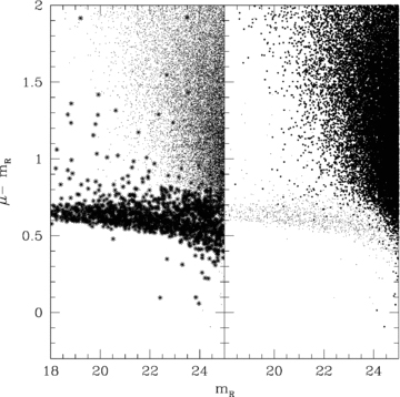
Difference between average surface brightness (in mag arcsec−2) and magnitude mR versus mR. Point sources tend to populate a horizontal branch in this diagram and extended sources an extended cloud on the right-hand side, but the two overlap for faint magnitudes. In the left-hand panel, objects with the star/galaxy class, S/G > 0.97, are marked; in the right-hand panel, objects with S/G < =0.97 are marked. This limit decomposes the two populations with minimal overlap; we therefore accept objects with S/G < =0.97 as galaxies.
For the calculation of the LF from a flux-limited sample, a thorough understanding of the selection function is imperative. The optical MUSYC source catalogues are detected by SExtractor in the combined B-, V- and R-band image, as described in Gawiser et al. (2006). The limiting magnitude for the E-CDFS field is BVR= 27.1 mag (in the AB magnitude system, which is used throughout this paper). For this paper, we apply an additional cut in just a single filter band, the R band, to create our subsample. At R≤ 25 mag, corresponding to a flux limit of R= 0.363 μJy, which is the limit adopted for our analysis, the sample is complete in BVR. Objects with SExtractor warning flags 1, 2 (presence of a close neighbour object possibly affecting the photometry; necessity of deblending) are left in the catalogue; objects with higher warning flags are removed without statistical compensation.
For our analysis, we use ‘corrected aperture magnitudes’ (Gawiser et al. 2006), which yield an estimate of the total flux, but offer a good signal-to-noise ratio (S/N) for compact sources. An exception is very extended objects (with a half-light radius in the BVR image of 1 arcsec or more), for which we substitute the ‘auto’ photometric measurement provided by SExtractor. In addition, we have carried out modifications to the published MUSYC photometry, as described in Appendix A, to adjust the photometric zero points and ensure that the photometric errors conform to a Gaussian distribution. These corrections have significantly improved the quality of the recovered photometric redshifts in comparison to a subsample of galaxies with redshift estimates from the literature, spanning a broad range of redshifts and spectral energy distribution (SED) types, and have brought the uncertainty distribution in line with the assumptions made in our algorithm.
3 METHOD
3.1 Principles of the photometric maximum likelihood approach
The most common type of LF algorithms for magnitude-limited samples of field galaxies is maximum likelihood algorithms. These algorithms are based on the principle of calculating a predicted distribution of galaxies from a trial LF, comparing it to the observed distribution, determining the likelihood of the trial LF and then modifying the latter until the likelihood has been maximized. Traditionally, the distributions that are being compared are the distributions over luminosity (Sandage, Tamman & Yahil 1979; Efstathiou, Ellis & Peterson 1987), sometimes over luminosity plus additional parameters that the LF could depend on, such as spectral type (Bromley et al. 1998; Croton et al. 2005), morphology (Binggeli et al. 1988) or redshift (Poli et al. 2003; Wolf et al. 2003; Giallongo et al. 2005) itself.
In photometric surveys, neither spectral type, nor redshift nor luminosity is known exactly. None the less, past attempts to calculate the galaxy LF from photometric surveys have sought to reconcile the data with the algorithm by simply substituting photometric redshifts for spectroscopic redshifts. This can potentially cause several severe problems as follows.
Random errors in the photometric redshifts ‘blur’ the recovered distances and absolute magnitudes. This introduces systematic biases in the recovered LF, as can be illustrated by a gedankenexperiment. A typical LF is well approximated by a power law at the faint end and has a well-defined exponential downturn at the bright end. If random errors exist in the galaxy redshift, the absolute magnitude estimates of all sample galaxies will be convolved with an error function, which ‘blurs’ the shape of the LF and moves the bright-end ‘knee’ to brighter luminosities. This can be minimized by operating at high redshift (where the impact of redshift uncertainties on the absolute magnitude is smaller) and, of course, with high-quality multiband photometric data.
Systematic errors and catastrophic failures in the photometric redshifts may severely impact the recovered LF. For example, systematic offsets between the photometric redshifts and the true redshift (a common occurrence resulting from errors in the photometric calibration) will directly introduce shifts in the recovered absolute magnitudes. Catastrophic failures (i.e. photometric redshifts significantly and systematically different from the true redshifts) can have a devastating impact; for example, a small number of nearby, bright galaxies mistakenly fitted as high-redshift galaxies may easily dominate the bright end of the LF recovered at high redshift. It is important to note that such catastrophic failures can result simply from the propagation of Gaussian errors of the photometry into the photo-z determination. This means that modelling photometric redshift uncertainties as Gaussians is not legitimate even for perfectly calibrated photometry.
Sample contamination is common. LF determinations are usually carried out for subsamples of galaxies in a confined redshift range and for selected SED types only. However, any subsample selected from photometric redshift data only will almost certainly be contaminated by galaxies at other redshifts and with a wide range of SED types, and incomplete with respect to galaxies that meet the selection criteria [see e.g. Taylor et al. 2009, which argues that photometric redshifts from the COMBO-17 survey (Wolf et al. 2004) suffer from contamination at z > 1 due to the lack of NIR photometry]. Aggravating this problem, the amount of contamination is, of course, dependent on the LF of the contaminant population. Therefore, even if some attempt is made to minimize the contamination (e.g. by introducing an LF prior into the photo-z calculation), the resulting LF is dependent on the LFs of all other galaxy populations at other redshifts.
Various procedures have been suggested for propagating the inherent uncertainties from photometric redshifts into the LF. A simple strategy, proposed by Bolzonella et al. (2002), is to carry out a Monte Carlo simulation, drawing redshifts for each galaxy at random from the probability distribution indicated by the photo-z algorithm. However, the fallacy in this approach is that the Monte Carlo redshifts are drawn from a probability distribution that is centred on the best-fitting photo-z, and not on the true redshift. While this approach does indeed propagate the photo-z uncertainties into the final solution, it does not correct the systematic biases in the photo-z recovery; on the contrary, drawing galaxies from photo-z probability distributions around photo-zs that are already affected by these uncertainties will convolve the solution even more, instead of deconvolving it, and may even exacerbate the systematic errors. A slightly different approach is taken by Chen et al. (2003), who incorporate the photo-z probability distribution into the likelihood function itself. However, inspection of their ansatz shows that the effect is, in fact, again a further convolution of the galaxy distribution, rather than a deconvolution, equivalent to the Monte Carlo approach (it is equivalent to replacing each sample galaxy with a sum of ‘fractional’ galaxies with a range of redshifts); it is thus a more elegant approach suffering from the same problem: the redshift probability distribution is evaluated around a redshift that is not the true redshift.
A mathematically much more consistent method that addresses many of the above criticisms has been suggested more recently by Sheth (2007): the recovered photometric redshift is treated as a quasi-observable distinct from the true redshift, and reproducing its distribution is an additional requirement imposed on the LF algorithm. This approach appears theoretically sound; however, it stops short of replacing the photometric redshift with a different, and easier-to-handle, observable, as we propose here. This raises two practical problems for the application as follows. (1) The algorithm is still based on the concept of a best-fitting photo-z. The procedure of first calculating a best-fitting photo-z and then feeding it as input into an LF algorithm always carries with it a loss of information that is contained in the full photometric vector. (2) The error function of the photometric redshift must be modelled well, which is challenging, as it is a function of many parameters, including the observed flux and true SED of a galaxy. The shape of the photometric redshift probability distribution function varies with the SED, redshift and apparent magnitude of the galaxy in question (e.g. late-type galaxies are much more difficult to constrain than early-type galaxies), and may not even generally be assumed to be Gaussian either, but may in some cases exhibit a complex shape with secondary maxima.
An additional issue that has not been addressed by conventional LF algorithms (but appears to be accounted for by Sheth 2007) is that the probability distribution of photometric redshifts is itself dependent on implicit or explicit prior assumptions about the LF of galaxies at any redshift. Photometric redshifts are therefore dependent on prior assumptions about the redshift distribution of galaxies (i.e. the LF of galaxies of all possible spectral types throughout cosmic history). In photometric redshift determinations, this dependence is often neglected and redshifts are calculated simply as best-fitting estimates, regardless of the redshift or template type that yields the fit. Note, however, that even this approach to photo-z determination carries an implicit and unjustified prior, namely that the prior probability distribution, which depends on the cosmic volume and the LF, is flat with redshift. A more promising approach is Bayesian redshift determination (Benitez 2000), which applies priors (usually in the form of LF priors) to select the most probable photometric redshift. However, while at least the shape of the bright end of the LF is reasonably well known, priors about the faint end and the high-redshift LF are highly uncertain. Furthermore, upon obtaining a new solution for the LF at any redshift, the priors should be modified to accommodate this new information, and the process iterated, so as to avoid a contradiction between the LF result and the assumed prior. If this is not done, a logical inconsistency between the prior applied to the photo-z calculation and the resulting LF will generally result.
In summary, there are four points of criticism that may be raised against the methods employed to recover LFs from photometric samples in the past.
Instead of a deconvolution, they have often carried out a further convolution of the data by applying an assumed error function to the observed data. A proper deconvolution requires that the error function be applied to a model and the resulting distribution be compared to the observed data.
They have evaluated the predicted and observed galaxy distributions in a parameter space consisting of redshift and derived variables, which are not actual observables, but are affected by very complex error functions, which prohibit a direct deconvolution. In such cases, the comparison is more easily carried out in a parameter space consisting of direct observables, allowing us to convolve a predicted data set with the known error function instead.
They have used photometric redshifts and have consequently been forced to evaluate their error functions. Photometric redshifts have very complicated error functions that are usually neither Gaussian nor uniform, but instead feature secondary maxima and are dependent on the magnitude and SED type. But the calculation of LFs does not require knowledge of the redshift of individual galaxies. We therefore suggest to eliminate the photometric redshift from the consideration and focus on direct observables, i.e. the observed fluxes, which have a much simpler error function.
They have often failed to take into account the dependence of the photometric redshift on prior assumptions about the LF at all redshifts. A proper determination of the LF must acknowledge this dependence and ideally provide a self-consistent solution that is not dependent on external priors, but constrained only by the data.
The problems described above arise from the attempt to use established LF algorithms, which were originally developed for samples for which the exact redshifts and, by extension, absolute magnitudes are known, in a context that they were not constructed for, namely, photometric-only galaxy surveys. Our PML method adopts the basic principle of maximum likelihood algorithms: from a trial LF, the galaxy distribution in a certain parameter space (e.g. absolute magnitude) is predicted and the probability for drawing the observed sample from this distribution (i.e. the likelihood of the trial LF) is then calculated. The trial LF is then adjusted to optimize this likelihood. However, the PML algorithm differs from established algorithms by comparing the observed and predicted galaxy distributions in a parameter space consisting only of direct observables, namely the observed photometric fluxes in all available filter bands. We refer to this parameter space as photometric space. This addresses the problems described above.
The PML is able to carry out a proper deconvolution of the observed photometric data. It applies an error function to the expectation values for the photometric fluxes in each filter band and compares the resulting distribution to the observed data.
By evaluating the galaxy distribution as a function of observed fluxes, instead of photometric redshifts, the PML avoids the unnecessary loss of information that is usually incurred when converting the full information of a multiband photometric observation into a single photometric redshift. This also offers the decisive benefit that photometric errors in individual filter bands are much easier to model than those of photometric redshifts.
The algorithm considers the contributions of all LFs at all redshifts to the distribution in photometric space simultaneously, and therefore finds a self-consistent solution for each LF that is (ideally) not dependent on implicit or explicit external luminosity priors.
Our algorithm, by design, naturally accounts for the dependence of the LF on redshift and SED type. An important aspect is the fact that, when evaluating the distribution of galaxies in photometric space, in principle, any galaxy population at any redshift can contribute to the galaxy counts at a given point in photometric space. It is not possible to clearly separate samples by the SED type and redshift. This implies that the likelihood found by the PML algorithm is calculated as a likelihood for all LFs of all galaxy populations throughout cosmic history. This appears at first as a drawback, greatly enlarging the number of free parameters involved in the problem. However, as has been pointed out above, in the conventional approach, it is not strictly possible to clearly separate a sample by redshift and SED type either. Any association of an individual galaxy with a given redshift and SED type is only a statistical one, and under proper Bayesian consideration, the probability for any such association is dependent on the prior assumptions about the LFs of all galaxy populations that a galaxy could in principle have been drawn from. Whereas this dependence usually goes unacknowledged, it is made explicit in the PML, and the problem of introducing external priors is (in an ideal case) eliminated by solving for all contributing LFs simultaneously.
3.2 Derivation
The derivation of a maximum likelihood algorithm starts with the definition of the likelihood function, i.e. the probability that the observed data of a galaxy survey would have been obtained from a given trial LF. The specific likelihood function that we use is inspired by the approach of Marshall et al. (1983), which has also been used more recently by Poli et al. (2003) and Giallongo et al. (2005) for the determination of galaxy LFs, which uses a product of Poisson probabilities of deriving the survey probability.
Here, λ(fi) df is the expectation value of the number of galaxies in cell [fi;df] of photometric space. The index i runs over all observed galaxies, while the index j runs over all cells of flux space that are not occupied by a galaxy. In contrast to Marshall et al. (1983), Poli et al. (2003) and Giallongo et al. (2005), we apply this likelihood evaluation to the distribution of galaxies in photometric space, while the previous work makes use of the availability of full or partial spectroscopic coverage to evaluate the galaxy distribution as a function of luminosity and redshift. This distinction is the defining feature of the PML.
Recently, Kelly, Fan & Vestergaard (2008) have suggested that the proper statistical distribution to use is a binomial one, rather than the Poisson distribution used in the ansatz of Marshall et al. However, they acknowledge that, for surveys that sample only a small fraction of the total sky, which is certainly the case for MUSYC, Poisson distributions are acceptable.
In our sample, we do not have the luxury of spectroscopic redshifts. It is therefore necessary to introduce a mapping between the LF parameters and photometric space. We assume that the photometric data points are distributed according to a Gaussian distribution centred on the expectation value for a given absolute magnitude  and redshift z0 and, furthermore, that the photometric errors are independent in each filter.
 – and evaluates their contributions to the galaxy density in photometric space at the flux position fi. The term
  is the differential comoving volume and P is the assumed parameters of the LF whose likelihood we wish to test. The fraction of galaxies with the physical parameters
  and z0 that contribute to the galaxy density at a point fi is determined via the probability term pσ– the χ2 probability density resulting from a comparison between the fluxes predicted for these parameters and the observed fluxes; this distribution is used here under the assumption that the errors in each filter band are uncorrelated with each other and that the photometric uncertainties in each band are Gaussian. This probability term is our assumed photometric error function. The denominator is the product of the observed flux uncertainties and serves to normalize the probability distribution. We use the following definition of the dimensionless probability density:
We use the empirical measurement uncertainties Δfid of galaxy i to define the χ2 statistic. This is a compromise. A more consistent approach would be to select uncertainties appropriate for the predicted fluxes of the galaxy in each filter band. However, this would require an error model reproducing accurate uncertainties in every filter band as a function of flux. As the photometric uncertainties are largely dictated by conditions other than luminosity alone (such as the surface area of the galaxy), this would require additional assumptions that would weaken, rather than strengthen, our case. We believe that the substitution of the empirical uncertainties in this definition is a justifiable compromise.
A notable point about this approach is that the absolute magnitude of an individual galaxy enters via the normalization of the SED in any desired rest-frame filter band (which need not be identical to the filters used in the survey). The k-correction is therefore integrated into the algorithm implicitly, and the absolute magnitude for a given galaxy at a given redshift and SED is constrained by all available filter bands, rather than by a single band and a corresponding k-correction; it is therefore usually quite precisely constrained. A caveat is that the accuracy of absolute magnitudes depends on the accuracy of the templates; therefore, although the algorithm is in principle capable of calculating LFs in any desired rest-frame filter band, it is desirable that the luminosity in this filter band be well constrained by the available photometry (i.e. we would distrust rest-frame LFs in filter bands at the extreme red or blue end of the survey coverage).
As equation (2) shows, the PML accounts intrinsically for the dependence of the LF on redshift, spectral type and, if desired, other parameters of the LF. It also automatically accounts for the effect of photometric uncertainties on the recovered LF. Most importantly, however, it combines the functionality of a photometric redshift algorithm with that of an LF algorithm via the probability term  , which relates a given galaxy population to the galaxy distribution in photometric space.


Here, the first term represents the likelihood of drawing the observed galaxies from the assumed input LFs, while the second term is simply the total predicted number of galaxies within the flux limits of the survey. The expression df, the volume of one of our cells in photometric space, can be omitted, as it will only add a constant offset of S. Increasing the assumed space density of any galaxy population (e.g. by increasing the normalization of the LF) will decrease the first term, reflecting the greater probability of drawing the observed galaxies from such an input LF, but it will also increase the second term, the total number of galaxies expected in the survey. The LF that balances these terms by minimizing the function S is the maximum likelihood LF.
Calculating λ(f) in the second term requires an assumption regarding the width of the distribution, i.e. the photometric errors of a hypothetical galaxy at a point f in the photometric space, in order to correctly represent the contributions of galaxy populations near the flux limit of the sample to the total number of observed galaxies. It should be set to a value typical of the survey under consideration; we have experimentally found that the impact of this value on the recovered LFs is very minor. We set it to 25 per cent of the flux, which is characteristic of most objects near this flux limit. This value determines the fraction of galaxies whose observed fluxes scatter across the survey limit, and it will influence the solution only if the faint end of the LF is very steep, i.e. if a much larger number of normally unobservable galaxies scatter above the survey limits due to photometric errors than vice versa.
Despite our magnitude threshold of R≤ 25, there are galaxies in the catalogue that are consistent with the zero flux in at least one other filter band. As a result, the algorithm may associate them with extremely faint populations that would normally not be expected to contribute to galaxy counts at all, given our model SEDs and the nominal flux error of 25 per cent. Inclusion of such objects may prevent a full convergence of the LF solution, especially in parameters that are constrained by a few other objects. To prevent this, we only evaluate contributions to λi from populations that yield a non-zero contribution to the total expectation value for the number of galaxies in the survey. In other words, we ignore potential contributions to the observed galaxy sample from populations that should, assuming reasonable SEDs and photometric errors, be outside the survey flux limits anyway.
The fact that no precise redshift information is available does imply that the PML shares a disadvantage with the traditional  method: it requires certain assumptions about spatial homogeneity of the LF, violation of which may bias the results. In a non-spectroscopic sample, this is generally unavoidable, because photometric redshift uncertainties wipe out detailed information about a large-scale structure. To the extent that the photometric information permits it, the PML may constrain the LF in several independent redshift bins and thus reproduce gross features of the cosmic galaxy density fluctuation.
3.3 Parametrization of the luminosity function


This equation is derived from equation (9) simply by substituting M* with a redshift-dependent M*(z) =M*0−δlog 10[(1 +z)/(1 +z0)]. Here, M*0 is the characteristic bright-end magnitude evaluated at a fiducial redshift z0. To minimize covariances between M*0 and δ, z0 should be chosen as the redshift at which M* is best constrained by the sample. In our case, we have experimentally found that, for both early- and late-type galaxies, the M*0–δ covariance is minimized for z0≈ 0.95.
For modelling the LF as a function of the SED type and redshift, we assume that each SED template type is described by a Schechter function with a constant α, M* and δ. As photometric data cannot resolve density fluctuation on arbitrarily small scales, we assume that the LF for a given SED type is constant in each of 10 redshift bins that we divide the redshift range 0.02 ≤z < 6 into. Potential density fluctuations on scales similar to or larger than these bins can therefore be reproduced by the algorithm. The redshift bins, along with the approximate limiting absolute magnitudes for early- and late-type galaxies, are shown in Table 1. The divisions between redshift bins are motivated by the desire to apportion approximately equal numbers of observed galaxies to each bin. Also, we have attempted to reflect the robustness of photometric redshift constraints in the choice of binning. Although this model represents a compromise, the number of free parameters is still considerable.
Redshift bins.
| Bin | z |  |  |
| 1 | 0.02 – 0.1 | −11.5 | −11.5 |
| 2 | 0.1 – 0.25 | −14 | −14 |
| 3 | 0.25 – 0.4 | −15.75 | −15.5 |
| 4 | 0.4 – 0.6 | −17 | −16.5 |
| 5 | 0.6 – 0.8 | −18.5 | −17.75 |
| 6 | 0.8 – 1.2 | −20 | −19 |
| 7 | 1.2 – 1.5 | −21.5 | −20 |
| 8 | 1.5 – 2.5 | −22.75 | −20.75 |
| 9 | 2.5 – 3.5 | −23.75 | −21.75 |
| 10 | 3.5 – 6.0 | −24.5 | −22.75 |
| Bin | z | | |
| 1 | 0.02 – 0.1 | −11.5 | −11.5 |
| 2 | 0.1 – 0.25 | −14 | −14 |
| 3 | 0.25 – 0.4 | −15.75 | −15.5 |
| 4 | 0.4 – 0.6 | −17 | −16.5 |
| 5 | 0.6 – 0.8 | −18.5 | −17.75 |
| 6 | 0.8 – 1.2 | −20 | −19 |
| 7 | 1.2 – 1.5 | −21.5 | −20 |
| 8 | 1.5 – 2.5 | −22.75 | −20.75 |
| 9 | 2.5 – 3.5 | −23.75 | −21.75 |
| 10 | 3.5 – 6.0 | −24.5 | −22.75 |
Broad redshift bins within which we analyse the LF. Mearlylim and Mlatelim give approximate effective magnitude limits around which the completeness of our sample drops below ∼10 per cent for average early- and late-type SEDs, respectively.
Redshift bins.
| Bin | z | | |
| 1 | 0.02 – 0.1 | −11.5 | −11.5 |
| 2 | 0.1 – 0.25 | −14 | −14 |
| 3 | 0.25 – 0.4 | −15.75 | −15.5 |
| 4 | 0.4 – 0.6 | −17 | −16.5 |
| 5 | 0.6 – 0.8 | −18.5 | −17.75 |
| 6 | 0.8 – 1.2 | −20 | −19 |
| 7 | 1.2 – 1.5 | −21.5 | −20 |
| 8 | 1.5 – 2.5 | −22.75 | −20.75 |
| 9 | 2.5 – 3.5 | −23.75 | −21.75 |
| 10 | 3.5 – 6.0 | −24.5 | −22.75 |
Broad redshift bins within which we analyse the LF. Mearlylim and Mlatelim give approximate effective magnitude limits around which the completeness of our sample drops below ∼10 per cent for average early- and late-type SEDs, respectively.
3.4 Error calculation
 for every set of trial LF parameters. Therefore, in principle, uncertainty contours on any parameter can be determined with the method of Avni (1976), i.e. the uncertainties are given by the set of parameter values of a constant likelihood
Here,  is the maximum likelihood and Δχ2 is the χ2 value for the desired level of confidence and the appropriate number of degrees of freedom. The latter is usually the number of parameters whose uncertainties we are examining, i.e. two if we are considering the uncertainties in the M*–Φ* plane. Following the example of Avni, we call these parameters the ‘interesting parameters’, while referring to all other parameters that the likelihood may or may not depend on, but whose values do not interest us at the moment, as the ‘uninteresting parameters’. Equation (13) requires that, for any choice of interesting parameters whose likelihood we wish to probe in order to find their uncertainty contours, the likelihood be maximized with respect to all uninteresting parameters.
There are some parameters in our model for the LF and its evolution that we include neither in the best-fitting search nor in the uncertainty calculation; we refer to these as background parameters. In our case, we treat the LF parameters of the very high-redshift and very low-redshift LFs, which are ill-constrained by our data and sensitive to systematic errors, as such background parameters. We set these to realistic values motivated by extrapolating the α, M* and Φ* values from the constrained redshift bins in order to represent the approximate contribution of the high- and low-redshift Universe to the observed galaxy counts. We do evaluate their impact on our fits with a Monte Carlo approach by adding large Gaussian perturbations to their values and repeating the best-fitting search. This approach is not meant to represent a realistic propagation of the uncertainties of these high-redshift parameters, because neither are the sizes of the propagated perturbations scientifically motivated nor are these parameters necessarily statistically independent. Rather, this procedure demonstrates the covariances that exist between these background parameters and the parameters constrained by our analysis, and serves to illustrate whether a given recovered LF parameter is robust against such implicit or explicit assumptions about the LF in redshift regions where it cannot be constrained directly.
3.5 Spectral energy distribution fitting
The PML method for the calculation of the LF, just like photometric redshift algorithms, requires a set of SED templates for galaxies in order to map the assumed LFs into a galaxy distribution in photometric space. The templates we have chosen are based on the empirical templates by Coleman, Wu & Weedman (1980), extrapolated into the UV using Bruzual–Charlot models (Bruzual & Charlot 1993). These base templates correspond to Ellipticals (E), Sbc galaxies, Scd galaxies and very late-type irregulars (Im). In addition, we use a starburst template (SB1) by Kinney et al. (1996). We create linear combinations of these templates and further apply a Calzetti dust extinction law (Calzetti et al. 2000) with a range of extinctions to them, arriving at a base template set comprising over 100 SEDs. We then optimize this template set with regard to its ability to reproduce the redshifts of the subsample of galaxies with available spectroscopic redshifts. The optimization is carried out by determining for each possible template whether its inclusion in the final template set would improve the quality of the best-fitting photometric redshift solution with regard to the  photometric redshift residual and the fraction of highly discrepant outliers. Templates are accordingly added to and removed from the set iteratively until no further improvement is possible. Table 2 describes how the 12 final templates are generated from the four CWW templates. One template, ‘90 per cent Im + 10 per cent SB1 mod.’, has been generated from a late-type one by strongly suppressing flux below 4000 Å.
Grouping of SED templates into SED classes.
| Template | Class |
| E | Early type |
| 80 per cent E + 20 per cent Sbc | Early type |
| Sbc | Early type |
| Scd | Late type |
| 80 per cent Scd + 20 per cent Im | Late type |
| 80 per cent Scd + 20 per cent Im, E(B−V)= 0.05 | Late type |
| 40 per cent Scd + 60 per cent Im | Late type |
| 30 per cent Scd + 70 per cent Im | Late type |
| 10 per cent Scd + 90 per cent Im | Late type |
| Im | Late type |
| 90 per cent Im + 10 per cent SB1 | Late type |
| 90 per cent Im + 10 per cent SB1 mod. | Late type |
The first column gives the linear combinations of the five base templates, E, Sbc, Scd, Im and SB1, that we use in our analysis. One template is slightly dust reddened. The second column shows how templates are assigned to the two SED classes, early and late types, respectively.
In the course of our analysis, we group several of these templates into two broad classes, early and late types. The possibility of a finer distinction exists, up to assigning individual LFs to each SED. We have experimented with up to five distinct SED classes, but have found the recovered LF shapes to fall into two broad categories, one covering the two earliest-type templates and one covering all later-type templates. Therefore, we will base our discussion of the LF results on just the two aforementioned types. In the present analysis, each individual template is weighted equally, i.e. every template belonging to the same class (early or late) is assumed to be described by the same LF, including the normalization. In subsequent work, we will explore the option of weighting templates differently in order to reproduce a more realistic representation of the distribution of the galaxy population in the photometric space.
Although we describe the 12 templates using just two LFs, the large number of templates none the less has an important effect: it broadens the footprint of a given LF in the photometric space, allowing it to account for galaxies that may be incompatible with having been drawn from just any one individual SED. Table 2 shows how the templates are distributed into early and late types.
An obvious caveat in this approach is that the empirical templates are appropriate for bright low-redshift galaxies, but may not be representative of the high-redshift Universe nor of very faint dwarf galaxies. Furthermore, the empirical optimization of our template set is naturally biased towards templates that represent the type of galaxies in the spectroscopic subsample, which was not chosen systematically. For these reasons, we take special care to verify the robustness of our conclusions against assumptions about the high-redshift LF (and thus, by extension, about the SEDs that we associate these high-redshift LFs with).
In subsequent studies of the full MUSYC sample, we plan to address these restrictions by allowing for (i) evolution of the template set with redshift and (ii) superpositions of templates to overcome the discreteness inherent in the current template set. Both approaches can be integrated naturally into the PML, as long as an unambiguous assignment can be made between a certain SED template or template combination and the LF that is supposed to describe this type of galaxy.
3.6 Verification of the photometric maximum likelihood with a mock catalogue
3.6.1 Construction of the mock catalogue
We have carried out extensive tests of our algorithm to verify its ability to recover the LF and other physical parameters of the galaxies in our sample. Most of these tests are based on applying the method to a mock galaxy catalogue. We use a mock catalogue extracted from a Λ cold dark matter (ΛCDM) numerical simulation populated with galform (version corresponding to Baugh et al. 2005) semi-analytic galaxies. The simulation consists of a total of 109 dark-matter particles in a cubical box of 1000 h−1 Mpc a side, followed from an initial redshift z= 30. The background cosmology corresponds to a model with matter density parameter Ωm= 0.25, vacuum density parameter ΩΛ= 0.75, a Hubble constant H=h 100 km s−1 Mpc−1, with h= 0.7, and a primordial power spectrum slope ns= 0.97. The present-day amplitude of fluctuations in spheres of 8 h−1 Mpc is set to σ8= 0.8. This particular cosmology is in line with recent cosmic microwave background anisotropy and large-scale structure measurements [Wilkinson Microwave Anisotropy Probe (WMAP) team; Sánchez et al. 2006; Spergel et al. 2007].
The catalogue provides, among other parameters, redshifts, r-band luminosities and bulge luminosity fractions (i.e. the fraction of the total luminosity that is associated with a bulge component of the galaxies). The LF in the simulation output is independent of redshift. The simulation output is volume and luminosity limited and complete to Mr=−16 and z= 3.
We have chosen an SED for each mock galaxy by superimposing up to four different SED templates. The templates used for this purpose are the four empirical templates by Coleman et al. (1980), two starburst templates by Kinney et al. (1996) and the Sloan Digital Sky Survey (SDSS) QSO template (Vanden Berk et al. 2001). The templates are picked randomly, with a probability distribution that varies depending on the bulge fraction of the input galaxy. Therefore, the range of possible SEDs for the mock galaxies far exceeds those represented by the 12 SED templates used in our analysis and the mock SED generally does not correspond exactly to any one of the templates used for the LF recovery. We then obtain expectation values for the galaxy photometry in the UBVRIzJK bands by applying the transmission functions (filter curves, atmospheric transmission and quantum efficiency) of the MUSYC survey, while simultaneously preserving the flux in the r band specified in the output of the cosmological simulation. Uncertainties are taken from the MUSYC galaxy that best matches the expected fluxes under a least-squares comparison.
3.6.2 Photometric redshift recovery
The PML, just like any photometric redshift algorithm, is based on the assumption that the full range of physical characteristics of a galaxy (redshift, spectral type, absolute magnitude) can be recovered from the photometric properties of a galaxy. A simple way of demonstrating that the data are of sufficient quality and that our code is capable of recovering this information is to extract the information that would normally be provided by a photometric redshift analysis, i.e. constraining z and  through the photometric vector. This is easily accomplished by finding, for each galaxy i, the model parameters
  and M0 for which the likelihood term
  is maximized. This is equivalent to the best-fitting solution yielded by photo-z algorithms such as HYPERZ (Bolzonella, Miralles & Pelló 2000).
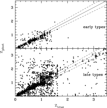
Fig. 2 shows the recovered photometric redshifts versus the true redshifts in the input catalogue for 23 256 mock galaxies with mR < 25, split by the recovered best-fitting SED template type (early or late). The figure shows a generally satisfying agreement between the input redshift and the recovered photometric redshift, especially for early-type objects. The photometric redshifts for late-type galaxies are less well constrained, presumably due to the lack of characteristic structures such as the 4000 Å Balmer break in early-type galaxy spectra. There are preferred ranges for the photometric redshift, clearly visible as horizontal bands in the diagram, presumably indicative of redshifts at which characteristic breaks in the SED fall between neighbouring filters. It is worth pointing out that this is how purely Gaussian errors in the photometry propagate, i.e. assuming a Gaussian distribution for photometric redshift errors is, in general, a fallacy.
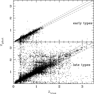
Best-fitting photometric redshifts recovered by our LF algorithm from the mock galaxy catalogue. Upper panel: galaxies best fitted with early-type templates. Bottom panel: galaxies best fitted with late-type templates.
The standard deviation of the redshift residual (zphoto−ztrue)/(1 +ztrue) for all galaxies down to m= 25 is σ= 0.40 (including catastrophic outliers); when rejecting outliers of 3σ or more, the residual standard deviation is σ= 0.059 (with 13 per cent of the objects having been rejected as outliers). The accuracy is slightly better for the early types (σ= 0.048) than for the late types (σ= 0.061). There is a slight systematic offset of Δz/(1 +z) = 0.005 (0.002 for early types and 0.005 for late types).
3.6.3 Luminosity function recovery
We will now demonstrate that our algorithm is able to recover the LF from the mock galaxy catalogue by carrying out three different analyses of the mock catalogue. As the mock catalogue is populated using a semi-analytic galaxy formation model, and not a model Schechter function, we need to recover parameters for the ‘true’ LF from the catalogue first. We do this by constraining mock galaxies to their true redshift and the best-fitting SED and absolute magnitude at that redshift. In the second analysis, we will use the best-fitting photometric redshift, SED and absolute magnitude, equivalent to the conventional approach of substituting photometric for spectroscopic redshifts. The third analysis will consist of applying the full PML formalism to the mock catalogue.

 and Mtrue are the values to which a given galaxy is constrained; this approach is similar to the original one by Marshall et al. (1983). In the calculation of the second term in equation (8), we calculate λ(f) as previously (an integral over all of observable space), but apply a hard cut-off at the survey magnitude limit without allowing for photometric uncertainties. This procedure is then equivalent to running the Marshall method on a parameter space comprising z, M and
  , rather than observed fluxes.
For each of the three analyses, we then follow the procedure that we will subsequently apply to the real data: we model the LF as a function of two SED types (early and late) in 10 redshift bins. Over the range 0.1 ≤z < 1.2 (redshift bins 2–6), we describe it in terms of equation (10), with a constant faint-end slope α and a two-parameter model for M* and its evolution with redshift for each SED type. The normalization parameters Φ* are independent in all bins; Φ* are included in the optimization in redshift bins 7 and 8. All other LF parameters, specifically in the lowest and highest redshift bins, are held constant during the optimization, but periodically readjusted to match extrapolations from the constrained bins.
An added complication is that the early-type LF in the input mock catalogue is not a single Schechter function, but exhibits a possible bimodality and a sharp cut-off at Mr=−16, neither of which is represented by the LF models that we are fitting. However, this complication will affect all three analysis methods.
Fig. 3 shows the 68 per cent and 95 per cent error contours in the α–M*0 plane for all three analyses: the calculation based on the true redshifts in dotted lines, the calculation using best-fitting photo-zs in solid thin lines and the PML solution in thick lines. Both for early- and late-type populations, the conventional approach, using best-fitting photo-zs, fails to recover the correct LF parameters in the M*–α plane. Although the fits would appear consistent if projected only on to the M* axis, a comparison involving only M* must be carried out at the same α, in which case the discrepancy between the photo-z-based solution and the true LF is even more apparent.
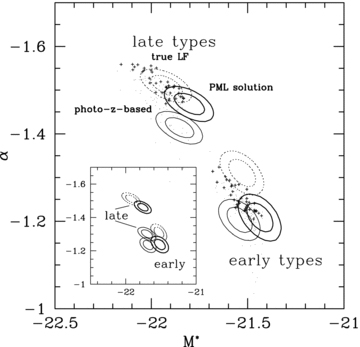
Uncertainty contours at the 68 per cent and 95 per cent levels for the LF parameters recovered from the mock catalogue using true redshifts (dotted contours), best-fitting photo-zs (thin solid contours) and the PML algorithm (thick solid contours). The main panel shows the results from UBVRIzJK filter photometry and the inset shows only BVRIz. Dots and crosses demonstrate how fluctuations in the high- and low-redshift LF parameters not included in the optimization may propagate into the recovered LF parameters, as described in the text (crosses symbolize a likelihood equal to or better than the default scenario). The photo-z-based LFs are inconsistent with the true LF, while the PML solution overlaps with the true LF in at least the 2σ level. The distribution of crosses shows that different LF priors in the lowest and highest redshift bins might bring the LF solutions in almost perfect agreement. The performance differences between photo-z-based calculations and the PML are particularly striking for the smaller filter set.
The late-type LF parameters recovered by the PML, on the other hand, are consistent with the solution obtained from the true redshifts. For the early-type population, there is a discrepancy in α, so that the 2σ contours barely overlap; however, for an α≈−1.25, which is consistent with both the PML analysis and the true redshift calculation, the recovered M* are also perfectly consistent, unlike the conventional, photo-z-based solution, which is significantly brighter.
The PML solution can be brought into even better agreement for different choices of values for the constant background parameters at very low and high redshifts. We have carried out the procedure described in Section 3.4 to determine how uncertainties in the LF priors in the very high- and low-redshift bins propagate into the LF fit. For each trial calculation, we apply Gaussian perturbations of the order of 1 mag to the M* background parameters (i.e. those not included in the optimization), and of the order of unity to the quantity  (i.e. M* typically scatter randomly within 1 mag and Φ* within a factor of 10 from the default values, which are very generous assumptions). We then calculate the best-fitting solution for the constrained parameters.
The best-fitting results of these Monte Carlo trials are shown in Fig. 3 with dots (for all fits) and crosses (for those fits that yield an equivalent or better likelihood after optimization than our default scenario). Each symbol represents one Monte Carlo trial with a different LF prior in the low- and high-redshift bins, after the maximum likelihood optimization of the free parameters has been carried out.
A large fraction of the Monte Carlo trials yield a better total likelihood than our default fit. Since we do not apply any prior to judge which of the various background LF parameters that are probed by the Monte Carlo algorithm are realistic and because, for reasons discussed in greater detail in Section 4.3, we do not consider our data set to be ideally suited for constraining the high-redshift LF, we do not actually prefer any of the Monte Carlo trials with better likelihood to our default fit; however, regardless of whether the background LFs assumed for the Monte Carlo trial is realistic or not, runs that yield a best-fitting likelihood that is significantly worse than our default scenario can be ruled out; therefore, only the crosses in Fig. 3 should be considered.
We find that, of the Monte Carlo trials that result in an equivalent or better likelihood than the default fit, almost all yield LF parameters that are in even better agreement with the true LF; in fact, for some background priors, we recover LF parameters that are in almost perfect agreement with the input LF (we have not introduced criteria, however, to decide whether the background LF priors corresponding to these trials are physically plausible or not, which is why we do not elect any of these as the real best fit). Conversely, of those LF parameters that are in worse agreement with the true LF than the default fit, almost all are marked by having a substantially worse likelihood and are thus ruled out. This means that the PML still has some constraining power in redshift regions that we have chosen not to include in our optimization in our conservative approach.
However, the Monte Carlo approach does not open up additional degrees of freedom to the photo-z-based algorithm, because (at least if the photo-zs are derived from frequentist best-fitting estimates) each galaxy is uniquely associated with a given redshift bin, independently of the LF assumed for it. Therefore, the photo-z-based LF remains clearly inconsistent with the true LF.
The advantage of the PML method over the use of photometric redshifts is even more obvious if we reduce the number of filter bands. Using only the BVRIz filters, we recover the results shown in the inset in Fig. 3. Here, the photo-z-based results are drastically different from the ‘true’ LFs; the late-type LF is found to be α≈−1.3, compared to the actual α=−1.52, and the recovered early-type LF is also significantly brighter and shallower than the input LF. In contrast, the uncertainty contours of the PML solution again overlap with those of the ‘true’ LF.
4 RESULTS AND DISCUSSION
4.1 Magnitude limits
How deep does MUSYC probe the galaxy LF in our individual redshift bins? To answer this question, we plot in Fig. 4 the derivative of the second term of the likelihood function in equation (8) with respect to the value Φ(M) of the LF at a given absolute magnitude; this is, in essence, the volume over which a galaxy with a given SED and absolute magnitude in a given redshift bin would be visible. It has here been normalized to unity for the brightest galaxies. The figure shows the completeness for the earliest- and the latest-type SED in redshift bins 2 (0.1 ≤z < 0.25), 3 (0.25 ≤z < 0.4), 4 (0.4 ≤z < 0.6), 6 (0.8 ≤z < 1.2) and 8 (1.5 ≤z < 2.5).
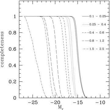
Effective r-band magnitude limits for five of our 10 redshift bins. Different line styles indicate different redshift bins. For each redshift bin, we draw two completeness curves, corresponding to very late and very early types. Assignment of line styles to redshift ranges is given in the plot.
For higher redshifts, the early- and late-type completeness curves differ significantly, indicating that late-type galaxies are more easily detectable than early-type ones. The curves do not cut off abruptly at a given absolute magnitude due to the fact that each redshift bin has a finite extent in redshift; galaxies near the low-redshift boundary of a bin are visible to fainter absolute magnitudes than those at the high-redshift boundary. In the lowest redshift bin under analysis here, our sensitivity extends to MR≈−14.
4.2 Photometric redshift and luminosity recovery
We have already demonstrated that the PML is capable of recovering the redshift of galaxies in the mock catalogue. In the application to real data, additional systematic errors that are not modelled by the mock catalogue may come into play, such as systematic biases in the photometry that our zero-point corrections may not have sufficiently compensated for. The best-fitting photometric redshifts recovered by our algorithm are a convenient way of testing for the presence of such serious systematic errors. For this comparison, we have drawn spectroscopic redshifts in the E-CDFS field from various public and proprietary sources, including the NASA Extragalactic Database (NED), publications by Ravikumar et al. (2007) and Vanzella et al (2008), as well as redshifts determined within the MUSYC project, yielding a total of 2602 redshifts.
Fig. 5 shows the performance of the recovered best-fitting photometric redshifts versus spectroscopic redshifts. The plot resembles our previous comparison using the mock catalogues in Fig. 2: the performance is generally good; late-type objects suffer from more catastrophic failures. The standard deviation of the redshift residual (zphoto−ztrue)/(1 +ztrue) is σ= 0.27 (including catastrophic outliers); when rejecting outliers of 3σ or more, the residual standard deviation is σ= 0.062 (with 17 per cent of the objects having been rejected as outliers). The accuracy is similar for early types (σ= 0.061) and for late types (σ= 0.063). For comparison, prior to applying our photometric corrections to the zero-points and uncertainties, these numbers are σ= 0.32 and σ= 0.082, respectively (σ= 0.077 for early types and σ= 0.083 for late types).
Best-fitting photometric redshifts compared to known spectroscopic redshifts in the MUSYC catalogue. Upper panel: galaxies best fitted with early-type templates. Bottom panel: galaxies best fitted with late-type templates.
Comparison between Figs 2 and 5 shows that many of the structures (particularly the horizontal patterns showing preferred values for photometric redshifts) found in the real mock data are visible in the observed data as well. This provides important verification that the pattern of catastrophic failures in the photometric redshift recovery can be reproduced on the basis of just the Gaussian errors in the input photometry and that, therefore, such colour degeneracies, which normally present a grave problem for photo-z-based LF determines can be accounted for naturally by the PML.
However, there is an indication of photo-zs of early-type galaxies being systematically underestimated at z > 1; this feature is only partially reproduced by the mock data and thus not fully corrected for by the PML either. Therefore, we restrict our analysis to the redshift range 0.1 ≤z < 1.2, the last redshift bin covering the fairly wide range 0.8 ≤z < 1.2.
The fact that our photometric data and SED template set allow us recover photometric redshifts with acceptable accuracy is encouraging, even though our algorithm does not use individual photometric redshifts per se. For the purpose of calculating LFs, the ability to recover the absolute magnitude of a galaxy and account for k-corrections and other cosmological effects is at least as important. Although, unlike the redshift, the absolute magnitude cannot be verified by alternate observations, the COMBO-17 survey (Wolf et al. 2004) offers a high-quality comparison catalogue that covers the same field and contains estimates of absolute magnitudes in the r band. Cross-matching the COMBO-17 catalogue and the MUSYC catalogue yields 26 234 galaxies. After adding an offset of 0.055 mag to the COMBO-17 R-band magnitudes to convert from the Vega to the AB system (Frei & Gunn 1994), the apparent magnitudes in both catalogues agree well apart from a systematic offset of mMUSYC−mCOMBO-17≈+0.045 (in the R band; total magnitudes for COMBO-17 and either corrected aperture or auto magnitudes for MUSYC, as described in Section 2).
To evaluate our ability to recover absolute magnitudes from the MUSYC photometric data, we now constrain the MUSYC galaxies to be at the photometric redshift listed in the COMBO-17 catalogue and carry out an SED fit at that redshift to calculate the r-band rest-frame absolute magnitude. For a given redshift and SED type, the PML calculates the rest-frame luminosity of a galaxy directly from the normalization factor that yields the best fit of the SED to the observed fluxes. We compare these absolute magnitudes to the r band estimates provided by Wolf et al. (2008) by calculating the quantity (MMUSYC−MCOMBO- 17) − (mMUSYC−mCOMBO- 17), which accounts for the measured differences in observer-frame R-band apparent magnitudes to isolate only the differences in the recovered absolute magnitude. Offsets between the AB and Vega systems are negligible in the rest-frame r band (Frei & Gunn 1994). We restrict this comparison to galaxies with R < 22, because fainter galaxies (R > 22.5) in the COMBO-17 catalogue exhibit a strong quantization in the best-fitting photometric redshifts that casts doubts on their reliability. We then find a mean of ∼−0.06 with a dispersion of 0.22 over the redshift range 0.1 ≤z < 1.0, i.e. MUSYC galaxies are inferred to be slightly more luminous at the same redshift and for the same rest-frame R-band magnitude. This value is only very weakly dependent on redshift (with a slope of −0.05 and a zero point of −0.04 at z= 0). A small contribution to this discrepancy may come from differences in the cosmological model in the calculation of absolute magnitudes (Ωλ= 0.73 and Ωm= 0.27 in our study, Ωλ= 0.7 and Ωm= 0.3 for COMBO-17); this difference is ∼0.04 mag at z= 1 in the sense of MUSYC galaxies being inferred to be brighter. Therefore, if residual systematic discrepancies exist in our calculation of absolute rest-frame magnitudes in comparison to COMBO-17, they are at the level of <0.1 mag for the redshift range that we are analysing. Possible reasons for this residual discrepancy include the fact that our rest-frame luminosities are constrained by all available filter bands, so that the subtraction of the (mMUSYC−mCOMBO- 17) term in the R band will not account for all discrepancies in the input photometry, as well as the different template set.
4.3 The cosmic luminosity function
We now apply the PML to the MUSYC data to calculate the field galaxy LF. For this purpose, we use the parametrization given by equation (10), i.e. for each of the two SED classes, we assume a characteristic bright-end magnitude M*0 at a fiducial redshift z= 0.95 (experimentally found to be the redshift for which M* is constrained best in this sample), a faint-end slope α and an evolutionary parameter δ to describe the variation of M* with redshift according to M*=M*0−δ× lg[(1 +z)/(1 +z0)]. The normalization parameters Φ* are independent for each redshift bin and SED class. For the present work, we have chosen to calculate the LFs in the rest-frame r band. This band is less sensitive to effects of current star formation than, for example, the B band, but at the same time it is well constrained by the available photometry over the redshift range of particular interest to us.
The purpose of this calculation is to recover an approximate representation of the LF, albeit with a low number of free parameters, which will serve as the starting point for a subsequent refinement with a more detailed ansatz. Furthermore, we will use this calculation to constrain the faint-end slopes α for the early and late SED types from this calculation and adopt them for the rest of the analysis. While it would be possible to optimize with respect to the faint-end slopes α in individual redshift bins, the flux limit prevents us from obtaining useful constraints on α in any but the lowest redshift bins, up to z≈ 0.4–0.5. A follow-up study of a larger sample will explore this issue.
Parameters that we include in the optimization are M*0, α and δ for both SED types, describing the shape of the LF over the range 0.1 ≤z < 1.2. Furthermore, we constrain Φ* over the range 0.1 ≤z < 2.5. All other LF parameters (i.e. α, M* in redshift bins 1 and 7 to 10 and Φ* in bins 1, 9 and 10) are held constant. The decision to treat the high-redshift LF parameters as constant background parameters is based on a number of criteria as follows.
The rest-frame r band is not constrained directly by the available filter complement at high redshift.
Only the tip of the LF is sampled, which may introduce strong systematic errors if the most luminous galaxies do not obey the same Schechter function implied for the bulk of the galaxy population.
The applicability of z= 0 empirical templates to high-redshift galaxy populations is doubtful.
Photometric redshifts, using this catalogue and our template set, have proven much less reliable at z > 1.0, as is also shown by Figs 2 and 5.
At low redshift, on the other hand, constraints on the LF are weak due to the small number of galaxies and the large uncertainties affecting the absolute magnitudes of individual galaxies.
The initial values that we choose for these background parameters are motivated by the results of Giallongo et al. (2005). Their work uses two different criteria to separate early- and late-type galaxies – colours and specific star formation rate – and examines two ways of defining the threshold values – empirically, from the observed bimodality or from a theoretical evolutionary track. This yields four different estimates for the LF and its evolution for a given galaxy type. To obtain an estimate in a given redshift bin, we evaluate their fit at the central redshift of the bin and average the four extrapolated values for M* and Φ*. To convert their B-band LFs into our r-band rest-frame absolute magnitudes, we adjust M* by B−r= 1.35 for early types and B−r= 0.9 for late types. These values correspond to typical B−r colors for early and late populations from Wolf et al. (2003) at low redshift. We caution that the distinction made by Giallongo et al. between early and late types is different from ours; in particular, while we use redshift-zero SED templates to fit early- and late-type LFs, their threshold values for parameters such as colour and specific star formation rate vary with redshift. We therefore expect that ‘early’ types would be more prevalent at high redshift according to their definition than to ours.
We repeat the best-fitting search several times; after each iteration, we adjust the background parameters by averaging their previous values with linear extrapolations of the best-fitting M* and Φ* values over lg(1 +z). Above the last redshift bin directly constrained by our fit (above z= 2.5), we cap the extrapolated values for these parameters at those found in the closest redshift bin where they are constrained directly, so as to avoid implying unrealistically bright or abundant galaxy populations in the high-redshift Universe.
We solve for the maximum likelihood solution in the remaining 16-parameter space [two SED types × (three shape parameters + seven normalization parameters)] using an iterative algorithm that, starting from the previous solution, first searches for the maximum likelihood point along each parameter axis, thus deriving a shift Δpi in each parameter pi. Subsequently, it applies a shift xΔp to all parameters simultaneously and calculates the likelihood as a function of the scaling factor x in the same manner. If the resulting adjustment in any given parameter is much smaller than the spacing between the trial points that are initially evaluated along the parameter axis, this spacing is slightly reduced. The algorithm stops when the trial point spacings along all parameter axes are much smaller than the typical statistical uncertainties.
The best-fitting values for the 16 parameters included in the optimization are given in Table 3, along with the values adopted for the constant ‘background’ parameters. The projection of the α–M*0 plane is shown in Fig. 6, along with the 68 per cent and 95 per cent error contours. Here, bold error contours indicate the results of the PML analysis, while thin lines represent the classical calculation using fixed photo-zs; the uncertainty regions are clearly disjunct.
LF results at 0.1 ≤z < 1.2.
| Bin | z | α | M* | δ | lg Φ* |
| Early types | |||||
| – | – | −0.62+0.04−0.06 | −21.885+0.075−0.075 | 0.107+0.780−0.720 | – |
| 1 | 0.02 – 0.10 | −0.639 | −21.918 | – | −2.502 |
| 2 | 0.10 – 0.25 | –. | – | – | −2.321+0.043−0.037 |
| 3 | 0.25 – 0.40 | – | – | – | −2.726+0.044−0.039 |
| 4 | 0.40 – 0.60 | – | – | – | −2.632+0.034−0.026 |
| 5 | 0.60 – 0.80 | – | – | – | −2.482+0.025−0.020 |
| 6 | 0.80 – 1.20 | – | – | – | −2.756+0.028−0.027 |
| 7 | 1.20 – 1.50 | −0.639 | −21.867 | – | −2.709+0.053−0.056 |
| 8 | 1.50 – 2.50 | −0.639 | −21.849 | – | −2.685+0.077−0.079 |
| 9 | 2.50 – 3.50 | −0.639 | −21.828 | – | −2.850 |
| 10 | 3.50 – 6.00 | −0.639 | −21.802 | – | −2.953 |
| Late types | |||||
| – | – | −1.62+0.02−0.02 | −22.345+0.075−0.100 | 2.484+1.260−1.500 | – |
| 1 | 0.02 – 0.10 | −1.664 | −21.683 | – | −3.158 |
| 2 | 0.10 – 0.25 | – | – | – | −2.924+0.025−0.057 |
| 3 | 0.25 – 0.40 | – | – | – | −3.144+0.029−0.064 |
| 4 | 0.40 – 0.60 | – | – | – | −3.078+0.017−0.061 |
| 5 | 0.60 – 0.80 | – | – | – | −3.029+0.013−0.064 |
| 6 | 0.80 – 1.20 | – | – | – | −3.123+0.018−0.067 |
| 7 | 1.20 – 1.50 | -1.664 | −22.749 | – | −3.688+0.066−0.085 |
| 8 | 1.50 – 2.50 | −1.664 | −22.967 | – | −2.769+0.008−0.006 |
| 9 | 2.50 – 3.50 | −1.664 | −22.967 | – | −3.252 |
| 10 | 3.50 – 6.00 | −1.664 | −22.967 | – | −3.280 |
Results from the fit of SED-specific Schechter functions to the redshift range 0.1 ≤z < 1.2. In the first row of each section of the table, we give the shape parameters describing the best-fitting LF in this range. Normalization parameters Φ* are listed separately for each redshift bin. Values without uncertainties are constant background values and not optimized. The parameter M* is evaluated at z= 0.95.
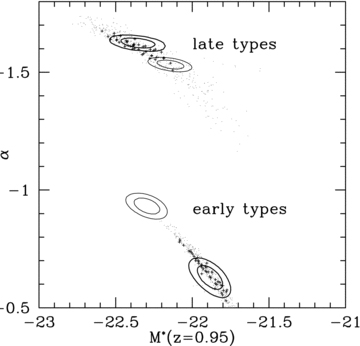
Uncertainty contours for the best-fitting LF parameters at 68 per cent and 95 per cent confidence levels in the α–M* parameter space. Bold contour lines show the PML solution, while thin contour lines indicate a solution based on a conventional algorithm using best-fit photo-zs. The results reflect a dichotomy between the early-type LF with a shallow faint-end slope and the late-type LF with an extremely steep slope of α≈−1.6. Dots and crosses again demonstrate how fluctuations in the high- and low-redshift LF parameters propagate into the recovered LF parameters. Only trial runs symbolized with crosses yield an acceptable likelihood.
The qualitative behaviour of the fits is consistent with many previous literature results (i.e. Bromley et al. 1998; Wolf et al. 2003) regarding the late- and early-type LFs, whose most important characteristics are a rather shallow slope for early-type galaxies and a significantly steeper slope for late-type galaxies. However, the steepness of the slope of our late-type LF is remarkable indeed; we find −1.62+0.02−0.02, compared to −0.62+0.04−0.06 for the early types. Literature values for the total LF tend to prefer values of α=−1.2 to −1.3. However, it is also known that the late-type LF is steeper than this average, and Blanton et al. (2005) find α=−1.3 in the SDSS, but speculate (based on the fact that the SDSS is likely to miss many low-surface brightness objects) that it may be as steep as −1.5 or even steeper. Such steep slopes at the faint end can be easily reconciled with older values of α≈−1.2 by noting that the bright end of the LF is dominated by early-type galaxies and that the late-type LF with its steep slope will begin to dominate the total LF at several magnitudes fainter than M*, i.e. only surveys combining very deep samples with sufficient statistics to constrain the extreme faint end will be able to identify this as an upturn. It is conceivable that this dichotomy may also be identified as a ‘dip’ in the overall LF, especially in denser environments, where the steep late-type LF is likely to have been depleted by environmental processes and its normalization Φ* lowered. Indeed, claims of such a ‘dip’ feature in the overall LF have been raised in the past based on surveys of galaxy groups (Flint et al. 2003; Mendes de Oliveira et al. 2006; Miles et al. 2006) and the Coma cluster (Biviano et al. 1996).
The early- and late-type populations show a very different evolutionary behaviour with redshift. For the early-type sample, we find δ≈ 0, i.e. no evidence for luminosity evolution up to z= 1.2. In contrast, the late-type sample is fitted by an evolving LF with δ≈ 2.5, i.e. M* brightens by about 0.75 mag from z= 0 to z= 1. However, the uncertainties on the δ parameters are very large, and even the late-type sample is formally consistent with very weak luminosity evolution.
Our two-parameter fit to M*(z) can be extrapolated to z= 0 to recover the local LF parameters; however, as M* is primarily constrained by galaxies at z≈ 0.95, uncertainties in δ propagate strongly into the extrapolated value. Formally, we find M*(z= 0) =−21.854+0.200−0.200 for the early-type and M*(z= 0) =−21.632+0.340−0.400 for the late-type population. However, better constraints on the LF at z= 0 can be obtained by fitting the LF parameters directly in individual low-redshift bins, and we refer the reader to Section 4.4, where we will discuss this question in greater detail.
As we have discussed in Section 3.4, we presume LF parameters at very low and very high redshifts to be constant instead of constraining them directly from the data, as they are very susceptible to systematic errors. However, as LF parameters in different redshift bins are usually covariate, the exact LF solution recovered here depends on our assumptions for the values of these background parameters. We have applied the Monte Carlo approach described in Section 3.4 to gauge the sensitivity of the best-fitting parameters to these background values. For each trial calculation, we apply Gaussian perturbations of the order of 1 mag to the M* background parameters and of the order of unity to the quantity  in these background bins (i.e. M* typically scatter randomly within 1 mag and Φ* within a factor of 10 from the default values). We then calculate the best-fitting solution for the constrained parameters. The results are shown in Fig. 6 in the M*0–α plane. Dots represent Monte Carlo runs for which the final, best-fitting likelihood is substantially worse than for our default values; this means that the corresponding configuration of background parameters is ruled out by the data and the run can be discarded. Crosses represent those runs for which we achieve a similar or better maximum likelihood than for our default background choices; these represent background configurations that cannot be ruled out by the data, although we do not judge whether the configuration of background LFs assumed in each Monte Carlo trial is realistic and therefore do not prefer any of these solutions to our default scenario. According to Fig. 6, variations in the background parameters may then introduce a scatter that exceeds the 2σ uncertainty contours. However, the qualitative picture remains unchanged; in particular, none of the acceptable Monte Carlo trials yields α > −1.5 for the late-type population. Furthermore, only a very few outliers in the Monte Carlo analysis yield LF parameters consistent with the photo-z-based calculation for the late-type population, and none of them is consistent with the photo-z-based early-type LF. We furthermore point out that the amount by which the background parameters are allowed to scatter from the default assumption is very generous. We interpret this as indicating that, to change the faint-end slope α of the late-type population to values shallower than −1.5, Φ* at high redshift would have to be permitted to deviate by more than a factor of 10 upwards from the values found at lower redshift or M* by more than a magnitude towards the bright end, i.e. the high-redshift galaxy population would have to be much brighter and more abundant than at z < 1.2, which is a scenario that we consider unrealistic.
In order to test the effect of excluding detections with questionable star/galaxy classifications, we have carried out an alternate fit including only objects with S/G≤ 0.8 (as opposed to our default of 0.97). The resulting best-fitting values differ slightly from those obtained above; most notably, M*0 for the early types is fainter at M*0=−21.62 and the faint-end slope is slightly shallower at α=−0.43. However, there is virtually no change in the late-type LF, where the best-fitting values are M*0=−21.66 and α=−1.61. As α and M*0 are correlated, it is not immediately clear whether the shift in the early-type best-fitting parameters is due to a change at the bright or the faint end; however, as there is no obvious tendency for objects with S/G > 0.8 to be associated with unusually high luminosities, we suspect that the change is due to the removal of compact sources with photometric properties characteristic of low-redshift early-type objects. We return to this question once more in Section 4.7, where we analyse the shape of the LF in a binned representation.
Just as doubts regarding the appropriateness of our empirical SED templates prevent us from constraining the LF in the high-redshift Universe, we may also wonder whether a mismatch between our late-type templates and the photometric properties of dwarf galaxies may have steepened the observed faint-end slope artificially. Dwarf galaxies, typically being of low metallicity, may have significantly different spectral properties than the brighter objects that the CWW templates were originally drawn from. However, we would expect template insufficiency to lower the recovered LF value associated with the galaxy populations that are not represented well by the template, while the LF of other populations with similar photometric properties would be boosted instead. Therefore, a greater concern regarding the steep faint end lies with the question whether the high-redshift LF is represented well by our templates. The Monte Carlo procedure described above, however, demonstrates that the steep faint-end slope is not very sensitive to the LF values assumed for the high-redshift population and cannot be pushed to values shallower than α≈−1.5 even for the rather large background fluctuations assumed there.
4.4 The luminosity function in individual redshift bins
Our best-fitting solution described in Section 4.3 has been based on a relatively low number of free parameters. One of the disadvantages incurred by this is that the constraints on M* are weak and the extrapolation to redshift zero via the two parameters M*0 and δ is potentially affected by large errors. Furthermore, our assumptions (such as the simple two-parametric model for M* as a function of redshift) cannot be verified explicitly within the confines of this simple approach.
To explicitly test these assumptions and obtain more accurate constraints on the LF at low redshift, we now refine our solution by maximizing the likelihood with respect to the parameters M* and Φ* in individual redshift bins. We iterate both parameters for each SED type and for each redshift bin. Other than that, the same parameters are included in this optimization as in the previous section: Φ* in redshift bins 7 and 8 and the faint-end slope α in bins 2–6 (assumed independent of redshift).
The results of this analysis – in an M*–Φ* projection – are shown in Fig. 7. Bold contours represent early types and thin contours late types. Error contours are calculated for two degrees of freedom and 68 per cent confidence. Table 4 gives the best-fitting values in individual redshift bins.
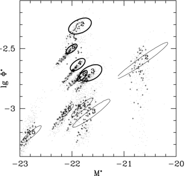
Uncertainty contours at the 68 per cent confidence level for fits to the early-type (bold contours) and late-type (light contours) LF in individual redshift bins over the range 0.1 ≤z < 1.2. For the early-type LF, we see no evidence for an evolution of M*, while Φ* exhibits considerable scatter, which may be associated with known density inhomogeneities in the E-CDFS. The late-type LFs exhibit a strong covariance between M* and Φ* and populate a sequence ranging from faint M*/high Φ* at low to bright M*/low Φ* at high redshift, attesting to evolution in at least one parameter. Dots and crosses illustrate how variations in the constant high- and low-redshift LF parameters may propagate into the recovered LFs.
LF results at 0.1 ≤z < 1.2.
| Bin | z | α | M* |  | |
| Early types | |||||
| 1 | 0.02 – 0.10 | −0.639 | −21.92 | −2.502 | |
| 2 | 0.10 – 0.25 | −0.640 | −21.84+0.20−0.20 | −2.311+0.063−0.063 | |
| 3 | 0.25 – 0.40 | −0.640 | −21.64+0.20−0.20 | −2.702+0.063−0.063 | |
| 4 | 0.40 – 0.60 | −0.640 | −21.89+0.13−0.13 | −2.633+0.038−0.050 | |
| 5 | 0.60 – 0.80 | −0.640 | −22.01+0.10−0.10 | −2.502+0.038−0.038 | |
| 6 | 0.80 – 1.20 | −0.640 | −21.80+0.07−0.07 | −2.727+0.038−0.037 | |
| 7 | 1.20 – 1.50 | −0.639 | −21.87 | −2.721+0.051−0.055 | |
| 8 | 1.50 – 2.50 | −0.639 | −21.85 | −2.694+0.071−0.079 | |
| 9 | 2.50 – 3.50 | −0.639 | −21.83 | −2.850 | |
| 10 | 3.50 – 6.00 | −0.639 | −21.80 | −2.953 | |
| Late types | |||||
| 1 | 0.02 – 0.10 | −1.664 | −21.68 | −3.158 | |
| 2 | 0.10 – 0.25 | −1.637 | −20.60+0.43−0.50 | −2.588+0.138−0.150 | |
| 3 | 0.25 – 0.40 | −1.637 | −21.62+0.32−0.35 | −3.037+0.100−0.112 | |
| 4 | 0.40 – 0.60 | −1.637 | −21.80+0.18−0.20 | −2.987+0.063−0.075 | |
| 5 | 0.60 – 0.80 | −1.637 | −22.77+0.17−0.18 | −3.212+0.063−0.063 | |
| 6 | 0.80 – 1.20 | −1.637 | −22.08+0.10−0.10 | −3.017+0.050−0.050 | |
| 7 | 1.20 – 1.50 | −1.664 | −22.75 | −3.633+0.070−0.081 | |
| 8 | 1.50 – 2.50 | −1.664 | −22.97 | −2.700+0.006−0.007 | |
| 9 | 2.50 – 3.50 | −1.664 | −22.97 | −3.252 | |
| 10 | 3.50 – 6.00 | −1.664 | −22.97 | −3.280 | |
| Bin | z | α | M* | | |
| Early types | |||||
| 1 | 0.02 – 0.10 | −0.639 | −21.92 | −2.502 | |
| 2 | 0.10 – 0.25 | −0.640 | −21.84+0.20−0.20 | −2.311+0.063−0.063 | |
| 3 | 0.25 – 0.40 | −0.640 | −21.64+0.20−0.20 | −2.702+0.063−0.063 | |
| 4 | 0.40 – 0.60 | −0.640 | −21.89+0.13−0.13 | −2.633+0.038−0.050 | |
| 5 | 0.60 – 0.80 | −0.640 | −22.01+0.10−0.10 | −2.502+0.038−0.038 | |
| 6 | 0.80 – 1.20 | −0.640 | −21.80+0.07−0.07 | −2.727+0.038−0.037 | |
| 7 | 1.20 – 1.50 | −0.639 | −21.87 | −2.721+0.051−0.055 | |
| 8 | 1.50 – 2.50 | −0.639 | −21.85 | −2.694+0.071−0.079 | |
| 9 | 2.50 – 3.50 | −0.639 | −21.83 | −2.850 | |
| 10 | 3.50 – 6.00 | −0.639 | −21.80 | −2.953 | |
| Late types | |||||
| 1 | 0.02 – 0.10 | −1.664 | −21.68 | −3.158 | |
| 2 | 0.10 – 0.25 | −1.637 | −20.60+0.43−0.50 | −2.588+0.138−0.150 | |
| 3 | 0.25 – 0.40 | −1.637 | −21.62+0.32−0.35 | −3.037+0.100−0.112 | |
| 4 | 0.40 – 0.60 | −1.637 | −21.80+0.18−0.20 | −2.987+0.063−0.075 | |
| 5 | 0.60 – 0.80 | −1.637 | −22.77+0.17−0.18 | −3.212+0.063−0.063 | |
| 6 | 0.80 – 1.20 | −1.637 | −22.08+0.10−0.10 | −3.017+0.050−0.050 | |
| 7 | 1.20 – 1.50 | −1.664 | −22.75 | −3.633+0.070−0.081 | |
| 8 | 1.50 – 2.50 | −1.664 | −22.97 | −2.700+0.006−0.007 | |
| 9 | 2.50 – 3.50 | −1.664 | −22.97 | −3.252 | |
| 10 | 3.50 – 6.00 | −1.664 | −22.97 | −3.280 | |
Best-fitting LF parameters in individual redshift bins. Fits are carried out in bins 2–8. Best-fitting values for Φ* in redshift bins 7 and 8 are shown for completeness, but lie beyond the reliable redshift region.
LF results at 0.1 ≤z < 1.2.
| Bin | z | α | M* | | |
| Early types | |||||
| 1 | 0.02 – 0.10 | −0.639 | −21.92 | −2.502 | |
| 2 | 0.10 – 0.25 | −0.640 | −21.84+0.20−0.20 | −2.311+0.063−0.063 | |
| 3 | 0.25 – 0.40 | −0.640 | −21.64+0.20−0.20 | −2.702+0.063−0.063 | |
| 4 | 0.40 – 0.60 | −0.640 | −21.89+0.13−0.13 | −2.633+0.038−0.050 | |
| 5 | 0.60 – 0.80 | −0.640 | −22.01+0.10−0.10 | −2.502+0.038−0.038 | |
| 6 | 0.80 – 1.20 | −0.640 | −21.80+0.07−0.07 | −2.727+0.038−0.037 | |
| 7 | 1.20 – 1.50 | −0.639 | −21.87 | −2.721+0.051−0.055 | |
| 8 | 1.50 – 2.50 | −0.639 | −21.85 | −2.694+0.071−0.079 | |
| 9 | 2.50 – 3.50 | −0.639 | −21.83 | −2.850 | |
| 10 | 3.50 – 6.00 | −0.639 | −21.80 | −2.953 | |
| Late types | |||||
| 1 | 0.02 – 0.10 | −1.664 | −21.68 | −3.158 | |
| 2 | 0.10 – 0.25 | −1.637 | −20.60+0.43−0.50 | −2.588+0.138−0.150 | |
| 3 | 0.25 – 0.40 | −1.637 | −21.62+0.32−0.35 | −3.037+0.100−0.112 | |
| 4 | 0.40 – 0.60 | −1.637 | −21.80+0.18−0.20 | −2.987+0.063−0.075 | |
| 5 | 0.60 – 0.80 | −1.637 | −22.77+0.17−0.18 | −3.212+0.063−0.063 | |
| 6 | 0.80 – 1.20 | −1.637 | −22.08+0.10−0.10 | −3.017+0.050−0.050 | |
| 7 | 1.20 – 1.50 | −1.664 | −22.75 | −3.633+0.070−0.081 | |
| 8 | 1.50 – 2.50 | −1.664 | −22.97 | −2.700+0.006−0.007 | |
| 9 | 2.50 – 3.50 | −1.664 | −22.97 | −3.252 | |
| 10 | 3.50 – 6.00 | −1.664 | −22.97 | −3.280 | |
Best-fitting LF parameters in individual redshift bins. Fits are carried out in bins 2–8. Best-fitting values for Φ* in redshift bins 7 and 8 are shown for completeness, but lie beyond the reliable redshift region.
The early-type galaxies exhibit relatively little scatter in M*– all error contours lie in the range −22.2 < M*r < −21.5. Given the relatively large uncertainties, there is no obvious trend of M* with redshift, confirming the conclusion that δ≈ 0. The scatter in Φ* is larger than the uncertainties; in the seven redshift bins included in our analysis, Φ* scatters within a factor of ∼3. The scatter may be affected by large-scale structure. Phleps et al. (2007) report an underdensity at 0.25 < z < 0.4, which coincides with our very low data point in redshift bin 3. On the other hand, Adami et al. (2005), based on spectroscopic data, note several structures, including massive galaxy groups, at z≈ 0.7, which falls into our redshift bin 5, which is significantly elevated in comparison to the neighbouring bins. Our LF results are therefore qualitatively consistent with large-scale structure features in the E-CDFS known from spectroscopic studies. The scatter introduced by these features is too large to permit any reliable conclusion as to whether Φ* exhibits a trend with redshift.
The uncertainty contours for the late-type LFs are affected by the strong covariance between M* and Φ* in the case of a steep faint end. The best-fitting values form an approximate sequence, with the faintest, but highest normalization fits being found at low redshift, while the high-redshift LFs are brighter by more than 2 mag in M*, but also exhibit a lower Φ* (by a factor of 2–3); this is also consistent with our earlier finding of a positive evolution parameter δ. Comparison of the corresponding Schechter profiles shows that the variation of the late-type LF between redshift bins occurs primarily at the bright end, whereas the normalization of the LFs in this redshift range is almost constant with redshift at magnitudes Mr > −20. However, redshift bin 3 deviates significantly towards lower normalizations from the sequence along which the uncertainty contours for the other bins are aligned, which is again consistent with the claim of an underdensity in the E-CDFS in this redshift range.
We have again determined the impact of varying the high- and low-redshift LF parameters held constant during these fits using a Monte Carlo procedure as described in Section 3.4. The range of best-fitting parameters is shown in Fig. 7 by dots for all trials and crosses for trials yielding acceptable likelihood. For the early-type LFs, shifts towards slightly brighter M*/lower Φ* are possible, but shifts in the opposite sense (fainter M*) are ruled out. For the late-type sample, the background uncertainties propagate primarily into variations in Φ*. We remind the reader that the magnitude of these variations is dependent on the magnitude of the high- and low-z background uncertainties, which are assumed to be very generous here (a factor of 10 in Φ* and 1 mag in M*), and that the Monte Carlo procedure can therefore only convey a qualitative impression of the robustness of the results and the sense in which they may deviate from the default solution.
4.5 Comparison to other surveys
Our results for the low-redshift LF appear to be in contrast to other determinations for the local field LF (Blanton et al. 2003); in particular, M* for the early-type population at low redshift appears strikingly bright, compared to a value of M*r=−21.18 ± 0.01 at z= 0.1 given by Blanton et al. (adjusted to H0= 71).
To illuminate the causes of this discrepancy, we present in Fig. 8 a comparison between the Blanton et al. LF at z= 0.1 and our results in four low-redshift bins, as given in Table 4. For the purpose of facilitating comparison, we have drawn the z= 0.1 Blanton et al. LF in all four panels, but emphasize that even the lowest redshift bin of our study shown here lies above the redshift for which this LF was calculated.
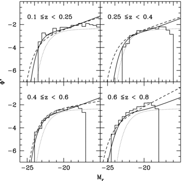
Comparison between the distribution of spectroscopically confirmed galaxies in absolute magnitude (histogram) with our LF fits to the photometric catalogue (solid line), the z= 0.1 field LF from Blanton et al. (2003) (dotted line) and LFs in similar redshift bins from Wolf et al. (2003) (dashed line). At the bright end, it confirms the shape of the PML solution. At the faint end, the observed distribution is a lower limit, because no volume correction has been applied.
The histograms show the distribution of absolute magnitudes of galaxies with known spectroscopic redshifts in the MUSYC catalogue. For bright galaxies, more than 25 per cent of the objects in the catalogue have spectroscopic redshifts; we have applied an approximate completeness correction as a function of the apparent magnitude mR and divided by the comoving volume of the redshift bin. Apart from the calculation of the rest-frame r-band absolute magnitudes, these are the only corrections applied to the data. In particular, we have abstained from applying a volume correction in order to minimize the risk of introducing systematic errors into this distribution. For this reason, the distribution of observed galaxies can only give a reasonable impression of the shape of the LF at the bright end, which is observable across the entire bin.
The observed distribution does not agree with our LFs at the faint end, which is not surprising, because no volume correction has been applied; the observed distribution is therefore likely to be a lower bound on the true LF, because the prevalence of faint galaxies, which are not visible across the entire volume of a given redshift bin, has certainly been underestimated.
None the less, Fig. 8 reveals a remarkably good agreement between our best-fitting LFs calculated with the PML and the directly observed galaxy distribution, both with regard to the shape of the bright end and the normalization. In comparison, in the lowest redshift bin, which contains the redshift of z= 0.1 for which the Blanton et al. LF holds, the observed distribution of absolute magnitudes extends to far brighter magnitudes than that the LF would permit.
The disagreement with the low-redshift LF of Blanton et al. is surprising. It cannot be due to a specific fault of our LF algorithm, because even just the absolute magnitude distribution of spectroscopically confirmed galaxies is clearly in excess of the former's prediction. The fault does not appear to lie with our calculation of absolute magnitudes either, because comparison to absolute magnitudes published in the COMBO-17 catalogue shows at most small (ΔM≈−0.06) systematics even as far as z≈ 1 and scatter in the recovered absolute magnitudes of ∼0.22, not nearly enough to push the bright end forwards by about a magnitude. At the extreme low-redshift end, our recovered absolute magnitudes are also in excellent agreement with comparison values calculated naively from the observer-frame r-band magnitudes simply by applying a distance modulus, indicating that our procedure of calculating absolute magnitudes from SED fits to all filter bands simultaneously does not introduce discrepancies from the conventional procedure of applying a k-correction to the measured photometry in a single band.
In this context, it is worth pointing out that the LFs recovered by Wolf et al. (2003) from COMBO-17 (which was obtained with the same telescope and instrument and overlaps with the E-CDFS field that we analyse here) are also significantly brighter than the Blanton et al. estimate and as bright as or even brighter than our solution. For comparison, we have overplotted the total LFs of Wolf et al. in Fig. 8 as dashed lines. In the upper left-hand and upper right-hand panels (covering the redshift ranges 0.1 ≤z < 0.25 and 0.25 ≤z < 0.4, respectively), the Wolf et al. LFs shown are those at z= 0.3 (the lowest redshift bin independently constrained by their work); in the bottom left-hand panel, it is the LF at z= 0.5; and in the bottom right-hand panel, z= 0.7, which coincides well with our choice of binning. In all bins, the Wolf et al. LF is substantially brighter than the estimate of Blanton et al. at z= 0.1 and agrees qualitatively with or is even brighter than our LF determination. The faint-end slopes in their work show considerable variance, but in the lowest redshift bin, where it may be supposed to be constrained best, it matches ours in normalization and slope.
The agreement between our work and that of Wolf et al. (2003) with regard to the bright end at low redshift being substantially brighter than estimated by Blanton et al. (2003) suggests that the depth of the photometry, and particularly the surface brightness depth, may be at least partly responsible for the brighter faint end recovered by us and Wolf et al. (2003). In particular, it is possible that the often very extended envelopes of luminous early-type galaxies, which dominate the bright tip of the LF, might be underestimated in the shallower SDSS data.
Sample variance due to a large-scale structure must also be taken into account as a possible additional contributor to the discrepancy between our LF and that of Blanton et al.; Fig. 8 attests to considerable variance from one redshift bin to the next. We do recover a significantly fainter LF in the redshift range 0.25 ≤z < 0.4 than in the 0.1 ≤z < 0.25 bin; however, this bin appears to be exceptionally faint and underdense.
Variations in the high- and low-z background parameters that have so far been held constant will not shift M* to significantly fainter values, as we have argued in Section 4.3.
4.6 The evolution of the luminosity density
Covariances among many of the parameters involved in describing the shape and normalization of the LF – such as between M* and δ or M* and Φ*– imply that a fairly large range of parameters can reproduce LFs with essentially similar shapes and evolutionary behaviour. For example, for a very steep faint-end slope α, M* and Φ* are highly degenerate, so that the same evolution with z can be described as an evolution either of M* or of Φ*.
Specifically for the comparison to other surveys and to galaxy evolution models, it is thus desirable to transform the derived LF parameters to another quantity that does not suffer from these degeneracies. One such quantity is the luminosity density, which can be obtained by integrating the luminosity-weighted LF. We do so in each redshift bin and for early- and late-type objects separately. We integrate the LFs from Table 4 to a limit of MR=−14. Assuming a reasonable extrapolation of the LF to fainter magnitudes, this limit includes almost the total luminosity density, even for the steep LF of late-type galaxies. The results are shown in Fig. 9. Empty data points illustrate the luminosity density of late-type galaxies and filled points of early-type galaxies. Error bars are calculated from the range of models within the 1σ uncertainty contours in the M*–Φ* plane. Covariances with α are neglected, but the luminosity density is typically dominated by galaxies near M*, so that the actual contribution of the faint end to the luminosity density is very minor. To illustrate this, horizontal bars plotted above z= 0.4 show the luminosity density in each bin integrated only to the approximate effective absolute magnitude limit (determined from Fig. 4). For the early-type objects, the difference is minute up to z= 1. For late types, the difference is more appreciable because of the much steeper faint end; above z= 1, at most half of the projected luminosity density would be contributed by galaxies within our survey limits. None the less, our qualitative conclusions are not affected by this.

Luminosity density as a function of redshift for early types (filled diamonds) and late types (empty diamonds). Shaded regions show values from Wolf et al. (2003) for comparison (light for late and dark for early types). Data points above z= 1.2 are included in the optimization, but lie beyond our pre-defined redshift range of confidence. Horizontal bars show the luminosity density integrated approximately to the effective magnitude limit.
As we noted previously in Section 4.4 with regard to the evolution of Φ*, the presence of density inhomogeneities in the field adds too much scatter to quantify how the luminosity density evolves with redshift. We will therefore address this question again in a subsequent analysis based on the full MUSYC sample, drawn from four fields in different regions of the sky. At z > 1.2, large jumps in the luminosity density of late types in redshift bins 7 and 8 reflect the problems that we have alluded to in Section 4.3, namely that these bins fall outside the trusted redshift region defined in that section, and are only included in the optimization due to the strong covariances between neighbouring bins, in order not to restrict the number of degrees of freedom in the search for the maximum likelihood solution unreasonably, while their best-fitting values themselves are questionable. In particular, the very high value for the luminosity density of late-type galaxies in redshift bin 8 is likely to be an artefact.
For comparison, we have indicated the r-band luminosity densities of Wolf et al. (2003) (transformed to H0= 71 and after reclassifying their Types 1 and 2 as early types and Types 3 and 4 as late types) as dark (early types) and light (late types) shaded areas. On average, their luminosity densities are higher than ours by ∼0.2 dex. The results agree very well in our redshift bin 5, which comprises one of the known large-scale structure features, but their data do not show the strong underdensity in the region 0.25 ≤z < 0.4 as pronouncedly as ours do.
4.7 The detailed shape of the luminosity function
A striking feature of our LF solution is the extremely steep faint end of the LF of late-type galaxies of α≈−1.62. This steep slope dominates the total LF at the faint end, leading to an upturn at intermediate magnitudes. However, even this double-Schechter shape may not provide a comprehensive description of the faint end of the LF, because even within the subclasses of early and late types that we analyse, features that are not consistent with the Schechter functions, such as up- or downturns, may exist. In particular, galaxy evolution models (Springel et al. 2001; De Lucia, Kauffmann & White 2004), which propose a host of mechanisms for suppressing star formation in low-mass haloes, and the relatively low number counts of ultra-faint dwarf galaxies in the Local Group (SDSS), which show good agreement with such models (Macciò, Kang & Moore 2009; Koposov et al. 2009), may require a break in the late-type LF if they are to be brought into consistency with our claim of a very steep faint-end slope at intermediate magnitudes. This raises two questions: down to what absolute magnitude can our analysis constrain the LF, and is our best-fitting Schechter function really an adequate fit over this entire range, or are there indications of a departure from this shape at faint luminosities?
This question is answered best by representing our LF by a binned distribution, rather than by a low-parameter analytical ansatz. As in Section 4.3, we solve for the LF over the range 0.1 ≤z < 1.2, but instead of modelling the SED-specific LF with evolving Schechter functions, we describe it with series of bins in an absolute magnitude of 1 mag width each. The bin boundaries are taken relative to M* in a given redshift bin, and the normalization of the LF value Φ in each magnitude bin is also relative to the normalization parameter Φ* in a redshift bin, as inferred from our solution in Table 3. Therefore, the binned solution represents the shape of the LF after removing the evolution in M* and Φ*. All LF parameters not explicitly represented by this binned ansatz are held constant at their best-fitting values from Table 3.
For our first analysis, we scan the likelihood distribution for one magnitude bin at a time as a function of Φ (the value of the LF across this bin), while keeping all other bins at the values implied by the Schechter function. The resulting uncertainty range is a measure of how much an individual magnitude bin may deviate from the Schechter fit, and will thus provide very conservative upper and lower limits on the shape of the LF at the faint end. If these limits are sufficiently tight, they will allow us to rule out major departures from the Schechter function.
Fig. 10 shows the results of this calculation. The LF has been adjusted to the M* and Φ* values in redshift bin 2 from Table 3. Thin and thick solid lines show the best-fitting Schechter functions, as calculated previously, for late and early types, respectively, and the dotted line illustrates their sum, which is dominated by early times at the bright end and by late types at the faint end. Data points (filled for early types and empty for late types) show the maximum likelihood value for each bin and error bars the acceptable 68 per cent confidence range for one degree of freedom.
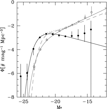
Binned representation of the shape of the late- and early-type LFs at 0.1 ≤z < 1.2, shifted to M* and φ* in redshift bin 2. Magnitude bins have been optimized one at a time. The thick solid curve represents the best-fitting Schechter function of early types and the thin curve of late types. Data points with error bars show the uncertainties on Φ in any one individual magnitude bin under the (idealized) assumption that all bins are independent. They serve as an upper limit on any deviation of the LF shape from the Schechter function, and show that the late-type LF does not exhibit a break down to at least Mr≈−14, but instead continues to rise steeply with α≥−1.65. The dotted line represents the sum of both LFs and the dashed line the steepest LF suggested by Blanton et al. (2005), which agrees well with ours around the onset of the faint-end upturn, although it fails to match our LF at the bright end.
The superposition of the shallow early-type and steep late-type LFs produces a distinct upturn at intermediate magnitudes of Mr≈−19. Such an upturn has been suggested by Blanton et al. (2005) on the basis of SDSS data. In the latter survey, the fairly shallow surface brightness limit prevents a direct measurement of the full faint end of the LF, but extrapolating for galaxies beyond this limit, their steepest estimate for the faint-end component is α=−1.52, slightly shallower than our result. This estimate is shown in Fig. 11 by a dashed line. Around the onset of the faint-end component, at Mr≈−19, our LF agrees very well in normalization and shape with the LF of Blanton et al. The Blanton LF does deviate significantly from ours at the bright end, a phenomenon already discussed in Section 4.5.
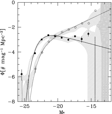
Binned representation of the shape of the late- and early-type LFs at 0.1 ≤z < 1.2, shifted to M* and Φ* in redshift bin 2. Here, all magnitude bins have been optimized simultaneously, representing our best estimate for the shape of the LF with associated uncertainties around the best fit. Shaded areas show how variations in the high- and low-redshift background LF parameters propagate into the best-fitting solution.
The principal conclusion from this figure is that we can constrain the late-type LF to Mr≈−14, and the early-type LF to Mr≈−15. A downturn in either LF above these magnitude limits can be ruled out. If mechanisms suppressing star formation do act to lower the abundance of dwarf galaxies from the extrapolated α≈−1.62 LF, this must happen at even fainter absolute magnitudes. There is some room for an excess of faint galaxies over the Schechter fits.
To gain a more accurate picture of the shape of the LF, we now carry out a simultaneous optimization of all magnitude bins of both SEDs. After finding the best-fitting solution, we obtain uncertainties with the previously described strategy (for each free parameter, we scan the range of values that yield an acceptable offset in χ2 from the best-fitting solution, allowing all other magnitude bins to be optimized in the background). The resulting LF is shown in Fig. 11. Error bars are again calculated for one degree of freedom and a confidence level of 68 per cent, as appropriate for an error calculation in a single parameter. The uncertainties are generally smaller than in the previous analysis, which at first appears counterintuitive (allowing the ‘uninteresting’ parameters to find a conditional maximum likelihood generally enlarges the uncertainties on any one ‘interesting’ parameter). However, this can be explained by the fact that we are now evaluating the uncertainties relative to the true maximum likelihood fit in the parameter space consisting of the individual magnitude bins, rather than the best Schechter fit.
This binned LF is sensitive to our assumptions for the values of the constant ‘background’ LF parameters at very low and very high redshifts. To illustrate this sensitivity, we have taken the output from the Monte Carlo trials discussed in Section 4.3 and calculated the binned LF for those trials not rejected due to their low likelihood. The shaded areas in Fig. 11 show the full range covered by these binned LFs.
The figure confirms the basic picture from Fig. 10: the late-type LF continues to rise steeply to Mr≈−14 without any indication of a break. Of all our Monte Carlo trial runs with acceptable likelihoods, not one exhibits a strong downturn in the faint-end slope at Mr < −14. Although the last two significant bins in the late-type LF do exhibit small, but significant deviations from the Schechter fit, the Monte Carlo results show that variations in the high- and low-redshift background can account for their magnitude.
The early-type LF is constrained well down to Mr=−16 and upper limits can be applied down to Mr=−14. These show that the LF follows our Schechter fit to at least Mr=−16. The uncertainties leave room for deviations from the power-law faint-end slope in either sense at fainter magnitudes, but none the less the late-type LF clearly dominates the total LF at least to Mr < −14.
We have repeated this analysis using the more stringent star/galaxy classifier limit of 0.8, instead of our default 0.97. This incurs the cost of possibly excluding very compact dwarf galaxies, but is closer to typical values adopted in the literature. As we have seen in Section 4.3, the best-fitting early-type LF is characterized by a slightly shallower faint-end slope and fainter M*, while the late-type LF is almost unaffected. However, calculation of the binned LF in the manner described above shows no qualitative difference in the shape of the LF, compared to our default calculation, which indicates that the recovered LF shape does not depend on the precise star/galaxy threshold (at least in the range 0.8 ≤S/G≤ 0.97, which is spanned by these two samples).
5 CONCLUSIONS
We have proposed a new Bayesian method for the calculation of galaxy LFs from multiband photometric samples. The method, the PML method, deconvolves the observed distribution of galaxies as a function of fluxes in multiple filter bands into the LFs of all galaxy populations (identified by redshift and SED type) that may contribute to this observed distribution. It thus eliminates the requirement to assign photometric redshifts to individual galaxies. This approach offers multiple advantages as follows.
The PML achieves a proper deconvolution of the observed data into the constituent galaxy populations.
The entire information contained in the multiband photometric data is retained for the calculation of the LF, instead of incurring the information loss that is associated with reducing these photometric data to a single best-fitting photometric redshift.
There is no requirement to model the often very complicated error functions of photometric redshifts; instead, only an understanding of the photometric error function is required.
Conventional photo-z determinations and LF calculations based on them are dependent on many (implicit or explicit) priors about the galaxy distribution as a function of redshift, which often go unacknowledged. By solving for the parameters of multiple galaxy populations over a large range of redshifts simultaneously, the PML significantly reduces the number of priors and allows for a self-consistent solution.
We have applied this algorithm to the E-CDFS field of MUSYC with the aim of recovering the faint-end shape of the LF at low redshift. For this purpose, we have represented the galaxy population up to z= 1.2 by two SED-specific Schechter functions (one for early- and one for late-type galaxies). Principal results are as follows.
In accordance with the current consensus in the literature, the LF of early-type galaxies is characterized by a fairly bright characteristic absolute magnitude M*r and a shallow faint-end slope, while the LF of late-type galaxies is much steeper.
The faint-end slope of the late-type galaxy population may be as steep as α≈−1.62. The superposition of these two SED-specific LFs produces an overall LF that cannot be described by a single Schechter function, but instead exhibits an upturn at intermediate magnitudes, where the late-type LF begins to dominate the overall LF. This upturn is noticeable in comparison to a standard α=−1.2 LF at magnitudes fainter than M≈M*+ 3 (M≈−19 in our sample).
The bright-end exponential cut-off is significantly brighter than found in the SDSS (Blanton et al. 2003), but slightly fainter than found in COMBO-17 (Wolf et al. 2003) from photometric redshifts.
We find fluctuations in the normalization of the LF and in the luminosity density with redshift in the E-CDFS that are broadly consistent with large-scale density inhomogeneities known from spectroscopic data but prohibit firm conclusions regarding any systematic trend of these quantities with redshift.
Calculation of the shape of the LF using a binned ansatz, rather than the analytical Schechter form, shows that the steep faint end extends at least as faint as Mr≈−14, which confirms the presence of a faint-end upturn. Therefore, we postulate a significantly larger number of dwarf galaxies in the Universe than would be predicted by simply extrapolating the typical faint-end slope of α≈−1.2 recovered in shallower field galaxy surveys to fainter magnitudes.
Our results show that, although our conclusions are qualitatively robust, statistical results still depend on priors, such as the extreme high-redshift LF, that are difficult to constrain in a self-consistent way, even with a high-quality data set such as MUSYC. Any work attempting to constrain these quantities from purely photometric data must give a careful account of the effect of such priors on its conclusions.
The PML formalism offers many opportunities for refinements. It can be easily generalized to calculate distribution functions over colours, stellar masses or star formation rates, as long as these quantities can be unambiguously assigned to the SED templates used in the analysis. To improve the calculation of LFs at high redshift, it is possible to implement passive redshift evolution in the SED templates, as opposed to the redshift-zero empirical templates which we have used in our analysis. We are planning a subsequent study of the full MUSYC catalogue which will explore some of these avenues.
DC gratefully acknowledges financial support from the Fundación Andes during the initial work on this project. DM is supported by NASA LTSA NNG04GE12G. EG is supported by the National Science Foundation under grant AST-0807570. We also acknowledge stimulating discussions with Edward Taylor and a helpful report from an anonymous referee that has greatly improved this manuscript.
REFERENCES
Appendix
APPENDIX A: MODIFICATIONS TO THE PUBLISHED MUSYC PHOTOMETRIC CATALOGUE
Adjustments to the photometric catalogue.
| Filter | Δ(mag) | e1 | e2 |
| U | −0.075 | 0.1 | 0.0 |
| B | +0.00 | 0.05 | 0.0 |
| V | +0.0125 | 0.04 | 0 |
| R | +0.025 | 0.03 | 0.0 |
| I | −0.1 | 0.08 | 0.4 |
| z | +0.075 | 0.09 | −0.4 |
| J | −0.15 | 0.15 | 0 |
| K | −0.075 | 0.2 | 0.0 |
| Filter | Δ(mag) | e1 | e2 |
| U | −0.075 | 0.1 | 0.0 |
| B | +0.00 | 0.05 | 0.0 |
| V | +0.0125 | 0.04 | 0 |
| R | +0.025 | 0.03 | 0.0 |
| I | −0.1 | 0.08 | 0.4 |
| z | +0.075 | 0.09 | −0.4 |
| J | −0.15 | 0.15 | 0 |
| K | −0.075 | 0.2 | 0.0 |
Parameters for corrections to the published photometric fluxes and uncertainties, according to equations (A1) and (A3).
The resulting relative zero-point shifts between any two optical filter bands are consistent with the numbers presented in Table A1, bolstering our confidence that the photometric residuals can indeed be predominantly ascribed to zero-point adjustments, rather than template insufficiencies. We do point out that we have not been able to use this method to independently verify our zero-point shifts for the J and K bands, because the number of objects permitting us to observe the same λrest through both filters at different redshifts is too small. However, the actual impact of these zero-point corrections on our LF results is minor and does not alter our qualitative conclusions.
The second adjustment to the photometric catalogue concerns the catalogue uncertainties. We have tested the catalogue MUSYC photometric uncertainties by comparing the scatter of the residual photometric fluxes from SED fitting to objects with known redshifts. While, in the ideal case, the residuals should show a Gaussian distribution (i.e. 68 per cent should fall within the published standard deviation, 95 per cent should fall within two standard deviations etc.), the residuals in the MUSYC catalogue typically exhibit a slightly larger scatter, indicating that the catalogue uncertainties are an underestimate and the scatter increases with an increasing flux. The latter behaviour is easily understood, because the published uncertainties only reflect internal photometric consistency, but do not include photometric calibration uncertainties or local background errors.
The effect of these two parameters e1 and e2 is to increase the uncertainties if they have been underestimated and to add a component to the uncertainty that is proportional to the flux (i.e. a zero-point calibration error). We have adjusted these two parameters manually for each filter band in order to achieve a more Gaussian-like distribution of the photometric residuals. The values are listed in Table A1.
