The evolution of star formation in quasar host galaxies Free

Abstract

1 INTRODUCTION

The interaction between the accretion process into a supermassive black hole residing at the centre of an active nucleus and star formation in the host galaxy is fundamental in regulating both galaxy evolution and the growth of the black hole. In order to understand the link between the two processes and assess the possibility of the two occurring concomitantly, it is important to quantify and constrain the star formation activity in quasar host galaxies. This is, however, a difficult task, as the star formation signature can be diluted by the strong active galactic nucleus (AGN) emission, especially at short [e.g. ultraviolet (UV)/optical] wavelengths. Emission emerging from star formation activity should, therefore, be looked for in the far-infrared (FIR), where the contribution of the AGN (in the form of thermal emission from dust) should be less important.

Combined AGN studies with IRAS and Infrared Space Observatory (ISO) already established the presence of strong FIR emission in quasars (see e.g. Verma et al. 2005 and references therein). According to some models, this radiation might be explained as the emission of dust distributed in a ‘cloud’ around the central engine with a 0.5-kpc radius (Siebenmorgen et al. 2004). However, other models estimate dusty tori extending to several kpc (e.g. Fritz, Franceschini & Hatziminaoglou 2006; Hatziminaoglou et al. 2008) with additional very large covering factors (≥90 per cent). Spitzer Infrared Spectrograph (IRS) spectroscopy revealed, in addition to the FIR emission, the presence of polycyclic aromatic hydrocarbon (PAH) features in the mid-IR spectra of optically selected quasars (Schweitzer et al. 2006) that are difficult to reproduce in models assuming dust heated by the hard AGN photons. A number of other arguments including the likely evaporation of PAH features in the presence of AGN emission and in the absence of high column densities (a necessary condition for the AGN to be able to heat the dust at such large distances) or the simultaneous presence of star formation evidence at other wavelengths suggest that the FIR in quasar host galaxies is more likely to be a tracer of star formation.

Even though Spitzer observations have increased the number of FIR detections in most low-redshift quasars (e.g. Schweitzer et al. 2006) and their analysis consistently points toward star formation driven FIR emission, the number of FIR detected quasars is still low. In preparation for the Herschel ATLAS (Astrophysical Terahertz Large Area Survey), an Open Time ∼500 deg² blank-field survey, and in preparation for targeted Herschel surveys of AGN, we need the best possible estimates for the quasar fluxes in Herschel bands. Most Sloan Digital Sky Survey (SDSS) quasars are not detected individually in the Spitzer Wide-Area Infrared Extragalactic (SWIRE) Legacy Survey 70- and 160-μm data (Londsdale et al. 2003, 2004) in the SWIRE–SDSS overlap region (e.g. Hatziminaoglou et al. 2005, 2008). Submm- and mm-wave observations of z≃ 2 and z > 4 quasars have yielded only a small number of direct detections (e.g. Omont et al. 1996, 2001, 2003; Carilli et al. 2001; Isaak et al. 2002; Priddey et al. 2003a,b; Robson et al. 2004; Beelen et al. 2006; Petric et al. 2006; Wang et al. 2007). IRAS and ISO detected just over half of the Palomar–Green (PG) quasar sample at 60 μm (e.g. Sanders et al. 1989; Haas et al. 2000; Haas et al. 2003).

In this paper, we will use stacking analyses to constrain the mean FIR luminosities of quasars, selected over a very wide range in redshift and absolute I-band magnitude. Our quasar compilation spans enough of the I-magnitude–redshift plane to be able to distinguish evolution from quasar luminosity dependence, which would be impossible in a single I-magnitude-limited quasar sample. Previous authors have stacked quasar fluxes at one (usually submm) wavelength, but we will combine a large body of multiwavelength FIR, submm- and mm-wave quasar photometry using an assumed common spectral energy distribution (SED). We will then show that our conclusions are robust to reasonable choices of SED. We follow SDSS in adopting the concordance cosmology of Ω_M= 0.3, Ω_Λ= 0.7, H₀= 70 km s⁻¹ Mpc⁻¹, and in assuming an optical spectral index of dln S_ν/dln ν=−0.5 for the quasars. In the FIR we assume an M82 SED shape from Efstathiou, Rowan-Robinson & Siebenmorgen (2000), unless otherwise stated.

2 METHODOLOGY

2.1 Sample selection

Fig. 1 shows the absolute I magnitudes of the SDSS quasars with SWIRE 70 and/or 160 μm coverage, against redshift. The SWIRE data were retrieved on 2007 August 17 and comprise version 2 products in the European Large Area ISO Survey (ELAIS) N1 and ELAIS N2 fields, and version 3 products in the Lockman Hole field. There are 281 Data Release 5 (DR5) SDSS quasars (Adelman-McCarthy et al. 2007) in the SWIRE fields with 70 and/or 160 μm coverage. Of these, 264 have 70 μm coverage and 261 have 160 μm coverage. ELAIS N1 is only partly covered by SDSS. There is no SDSS data for the Southern SWIRE fields XMM-LSS, ELAIS S1 or CDF-S, though this data were retrieved for calibration (see below); the version numbers are 2, 3 and 3, respectively. Fig. 1 also shows for comparison the PG sample with FIR photometry from IRAS and ISO (Sanders et al. 1989; Haas et al. 2000, 2003), in which non-detections have been remeasured using the scanpiIRAS fluxes discussed below. Fig. 1 also shows a compilation of the quasars observed at 850 and 1200 μm (Omont et al. 1996, 2001, 2003; Carilli et al. 2001; Isaak et al. 2002; Priddey et al. 2003a,b; Robson et al. 2004; Wang et al. 2007). The addition of the SDSS quasars to these data sets greatly improves the coverage of the optical luminosity–redshift plane. This will make it possible to make the first constraints on the evolution and luminosity dependence of star formation in quasar hosts. The right-hand panel of Fig. 1 demonstrates the FIR luminosities probed by the various multiwavelength data sets.

Figure 1

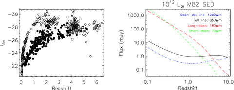
Left: absolute I magnitudes of quasars in this paper, as a function of redshift. Filled circles represent SDSS quasars with SWIRE coverage; open circles represent PG quasars with IRAS and B-band data; diamonds represent quasars observed at 850 μm; open squares represent quasars observed at 1200 μm (see text for details). Note that adding the SDSS quasars to the other samples greatly improves the coverage of the optical luminosity–redshift plane. Right: predictions for the FIR and submm fluxes of an M82 SED normalized to νL_ν= 10¹² L_⊙ at 100 μm. Note that the stacked signal from SDSS quasars at z≃ 2 are well matched in FIR luminosity to the expected stacked signal from PG quasars at z≃ 0.5.

Open in new tabDownload slide

2.2 SWIRE photometry

The SWIRE 70- and 160-μm images are supplied calibrated to surface brightness units of MJy sr⁻¹. We intend to measure the total mean point source flux of our targets, rather than the mean surface brightness at their locations, so we need to convert the units. We first note that a Gaussian point source with a peak flux of unity will have a total flux of F=πθ²_FWHM/(4 ln 2), where θ_FWHM is the full width at half-maximum (FWHM) of the point spread function. If θ_FWHM is measured in arcseconds, then this also gives the conversion between total point source flux and the flux per square arcsecond at the peak.

Using θ_FWHM= 1.22λ/D, where λ is the observed wavelength and D= 85 cm is the diameter of the telescope's primary mirror, we predicted the conversion between point source flux and surface brightness. This is shown in Table 1. We also derived an empirical conversion obtained by comparing the SWIRE point source catalogue fluxes with the background-subtracted map fluxes measured at the positions of the SWIRE sources. This comparison is shown in Fig. 2. The empirical conversion is some 29–36 per cent higher than the theoretical prediction, which may be due to the finite size of the map pixels, or a non-Gaussian shape to the point spread function shape (e.g. more resembling an Airy function). We adopt the empirical conversion in the analysis below.

Figure 2

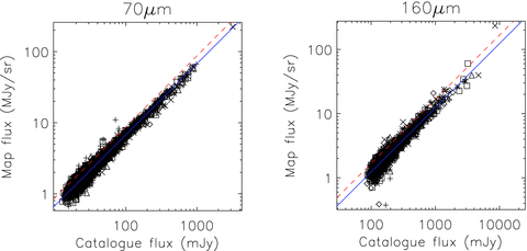
Conversion between map surface brightness units and point source total fluxes, using the SWIRE catalogues (not restricted to SWIRE quasars). The 70-μm data are shown to the left, and the 160-μm data to the right. The dashed (red) line shows the predicted conversion discussed in the text, and the full (blue) line gives the empirical conversion. Numerical values for the conversions are given in Table 1. Symbols: +– ELAIS N1, *– ELAIS N2, ⋄– CDFS, ▵– ELAIS S1, □– Lockman Hole, ×– XMM-LSS.

Open in new tabDownload slide

Although the maps are supplied with foreground DC offsets removed, we opted to subtract the mean flux level from each image. This ensures that the average total flux contribution is identically zero from each point source not associated with the SDSS quasars. The stacking methodology is to measure the point source fluxes from the SWIRE images at the positions of the SDSS quasars, and search for a significant deviation from zero flux. Photometric errors were estimated by measuring the standard deviation of the SWIRE images. The SDSS quasar astrometric errors are negligible compared to the SWIRE 70–160 μm beams.

2.3 IRAS photometry

scanpiIRAS flux estimates have recently been adapted to report negative AMP flux estimates, where acceptable fits are available. This would make this estimator suitable to stacking analyses, but we found positive fluxes on average reported at positions randomly offset from our targets (as noted also by e.g. Morel et al. 2001). This was found to be due to the scanpi algorithm allowing the source position to vary, so that the fits tended to gravitate to nearby noise features when the signal-to-noise ratio is very low. Therefore, we refit the co-added scanpi profiles allowing only the point source flux to vary, using the appropriate point source response function for the predominant scan direction (Alexov, private communication). We used the background-subtracted median co-added scans. At 60 μm, we subtracted an additional background estimate obtained by fitting a Gaussian to the off-source data histogram for each co-added scan (where ‘off-source’ is defined as where the template is <1 per cent of its maximum value). At 100 μm, the stronger baseline drifts visible in the co-added scans suggested a more local background subtraction. We defined the 100 μm on-source width to be where the template is >0.1 per cent of its maximum, and subtracted the mean of the co-added scan data in one template width either side of the target. Note that our flux calibrations discussed below were found to depend weakly on the sky subtraction algorithm, but were not independent of it.

We tested the flux calibration of stacked fluxes using 70-μm sources selected from the Spitzer legacy surveys SWIRE and Formation and Evolution of Planetary Systems (FEPS; e.g. Meyer et al. 2004; Hillenbrand et al. 2008), and using 90-μm sources selected from the ELAIS (Rowan-Robinson et al. 2004). Note that the SWIRE and ELAIS surveys were conducted in regions of low cirrus; the FEPS survey, while having fewer sources, is more widely distributed. We selected all SWIRE 70-μm sources in the flux range 12–300 mJy, then starting from the brightest, we rejected any source closer than 30 arcmin to any selected source. This ensured that both our source fluxes and their background estimates are statistically independent. We adopted the same selection procedure for ELAIS. For FEPS, we selected all sources with 70 μm detections at 5σ or above. For FEPS, SWIRE and ELAIS sources, we extracted IRAS fluxes in a 3 × 3 grid centred on the target, with grid positions separated by 20 arcmin.

To estimate the noise in each scanpi flux estimate, we tried two approaches: first, estimating the variance in the co-added scan from Gaussian fits to the data histogram, then propagating the noise in the best-fitting point source amplitude assuming the data points are statistically independent; secondly, measuring the variance of the point source amplitude estimates in the eight offset sky positions. The latter should give signal-to-noise ratio histograms with zero mean and unit variance, while for the former the histogram of (S_IRAS−S_Spitzer)/N_IRAS (where S and N are signal and noise, respectively) should also have zero mean and unit variance. The scanpi data points are not statistically independent, and we found that propagating the noise led to error estimates too small by a factor of around 3.6 at 60 μm, and 5.7 at 100 μm. The offset positions had consistent noise estimates, but have the disadvantage that the estimates are not local to the target. A visual inspection of the IRAS maps around our PG targets (Alexov, private communication) suggested problematic cirrus structure near several targets. We therefore adopted the propagated noise estimate, scaled by a factor of 3.7 (5.7) at 60 μm (100 μm) to account for correlations between the scanpi data points. Cirrus structure can in principle be alleviated with a matched filter tuned to the power spectrum of the background (e.g. Vio, Tenorio & Wamsteker 2002), though in this case the IRAS detector responsivity variations would present a significant complication.

We found the scanpi 1002 co-added scans (median combination of IRAS scans) to give the best signal-to-noise ratio. Figs 3 and 4 show the unweighted mean average IRAS fluxes of the fainter Spitzer and ISO sources in broad flux bins. This stacking methodology appears to give unbiased estimates even at the faintest 70-μm fluxes tested, e.g. ∼40 mJy at 70 μm. This is much fainter than the mean 60-μm fluxes of PG quasars, which we estimate to be 201 ± 35 mJy. For the offset positions, we estimated the signal and noise from a Gaussian fit to the histogram of the measurements, in order to avoid serendipitous sources. The stacked 60-μm fluxes at random offset positions were consistent with zero (e.g. 3.0 ± 1.5 mJy for SWIRE, see Fig. 3).

Figure 3

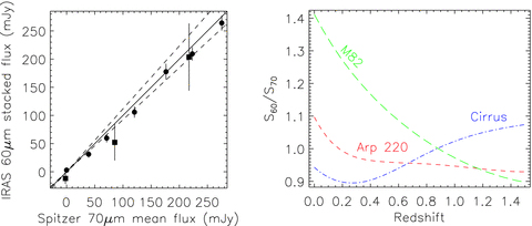
The left-hand panel shows the unweighted mean IRAS 60-μm AMP scanpi fluxes for Spitzer 70-μm SWIRE sources (circles) and FEPS sources (squares). The errors are the usual estimate of the noise on the mean, except for the zero-flux bins where the signal and noise are estimated from a Gaussian fit to the measurements as discussed in the text. The full line shows the 1:1 relation, and the dashed lines show the expected range of colours at 0.5 < z < 1.5 for M82, Arp 220 and a cirrus spectrum, from Efstathiou et al. (2000). Colours were calculated using the respective wavelength-dependent system responses, following the prescription in http://spider.ipac.caltech.edu/staff/lord/MIPS/MIPS.html. The redshift dependences of this colour for these SEDs are shown in the right-hand panel, with Arp 220 as short dashes, M82 as long dashes and cirrus as dash–dot.

Open in new tabDownload slide

Figure 4

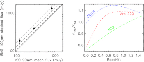
The left-hand panel shows the unweighted mean IRAS 100-μm stacked fluxes, as a function of ELAIS ISO 90-μm fluxes. Errors are as in Fig. 3. The dashed lines show the mean IRAS–ISO calibration offset found by Héraudeau et al. (2004), and the rms of their sample. The right-hand panel shows the expected IRAS–ISO colours expected for the SEDs as in Fig. 3.

Open in new tabDownload slide

At 100 μm, the stacked flux at blank-field positions offset from SWIRE sources was −6.7 ± 6.3 mJy. However, we found evidence for flux calibration discrepancy between ELAIS and our 100-μm stacked fluxes (Fig. 4). Héraudeau et al. (2004) found that the ELAIS 90-μm point source fluxes were lower than IRAS FSC 100-μm fluxes by a factor of 0.76 ± 0.17, after taking into account the colour corrections. They attributed this to systematic IRAS overestimates in the faintest catalogues fluxes, citing Moshir, Kopman & Conrow (1992); however, we find no evidence for such a calibration offset in our 60-μm IRAS stacks. We compared the ELAIS and SWIRE flux calibrations by interpolating the 70- and 160-μm fluxes to obtain 90-μm flux estimates, and found a 1:1 correlation with the ELAIS fluxes, so we think it unlikely the ELAIS flux calibration is at fault. We also calculated the 100 : 90 μm colour for our three SED models (Fig. 4), and found this too small an effect to account for the discrepancy. A similar discrepancy has been noted by Jeong et al. (2007), comparing IRAS 100-μm and AKARI 90-μm fluxes. We have therefore chosen to adopt the Héraudeau et al. correction factor of 0.76 to our stacked 100-μm IRAS fluxes. In Appendix A, we present our scanpi photometry of PG quasars and discuss the problematic cases.

3 RESULTS

3.1 Stacked flux results

Fig. 5 shows the SWIRE 70–160 μm fluxes for the SDSS quasars as a function of redshift and absolute magnitude. Error bars have been suppressed for clarity, except for a single representative example in each panel. The SDSS quasar population appears bimodal or at least with a significant skew to bright fluxes for a minority of objects, with a small number of FIR-loud objects at both 70 and 160 μm. For the bulk of the population, there also appears to be a significant positive flux at the positions of the SDSS quasars at redshifts z < 3, and at most absolute magnitudes. Of the quasars at 0.5 < z < 1.5, 6/114 have 70-μm fluxes above 20 mJy, and 6/113 have 160-μm fluxes above 70 mJy. In the 1.5 < z < 2.5 redshift bin, 3/86 have 70-μm fluxes above 20 mJy, and 3/84 have 160-μm fluxes above 70 mJy. The green curves show the predicted flux for an M82 SED, normalized to 10¹¹, 10¹² and 10¹³ L_⊙.

Figure 5

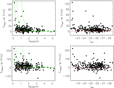
SWIRE 70- and 160-μm fluxes at the positions of SDSS quasars, as a function of the quasar absolute magnitudes and redshifts. A background sky level has been subtracted, as discussed in the text. The red line shows the prediction for zero flux, while the green curves show the location of an M82 starburst SED normalized to νL_ν= 10¹¹, 10¹² and 10¹³ L_⊙ at 100 μm. Note that at redshifts z < 3, and at most absolute magnitudes, the quasars appear significantly above the zero flux line. Error bars have been suppressed for clarity, except for a single representative error bar in each panel. Flux errors were estimated from Gaussian fits to the pixel histograms.

Open in new tabDownload slide

To test whether the skewed distribution is caused by a distinct population of FIR-loud quasars, or whether unrelated FIR-bright foreground companion galaxies are responsible, we compared the fluxes at the positions of SDSS quasars with those in the map as a whole, following the methodology of Serjeant et al. (2004). This test is preferable to Monte Carlo randomizations of the quasar positions, since it compares the quasar fluxes with the entire distribution of map fluxes, rather than a randomly selected subset. The results are shown in Fig. 6. The observed skewness in the quasar FIR fluxes is therefore not due to a pathological distribution of map fluxes. In Table 2, we present the average FIR fluxes for the SDSS quasars in redshift bins, both with and without the high-flux population.

Figure 6

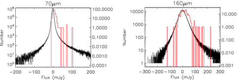
Histogram of map fluxes (fine bins, black line, left-hand ordinates) compared to the fluxes at the positions of the SDSS quasars (broad bins, red line, right-hand ordinates). Note the clear excess of positive fluxes at the positions of the SDSS quasars, i.e. the red lines are higher than the black lines on the right-hand sides.

Open in new tabDownload slide

It is clear from the curves in Fig. 5 that although the SDSS quasars span a narrow range of FIR fluxes, they span a wide range of FIR luminosities. The right-hand panel in Fig. 1 demonstrates that the stacked 160-μm signal from z≃ 2 quasars in SDSS covers comparable FIR luminosities to the expected stacked signal (a few times fainter than the IRAS PSC) from z≃ 0.5 PG quasars, for the assumed M82 SED. Furthermore, it is clear that combining the PG, SDSS and Submillimetre Common User Bolometer Array (SCUBA) quasars gives enough coverage of the optical luminosity–redshift plane to remove the degeneracy between trends in luminosity and in redshift (essentially Malmquist bias in its original sense; Malmquist 1924; see also Teerikorpi 1984).

3.2 Stacked luminosity results

It is not obvious what the best stacking statistic is where a large number of the sample have high signal-to-noise ratio direct detections, as is the case with our quasars. Variance weighting the stacks would result in high signal-to-noise ratio measurements dominating, but these measurements need not be in agreement with each other, because the population has an intrinsic dispersion. For example, if one has two quasars with fluxes 100 ± 1 and 0 ± 1 mJy, what can one say about the average in this population? Clearly, it would not be right to quote 50 ± 0.7 mJy for this average on the evidence of those two quasars.

We have opted to regard flux measurements of individual quasars as attempts to measure the mean of the population, so the dispersion in the population is a noise term on these measurements. The noise on any particular estimate of the population mean is therefore the quadrature sum of the flux error and the population dispersion.

However, what is an appropriate value for this population dispersion? We have opted to determine this from our data simultaneously with the population mean. If x_i are our measurements, each with a measurement noise level σ_i, then our data should have the following distribution:

1

where μ is the population mean and σ₀ is the population dispersion. We find the maximum likelihood solutions for μ and σ₀ from our data by maximizing Πρ(x_i, σ_i), and estimate the parameters' 68 per cent confidence bounds directly from the likelihood surface. Note that there is no covariance between these parameters; this follows from the fact that the expected values of measurements are independent of their noise levels. We used our estimated σ₀ values as noise terms to add in quadrature to our measurements, and calculated noise-weighted means. We used numerical simulations to verify that our estimators are unbiased.

This estimator worked well where we had more than three objects in a bin, but encountered numerical problems with some bins containing only two or three objects. There is also not enough information to constrain both parameters when there is only a single object. One option is to neglect the population dispersion σ₀ in these problematic cases, but this would lead to overoptimistic error estimates. Another option is to ignore these bins altogether. For readers that wish to do so, the numbers in each bin will be given. However, we found that the quantity in bins with >three objects ranged from 0.51 to 1.41, with a mean 0.84 and standard deviation 0.24. On this basis, we chose to adopt 0.84 as our estimator for σ₀ in bins with three or fewer objects.

We chose redshift and absolute magnitude bins and made a noise-weighted stack of the starburst FIR luminosities of the quasars in Fig. 1 in each of these bins, using the procedure above. FIR luminosities were estimated assuming an M82 SED. The results are listed in Table 3, and presented graphically in Figs 7 and 8. We will discuss the effects of varying the SED in Section 3.4. We used 160-μm fluxes as our FIR luminosity estimator for the SDSS quasars. For PG quasars we used the 60-μm fluxes at redshifts up to 0.3, and 100-μm fluxes at higher redshifts. Our results are not sensitive to the choice of z= 0.3 for this transition.

Figure 7

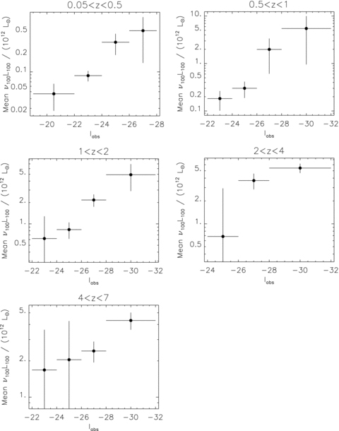
Optical luminosity dependence of the FIR luminosities of quasars, in five redshift slices, assuming an M82 SED template. Note that the FIR luminosities scale with the I-band luminosities, roughly as L_FIR∝L^0.5_opt.

Open in new tabDownload slide

Figure 8

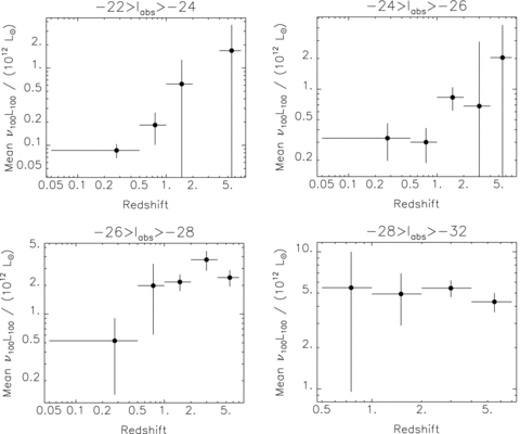
Evolution of quasar FIR luminosities in four absolute magnitude slices. Note the trends to brighter luminosities at higher redshifts, except in the brightest absolute magnitude strip. This can be interpreted as star formation in quasars decreasing with cosmic time, except perhaps in the most luminous quasars.

Open in new tabDownload slide

Taking bins in isolation, there are no high signal-to-noise ratio detections. Despite this, however, there are trends apparent in Figs 7 and 8. First, at all redshifts there appears to be a significant optical luminosity dependence, scaling as L^0.441±0.069_opt at z < 2 (see Fig. 7 and Table 4) and with a shallower scaling at higher redshifts. Secondly, at all absolute magnitudes below −28 and redshifts z < 2, there is a weaker signature of evolution (see Fig. 8 and Table 5). The poor χ² for the power-law evolution model in the −26 > I_abs > −28 bin is due to the highest redshift data point, in which the positive evolution is reversed, curiously mirroring the evolution of quasar number density. If this data point is excluded, the power-law fit parameters for this I_abs slice (Table 5) are ν₁₀₀L₁₀₀= (0.53 ± 0.25) × 10¹² L_⊙× (1 +z)^1.46±0.43, with χ²= 0.92 and Pr(χ², ν) = 0.37. This is consistent with the evolution at brighter absolute magnitudes, which justifies an estimate of the average evolution rate of I_abs > −28 quasars of (1 +z)^1.57±0.29.

3.3 Stacked black hole mass results

We next examined our data for trends with black hole mass. The black hole mass computation is based on the extrapolation of the reverberation mapping technique, which considers the velocity (FWHM) of emission lines and relates the size of the broad-line region (BLR) to the continuum luminosity. Assuming the dynamics of the BLR are dominated by the gravity of the black hole, the black hole mass is then expressed as

2

where R_BLR is the radius of the BLR and v is the velocity of the emission-line gas. The velocity v is estimated from the FWHM of Hβ, Mg ii or C iv depending on the redshift (Kapsi et al. 2000). For quasars with redshifts greater than z≃ 0.8, Hβ is not present in optical spectra, and Mg ii and C iv have been suggested as alternative estimators. For a detailed analysis of the method and the use of the various emission lines, see Kapsi et al. (2000), McLure & Dunlop (2004) and Warner et al. (2004). Depending on the redshift of the object and up to a redshift of 4.8, the following relations are used that have been argued by these authors to provide equivalent estimates:

3

4

5

where L_λ is the luminosity at wavelength λ. Black hole masses were estimated for objects with available SDSS DR5 spectroscopy. The FWHM of the lines were derived from the emission-line sigmas given by the SDSS pipeline, present in the second extension of the fits spectra. The error bars on the black hole masses are estimated from the uncertainty of the FWHM of the lines. We also searched the literature for additional black hole mass estimates. For PG quasars in Boroson & Green (1992), we recomputed the black hole masses using the relations above. For the z= 6.28 quasar SDSS J1148+5251, we applied equation (3) to the data in Shields et al. (2006). For other z > 5 quasars, black hole masses were taken from Jiang et al. (2007) and Kurk et al. (2007), using our equation (4) where possible, and equation (5) where only C iv is available. The black hole mass estimates vary between these two groups, even when using consistent conversions based on the same emission line, but because our mass bins are very broad (1 dex), these fractional variations (∼50 per cent) are not enough to move quasars to different bins. The results of the stacks in black hole mass and redshift bins are given in Table 6, and plotted in Figs 9 and 10. These figures give the host galaxy FIR luminosities as a function of black hole mass and of redshift. Tables 7 and 8 demonstrate the statistical significances of the trends in these figures.

Figure 9

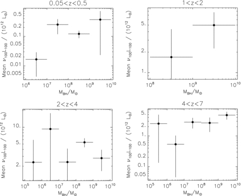
Host galaxy FIR luminosities as a function of black hole mass for selected bins in Table 6.

Open in new tabDownload slide

Figure 10

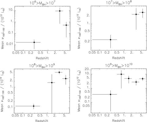
Host galaxy FIR luminosities as a function of redshift for selected bins in Table 6.

Open in new tabDownload slide

3.4 Robustness to SED assumptions

Any multiwavelength compilation such as this will inevitably rely on SED assumptions to relate the multiwavelength observations. We have assumed an M82 SED up to this point, and quoted FIR luminosities on that basis, but this will inevitably neglect any AGN dust tori contributions in the mid-IR. At best, our FIR luminosities can only be considered estimates of the starburst bolometric contributions. Starbursts, too, have a variety of SEDs, and in this section we will test the robustness to our assumed starburst SED shape. The most FIR-luminous quasars (i.e. those with direct SWIRE detections) were found by Hatziminaoglou et al. (2008) to resemble the heavily obscured starburst Arp 220 more often than M82, though they conjectured that fainter quasars would be more likely to resemble M82. We tested our SED dependence by rerunning our stacking analyses with an Arp 220 spectrum. Reassuringly, very similar trends are present as in the M82 case, perhaps because most of the rest-frame measurements are in spectral regions where the M82 and Arp 220 SEDs are similar (see Tables 9 and 10). Moreover, it would not appear to be possible to attribute the trends in Figs 7–10 to variations in SED shape as a function of quasar absolute magnitude, black hole mass or redshift.

Few objects in our compilation have photometry at more than one wavelength, except the SWIRE quasars. We tested our SED assumption by fitting M82 and Arp 220 SEDs to the SWIRE photometry. Of 236 quasars with photometric measurements at both 70 and 160 μm, 167 had χ² < 1 for either M82 or Arp 220 SEDs. Of these, 96/167 (57 per cent) had a lower χ² for M82. Since most of this photometry is non-detections, all this is capable of showing is that the underlying mean SED is more likely to resemble M82 than Arp 220, in agreement with the suggestion of Hatziminaoglou et al. (2008). Objects with χ² > 1 typically had evidence of a mid-IR excess, suggestive of an AGN dust torus.

We also tried estimating comparing the 70 : 160 μm flux ratio with the predictions for redshifted Arp 220 and M82 SEDs. The results are shown in Fig. 11. If an SED model is correct on average, the histogram in Fig. 11 should be centred around zero. This again suggests that an M82 SED is a better match to the average quasar FIR–submm SED than Arp 220 (though the most luminous may nevertheless more resemble Arp 220). This is in contrast with the bright quasars studied by Hatziminaoglou et al. (2008), though in keeping with their suggestion that fainter quasars have less heavily obscured SEDs. Note, however, that we have already excluded SED dependence on optical luminosity, redshift or black hole mass as explanations for the trends in Figs 7–10.

Figure 11

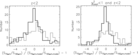
Comparison of the 70 : 160 μm flux ratio for SWIRE SDSS quasars (including individual SWIRE non-detections) for an M82 SED (thick histogram) and an Arp 220 SED (thin histogram). The left-hand panel is restricted to objects at redshifts z < 2, and the right-hand panel has the additional restriction that the best χ² of the M82 and Arp 220 models is better than 1. The x-axis shows the observed flux ratio divided by the predicted ratio, minus one. If the SED model choice is correct on average, the histogram should be centred on zero. The M82 histogram (thick) appears better centred on zero, so is favoured by this test.

Open in new tabDownload slide

4 DISCUSSIONS

4.1 Predictions for Herschel

Stacking analyses in general only yield information on the mean fluxes, and yield little information on the dispersion within the population. However, in the case considered here, we find evidence for a subset of quasars with bright FIR fluxes up to 10 times the mean fluxes within the population.

The 40 beams/source confusion limits predicted for Herschel by Rowan-Robinson (2001) are 4.6 mJy at 70 μm and 59 mJy at 160 μm. If we accept this estimate, then most of the targets in the AGN survey would therefore be very challenging for PACS direct detection. However, HSPOT reports a 5σ confusion limit of only 1.2 mJy at 110 μm, so this forecast may be pessimistic.

We used a crude fit to the data in Table 3 to predict the individual SDSS quasar fluxes (Figs 7 and 8), from which we estimate that the Herschel ATLAS survey will detect 92 per cent of SDSS quasars at z < 0.2 (though the z < 0.2 quasars represent only 0.5 per cent of all SDSS quasars). At higher redshifts, only the FIR-loud subset will be detectable. We estimate that 66 per cent of SDSS quasi-stellar objects (QSOs) with FIR luminosities five times larger than the mean will be detectable in this survey, corresponding to about 221(f₅/0.05) quasars detected over ≃500 deg², where f₅ is the fraction of quasars with luminosities five times larger than the mean. The detected fraction of five times overluminous quasars at z > 3 is only 5 per cent. However, the Herschel ATLAS survey should detect about 98 per cent of all the SDSS quasars with luminosities 10 times larger than the mean, i.e. about 333(f₁₀/0.05) quasars over 500 deg², where f₁₀ the fraction with luminosities 10 times larger than the mean.

We have neglected type 2 AGN in this analysis. These will double or triple the total number of AGN detected by the Herschel ATLAS survey. AGN not detected individually in this survey will be detectable in stacking analyses. It will be illuminating to test whether subclasses of quasars have a greater tendency to be FIR loud in this survey (e.g. broad absorption line quasars, nitrogen-rich quasars).

4.2 Physical interpretation

It might be possible for AGN dust tori models to account for the FIR and submm luminosities of quasars, but only by assuming very high equatorial optical depths and large physical sizes. If quasar heating dominated the FIR outputs throughout our sample, we would expect a linear correlation between quasar absolute magnitude and FIR luminosity (Fig. 7), whereas the observed correlation is shallower. While we cannot exclude AGN heating in a subset of our objects, we will follow Efstathiou & Rowan-Robinson (1995) in treating the FIR and submm luminosities of quasars as being typically dominated by star formation.

The FIR luminosities scale linearly with the star formation rates (SFRs) as

6

where L_FIR is the bolometric luminosity from the starburst (see Kennicutt 1998), assuming a Salpeter initial mass function (IMF) from 0.1 to 100 M_⊙, implying that our quasars are forming stars at around 200–2000 M_⊙ yr⁻¹. The local spheroid associated with a 10⁸(10⁹) M_⊙ black hole has a mass of about 5 × 10¹⁰ (5 × 10¹¹) M_⊙ (Marconi & Hunt 2003; Häring & Rix 2004), though there are indications that the spheroids are around a factor of 4 less massive at z= 2 (e.g. McLure et al. 2006). Sustained star formation at these rates could assemble the z= 0 stellar mass hosts in a few ×10⁷ to a few ×10⁹ yr.

The correlation between inferred black hole accretion and star formation is similar to the one reported by Hao et al. (2008), though they combined low luminosity–low redshift quasars with high luminosity–high redshift quasars, so their results could also have been attributable to evolution. We span a much bigger range of the optical luminosity–redshift parameter space (Fig. 1), so these caveats do not apply to our results.

The quasar magnitudes in our lowest redshift bin may in principle be contaminated by the host galaxies. If so, correcting for this effect would only strengthen the dependence of star formation on quasar luminosity, since the correction would apply preferentially at the faintest optical magnitudes.

One difficulty in the interpretation of these results is the possibility of luminosity-dependent reddening of quasars. However, even an A_V of one at the faintest end and zero at the brightest would have little impact on our correlations, given the size of our errors and range of absolute magnitudes. We have assumed a single optical spectral index for our quasars, but a slightly better approach would be to use the optical spectra themselves, correcting for dust absorption using the Balmer decrement where possible, or using rest-frame hard X-ray luminosities. Alexander et al. (2005) found an approximately linear relationship between hard X-ray and FIR luminosities in a heterogeneous sample of AGN-dominated submm-selected galaxies, though if one adds the submm galaxies classified as starbursts, their correlation is shallower with a wide dispersion. We have not excluded candidate starburst-dominated objects. Alexander et al. (2005) also demonstrate that local AGN show a large scatter in their star formation–black hole accretion relationship; our lowest redshift quasars in Fig. 7 show marginal evidence for a steeper correlation than at higher redshifts, broadly in agreement with these observations of local active galaxies.

The implicit correlations in Fig. 7 between SFR and black hole accretion rate hint at common physical parameters (such as gas supply), despite the disparity of spatial scales, but in keeping with qualitative expectations from the black hole–spheroid connections in local galaxies (e.g. Maggorian et al. 1998; Ferrarese & Merritt 2000). There is no insight to be gained by supposing the only common parameter is the total mass of the system, i.e. this is simply reflecting only a size dependence, because one must still hypothesize some mechanisms to tie both parameters to the total mass (e.g. Serjeant et al. 1998); in any case, the trends in Fig. 7 follow approximately L_FIR∝L^0.5_opt rather than a linear relationship. Furthermore, the lack of any obvious correlation with black hole mass at redshifts 0.5 < z < 4 (see below) argues against any simple scaling with the size of the system, at least outside the local Universe.

This non-linear relationship and its evolution do not follow expectations from some semi-analytic models. According to the model of Croton (2006), the ratio of black hole accretion rate and SFR is constant with scale but increases with redshift. This is partly due to increased disc disruption at high redshifts generating starbursts but not black hole accretion, and partly due to evolution in the black hole feeding rate in this model. The model does succeed in reproducing the evidence for evolution in the black hole–bulge mass relationships and (qualitatively at least) our evolving normalization of the black hole accretion–star formation relation from z < 0.5 to 1 < z < 2. However, it does not reproduce our scale dependence. Our observations may prove to be a useful constraint on AGN feedback models.

If AGN feedback directly regulates stellar mass assembly in the host, then we may expect stronger trends of FIR luminosity with black hole accretion than with black hole mass. Not all of our sample have black hole mass estimates, so our tests of dependence on black hole mass and redshift are more noisy than our correlations against quasar luminosity, though we span a larger logarithmic range of black hole mass than quasar luminosity. In the local Universe, we see a hint of a relation between SFR and black hole mass (Fig. 9, Table 7). At these lower redshifts, the hosts may already have assembled a large fraction of their z≃ 0 stellar masses, so this may partly represent mutual size dependence. However, at 0.5 < z < 4 there seems to be no evidence for a dependence on black hole mass (Fig. 9) despite the dependence on inferred black hole accretion (Fig. 7). At z > 4 there is some evidence for a weak trend with black hole mass (see Table 8), varying roughly as SFR ∝M^1/4_BH; the weakness of this trend suggests that it is less closely related to the primary underlying physical mechanism than the SFR–L_opt relation. There are nevertheless hints of trends with redshift at fixed black hole masses (Fig. 8, Tables 6 and 8). More black hole mass estimates are needed to improve the statistics, but our measurements are consistent with feedback from black hole accretion at z > 1 regulating the stellar mass assembly in their hosts.

It is likely that the e-folding time-scale for black hole growth [τ_BH≃ 4λ(0.1/ε) 10⁷ yr, where λ is the Eddington ratio and ε the accretion efficiency) is much faster than the stellar mass assembly time-scale (e.g. Malbon et al. 2007). Typical quasar lifetimes at z < 3.5 may not be much longer than a single e-folding scale (e.g. Martini & Weinberg 2001; Shen et al. 2007), though may be several e-foldings at higher redshifts (Shen et al. 2007). There are 3.6 e-foldings from I_AB=−22 to −26, making it unlikely that the relationships in Fig. 7 represent the evolutionary tracks of individual objects.

We have shown that active nuclei are on average associated with luminous or ultraluminous starbursts at all redshifts, and all absolute magnitudes brighter than about I_AB=−22. This relationship does not on its own help us address whether the AGN initiates the starburst or is started concurrently, or whether the AGN occurs at some mid-way point, or whether the AGN quenches the starburst. However, if quasar lifetimes are as long as 600 Myr at z > 3.5, which is the upper limit to the lifetimes suggested by Shen et al. (2007), then we would expect AGN feedback to have quenched the star formation in nearly all z > 3.5 quasars. Our tentative high-z detections suggest this is not the case. The high-z constraints will shortly be made much stronger with the large FIR and submm photometric surveys of z > 3.5 quasars from the Herschel ATLAS key project, SCUBA-2 and other facilities. Conversely, the shorter inferred quasar lifetimes at lower redshifts, the lack of evidence for any dependence of star formation on black hole mass, the observed dependence of SFR with quasar luminosity and the local bulge–black hole relationships are all consistent with feedback from black hole accretion regulating stellar mass assembly at lower redshifts.

This research has made use of the NASA/IPAC Infrared Science Archive and the NASA/IPAC Extragalactic Database (NED), which are operated by the Jet Propulsion Laboratory, California Institute of Technology, under contract with the National Aeronautics and Space Administration. We would particularly like to thank Anastasia Alexov, John C. Good and Anastasia Laity at IPAC for their invaluable help with the IRAS archive. We would also like to thank the anonymous referee for several helpful suggestions. This research was supported by STFC grants PP/D002400/1 and PP/E001408.

REFERENCES

Appendix

APPENDIX A: DISCUSSION OF PALOMAR–GREEN QUASARS

We use our scanpi 100-μm measurements in preference to other IRAS 100-μm measurements (e.g. Sanders et al. 1989), but that withstanding, we use the 100-μm photometry with the smallest errors with the exceptions of the cases discussed below. At 60 μm we use the measurements with the smallest errors regardless of their source, again with the exceptions discussed below. Haas et al. (2000), Haas et al. (2003) do not quote errors on their ISO photometry, but state that the detections range from 3 to 10σ. We conservatively assume 3σ unless stated otherwise. Objects dominated by non-thermal emission at 60–100 μm have been eliminated from our stacking analyses. The adopted photometry for the PG sample is given in Table A1.