A kinetic approach to cosmic-ray-induced streaming instability at supernova shocks Free

Abstract

1 INTRODUCTION

The problem of magnetic field amplification at shocks is central to the investigation of cosmic ray acceleration in supernova remnants (SNRs). The level of scattering provided by the interstellar medium turbulent magnetic field is insufficient to account for cosmic rays with energy above a few GeV, so that magnetic field amplification and large scattering rates are required if energies around the knee are to be reached. The chief mechanism which may be responsible for such fields is the excitation of streaming instabilities (SI) by the same particles which are being accelerated (Skilling 1975; Bell 1978; Lagage & Cesarsky 1983a,b). The effect of magnetic field amplification on the maximum energy reachable at SNR shocks was investigated by Lagage & Cesarsky (1983a,b), who reached the conclusion that cosmic rays could be accelerated up to energies of the order of ∼10⁴–10⁵ GeV at the beginning of the Sedov phase. This conclusion was primarily based on the assumption of the Bohm diffusion and a saturation level for the induced turbulent field δB/B∼ 1. On the other hand, recent observations of the X-ray surface brightness of the rims of SNRs have shown that δB/B∼ 100–1000 (see Völk, Berezhko & Ksenofontov 2005 for a review of results), thereby renewing the interest in the mechanism of the magnetic field amplification and in establishing its saturation level. It is, however, worth recalling that the interpretation of the X-ray observations is not yet unique: the narrow rims observed in the X-ray synchrotron emission could be due to the damping of the downstream magnetic field (Pohl, Yan & Lazarian 2005) rather than to severe synchrotron losses of very high energy electrons, although this interpretation has some serious shortcomings (see Morlino, Amato & Blasi 2008 for a discussion).

In this context of excitement, due to the implications of these discoveries for the origin of cosmic rays, Bell (2004) discussed the excitation of modes in a plasma treated in the magnetohydrodynamic (MHD) approximation and found that a new, purely growing, non-Alfvénic mode appears for high acceleration efficiencies. The author predicted a saturation of this SI at the level δB/B∼M_A(ηv_s/c)^1/2, where η is the cosmic ray pressure in units of the kinetic pressure ρv²_s, v_s is the shock speed and M_A=v_s/v_A is the Alfvénic Mach number. For comparison, standard SI for resonant wave–particle interactions leads to expect δB/B∼M^1/2_Aη^1/2. For efficient acceleration η∼ 1, and typically for shocks in the interstellar medium, M_A∼ 10⁴. Therefore, Bell's mode leads to δB/B∼ 300–1000, while the standard SI gives δB/B∼ 30. It is also useful to note that the saturation level predicted by Bell (2004) is basically independent of the value of the background field, since δB²/8π∼ (1/2)(v_s/c)P_CR, where P_CR is the cosmic ray pressure at the shock surface.

The resonant and non-resonant modes have different properties in other respects as well. A key feature consists in the different wavelengths that are excited. The resonant mode with the maximum growth rate has wavenumber k such that kr_L,0= 1, where r_L,0 is the Larmor radius of the particles that dominate the cosmic ray number density at the shock, namely for typical spectra of astrophysical interest, the lowest energy cosmic rays at the shock. At the shock location, the minimum momentum is the injection momentum, while at larger distances from the shock, the minimum momentum is determined by the diffusion properties upstream and is higher than the injection momentum, since higher energy particles diffuse farther upstream. When the non-resonant mode exists, its maximum growth is found at kr_L,0≫ 1. There may potentially be many implications of this difference: the particle–wave interactions, which are responsible for magnetic field amplification, also result in particle scattering (diffusion). The diffusion properties for resonant and non-resonant interactions are, in general, different. The case of resonant interactions has been studied in the literature (e.g. Lagage & Cesarsky 1983a), at least for the situation δB/B≪ 1, but the diffusion coefficient for non-resonant interactions (in either the linear or the non-linear case) has not been calculated (see however Zirakashvili & Ptuskin 2008). The difference in wavelengths between the two modes, in addition to different scattering properties, also suggests that the damping will occur through different mechanisms.

The calculation of Bell (2004) has, however, raised some concerns due to the following three aspects: (i) the background plasma was treated in the MHD approximation, (ii) a specific choice was made for the current established in the upstream plasma to compensate for the cosmic ray (positive) current and (iii) the calculation was carried out in a reference frame at rest with the upstream plasma, where stationarity is, in general, not realized (although for small-scale perturbations, the approximation of stationarity may be sometimes justified.).

In this paper, we derive the dispersion relation of the waves in a purely kinetic approach and investigate different scenarios for the microphysics that determine the compensating current. We show that the fast-growing non-resonant mode appears when particle acceleration is very efficient, but whether it dominates over the well-known resonant interaction between particles and Alfvén modes depends on the parameters that characterize the shock front, its Mach number primarily.

Bell (2004) also investigated the development of the non-resonant modes by using numerical MHD simulations. His results have been recently confirmed by Zirakashvili, Ptuskin & Voelk (2008) with a similar approach. Niemiec et al. (2008) made the first attempt to investigate the development of the non-resonant modes by using Particle in Cell (PIC) simulations. In this latter case, the authors find that the non-resonant mode saturates at a much lower level than found by Bell (2004). However, as briefly discussed in Section 5, these simulations use a setup that makes them difficult to compare directly with Bell's results.

The paper is organized as follows. In Section 2, we derive the dispersion relation of the unstable modes within a kinetic approach and adopt two different scenarios for the compensation of the cosmic ray current, namely compensation due to the motion of the cold electrons alone (Section 2.1), and to the relative drift of protons and electrons (Section 2.2). In Section 3, we discuss the relative importance of the resonant and non-resonant modes depending on the physical parameters of the system; we also derive analytic approximations for the large (Section 3.1) and small (Section 3.2) wavenumber limits. Finally in Section 4, we study the different modes during the Sedov evolution of a ‘typical’ SNR and for different assumptions on the background magnetic field strength. We conclude in Section 5.

Throughout the paper, we use the expressions accelerated particles and cosmic rays as referring to the same concept.

2 THE KINETIC CALCULATION

In this section, we describe our kinetic calculation of the linear growth of waves excited by streaming cosmic rays upstream of a shock. This type of analysis is not suited for the computation of the saturation level of the instability, but it can be used to investigate the type of modes that may possibly grow to non-linear levels.

In the following, all calculations refer to the shock location and not to an arbitrary location in the plasma upstream of the shock. This is to say that the minimum momentum of the particles considered in our calculations is the injection momentum.

In the reference frame of the upstream plasma, the gas of cosmic rays moving with the shock appears as an ensemble of the particles streaming at super-Alfvénic speed. This situation is expected to lead to streaming instability, as was indeed demonstrated in several previous papers [see Krall & Trivelpiece (1973) for a technical discussion].

In the reference frame of the shock, cosmic rays are approximately stationary and roughly isotropic. The upstream background plasma moves with a velocity v_s towards the shock and is made of protons and electrons. The charge of cosmic rays, assumed to be all protons (positive charges), is compensated by processes which depend on the microphysics and need to be investigated accurately.

The x-axis, perpendicular to the shock surface, has been chosen to go from upstream infinity (x=−∞) to downstream infinity (x=+∞). Therefore, a cosine of the pitch angle μ=+1 corresponds to the particles moving from upstream towards the shock.

The dispersion relation of waves in this composite plasma, in the test-particle regime that we wish to investigate here, can be written as (Krall & Trivelpiece 1973)

1

where the index α runs over the particle species in the plasma, ω is the wave frequency corresponding to the wavenumber k and Ω_α is the relativistic gyrofrequency of the particles of type α, which in terms of the particle cyclotron frequency Ω*_α and Lorentz factor γ is Ω_α=Ω*_α/γ. For the background plasma and for any population of cold electrons, one has Ω_α≈Ω*_α.

The positive electric charge of the accelerated cosmic rays, assumed here to be all protons, with total number density N_CR, must be compensated by a suitable number of electrons in the upstream plasma. In the following sections, we discuss two different ways of compensating the cosmic ray current and charge. In the first calculation, we assume that there is a population of cold electrons which is at rest in the shock frame and drifts together with the cosmic rays. These electrons exactly cancel the positive charge of cosmic rays. This approach is similar to that of Zweibel (1979, 2003) and resembles more closely the assumptions of the MHD approach of Bell (2004). In the second calculation, we assume that the current of cosmic ray protons is compensated by the background electrons and protons flowing at different speeds. This approach is similar to that of Achterberg (1983).

2.1 Model A: cold electrons

Let n_i and n_e be the number density of ions (protons) and electrons in the background plasma upstream of the shock. In this section, we consider the case in which a population of cold electrons with density n_cold streams together with cosmic rays and compensates their charge. Therefore, n_e=n_i and n_cold=N_CR. In terms of distribution functions, the four components can be described as follows:

2

3

4

5

In the latter equation, which describes cosmic rays, g(p) is a function normalized so that ⁠. In the above expressions, the background ions and electrons have been assumed to be cold (zero temperature). Introducing the thermal distribution of these particles does not add, as a first approximation, any important information to the analysis of the stability of the modes. One should check, however, that damping does not play an appreciable role, especially for the modes with high k[see Everett et al. (in preparation)].

The contribution of the background plasma of electrons and protons to the right-hand side of equation (1) is easily calculated to be

6

Similarly, the cold electrons with density N_CR contribute a term

7

The calculation of the cosmic ray contribution is slightly more complex. In its most general form, it can be written as

8

The integral in the variable μ is now

9

where denotes the principal part of the integral and we have neglected ω with respect to Ω_i (low-frequency modes). Using Plemelj's formula for the first term, one obtains for the cosmic ray response

where we have introduced the minimum momentum p_min(k) =m_iΩ*_i/k, which comes from the condition that the second integral in equation (8) is non-vanishing only when |μ| ≤ 1, namely when

10

The physical meaning of p_min is that of minimum momentum of the protons that can have a resonant interaction with waves of given wavelength.

In the limit of low frequencies that we are interested in, ω+kv_s≪Ω*_i≪ |Ω*_e|, the contribution of the background plasma can be Taylor-expanded and the unity in the dispersion relation (displacement current) neglected. So, the dispersion relation reads as

11

where is the Alfvén speed, is the wave frequency in the reference frame of the upstream plasma, and we have introduced

12

13

One should note that the phase velocity of the waves in the plasma frame is ⁠, and we want to concentrate on waves which have a velocity much smaller than the fluid velocity v_s (which is supersonic), therefore ⁠. In this limit, and using the fact that I^±₁=±I⁺₁, one can write the dispersion relation as

14

This dispersion equation is the same as that found by Bell (2004) by treating the background plasma in a MHD approximation. Here, we have obtained equation (14) by assuming that the cosmic ray current and charge are compensated by a population of cold electrons moving with the cosmic rays, a setup which is equivalent to that of having the cosmic ray current of Bell (2004). At least within the context of this specific choice of the compensating current, treating the background plasma within the MHD approximation as done by Bell (2004) does not change the results. However, the question arises whether the resulting dispersion relation may be different for a different and equally reasonable choice of the compensating current. In order to investigate this issue, in the following section we study the case in which the cosmic ray current is compensated by assuming a slow drift between thermal ions and electrons. This approach more closely resembles the kinetic approach first put forward by Achterberg (1983). It is also important to stress that this recipe is the same used recently in the PIC simulations of Niemiec et al. (2008).

2.2 Model B: compensation by electron–proton relative drift motion

The approach described in this section is the one originally put forward by Achterberg (1983). We show that the dispersion relation is identical to that found in the previous section, provided that the density of cosmic rays is low enough as compared to the density of the gas in the background plasma.

Within this approach, the electric charge of cosmic rays (assumed to be all protons) is compensated by the charges of electrons and protons in the background plasma

15

and the total current induced in the background plasma by the presence of cosmic rays vanishes, namely

16

This condition can be realized by requiring that electrons and protons move with slightly different velocities, v_s and v_e, respectively. The small drift between the two species leads to a current, which compensates the cosmic ray current.

For a given cosmic ray number density N_CR, the contribution of accelerated particles to the dispersion relation does not change as compared to the previous model of current compensation. The main differences with respect to the case presented in the previous section are that there are no cold electrons, and that electrons and protons in the background plasma have different velocities and densities. The contribution of the background plasma to the dispersion relation is then

17

Now, introducing the frequencies and ⁠, and using equations (15) and (16), and again taking the low-frequency limit, we obtain

18

Now we note that

so that, after neglecting terms ⁠, the contribution of the background plasma to the dispersion relation becomes

19

It is easy to recognize that the first term is the same as the contribution of the background plasma in Model A, while the second term is equal to the contribution of the cold electrons in Model A. It follows that the two dispersion relations are identical up to linear terms in series of (N_CR/n_i) and start to differ at the order of ⁠.

At this point, it is worth pointing out that in the numerical PIC simulations of Niemiec et al. (2008), the compensating current is realized by assuming a drift between protons and electrons, exactly as discussed in this section. However, in order to be able to carry out the calculations, the authors are forced to adopt unrealistically large values of the ratio N_CR/n_i (for the most realistic cases, they use N_CR/n_i= 0.3), which, as discussed above, do not necessarily result in a dispersion relation with the same characteristics as that found above and derived by Bell (2004).

3 RESONANT AND NON-RESONANT MODES

In this section, we investigate the modes that result from the dispersion relation in equation (14). For the sake of simplicity, we carry out our calculations for a power-law spectrum of accelerated particles with the canonical shape g(p) ∝p⁻⁴, which is expected from diffusive acceleration at strong shocks in the test-particle regime. This regime may potentially be different from the one relevant for particle acceleration in SNRs, in which acceleration takes place efficiently and the shock becomes cosmic ray modified by non-linear effects. The most evident effect of this non-linear reaction is the formation of a shock precursor which reflects in concave spectra of accelerated particles. The energy content of these accelerated particles is typically dominated by the highest energy particles, while numerically the low-energy particles are still dominant. On the other hand, efficient acceleration must proceed parallel to effective magnetic field amplification, and as showed by Caprioli et al. (2008a,b), the dynamical reaction of the strong field leads to a smoothening of the shock precursor, which in turn leads to the spectra of accelerated particles that, though still concave, are closer to power laws. It is straightforward to grasp the deeply non-linear nature of the problem at hand, where one is trying to describe the growth of waves associated with the cosmic ray streaming, but the latter only occurs after the waves have grown to interesting levels, so as to guarantee efficient particle acceleration. At the present time, a full analysis of the whole problem is simply not achievable. In the following, we still adopt the assumption of power-law spectra of accelerated particles, and we point out, where necessary, if a result may be substantially modified by non-linear effects.

The suitably normalized distribution function g(p) is

20

where Θ is the step function and takes into account the limited range of momenta spanned by the cosmic ray particles in the acceleration region.

The momentum p₀ is the minimum momentum of accelerated particles at the shock location, namely the injection momentum. Below, we discuss in detail the dependence of our results on the choice of the value of p₀.

Let us now consider the integrals I₁ and I₂ in equations (12) and (13). We integrate by parts after performing the substitution

21

obtaining

22

23

After defining s₀=kr_L,0 and s₂=kr_L,0p_max/p₀ and using the expression for g(s) obtained from equation (20) one finds

24

25

with s₁= Max [1, s₀]. Finally,

26

27

In terms of the latter, the imaginary and real parts of the frequency can be written as

28

29

where ⁠. It is useful to express α as a function of the acceleration efficiency of the shock. The total pressure in the form of accelerated particles is

30

The second part of this expression is a consequence of the fact that for spectra harder than p⁻⁵ and not harder than p⁻⁴, which are of interest here, the pressure is mainly contributed by relativistic particles with p∼m_ic. In case of cosmic-ray-modified shocks, spectra can become mildly harder than p⁻⁴, but this is not expected to affect our conclusion in a dramatic way, since it only introduces a weak dependence on p_max. Moreover, in case of strongly modified shocks, the major complication does not come from the spectrum of accelerated particles, but rather from the fact that the upstream plasma develops a precursor, namely a gradient in the fluid velocity that makes the standard treatment illustrated here formally not applicable. On the other hand, as pointed out several times throughout the paper, the magnetic reaction of the shock acts in the direction of smoothening the precursor, so that although formally the mathematical treatment illustrated here is not applicable, in practice it should provide a good description of the physical processes at work.

If we define η=P_c/(n_im_iv²_s) as the acceleration efficiency, we can write

31

where and r_L,0=p₀c/eB₀ is the Larmor radius of the particles with momentum p₀ in the background magnetic field B₀. We have also introduced ⁠. A resonant mode can be obtained from equation (28) with both signs of the polarization. On the other hand, the non-resonant mode appears only when the lower sign is chosen.

We note that the following relation holds

32

where J= e N_CRv_S. This means that the system is strongly current driven when ⁠.

Therefore, the parameter σ/v²_A controls the growth rate of the non-resonant mode: when σ/v²_A≫ 1, the non-resonant mode is almost purely growing and its growth is very fast. When σ/v²_A≪ 1, the non-resonant mode is subdominant and a resonant mode is obtained, asymptotically identical to that corresponding to the left-hand-polarized waves (upper sign in equation 28).

In the following, we often refer to the mode arising with the lower sign of the polarization as the non-resonant mode, although one should keep in mind that its peak growth rate reduces to that of the standard resonant mode in the limit σ/v²_A≪ 1.

In Fig. 1, we plot the solution of the dispersion relation in a case for which σ/v²_A≫ 1. The values of the parameters are v_S= 10⁹ cm s⁻¹, B₀= 1 μ G, n_i= 1 cm⁻³, η= 0.1 and p_max= 10⁵m_pc. The frequency (y-axis) has been normalized to the advection time for a fluid element upstream of the shock through the characteristic distance cr_L,0/v_S, namely cr_L,0/v²_S. It is worth stressing, however, that this is a good estimate of the diffusion time-scale only in the case of Bohm diffusion, when the diffusion coefficient is D(p) ≈r_L,0c and the diffusion time-scale is D(p)/v_S≈cr_L,0/v²_S. The plots in the upper (lower) panel in Fig. 1 are obtained by choosing the lower (upper) sign of the polarization in the dispersion relation (equations 28 and 29).

Figure 1

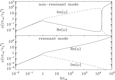
We plot the real and imaginary parts of the frequency as a function of wavenumber for the resonant and non-resonant modes. Wavenumbers are in units of 1/r_L,0, while frequencies are in units of v²_S/(cr_L,0). Top panel refers to the non-resonant branch, while lower panel is for the resonant branch. In each panel, the solid (dashed) curve represents the real (imaginary) part of the frequency. The values of the parameters are as follows: v_S= 10⁹ cm s⁻¹, B₀= 1 μG, n_i= 1 cm⁻³, η= 0.1 and p_max= 10⁵m_pc.

Open in new tabDownload slide

First, let us comment on the consistency of our derivation of the dispersion relation. It is easy to check, from Fig. 1, that these are indeed low-frequency modes. More specifically, they satisfy both assumptions underlying our calculation: and ⁠. Moreover, the non-resonant mode (lower sign of the polarization in the dispersion relation) is characterized by an imaginary part that is much larger than its oscillatory part for a very large range of wavenumbers. In this same range of k, for our choice of the parameters, its growth is much faster than for the resonant branch.

Further insight in the behaviour of the different wave modes can be gained by investigating the limits of the dispersion relation for the regimes kr_L,0≪ 1 and kr_L,0≫ 1. Based on these asymptotic trends, it is easy to explain (see Section 3.3) why the normalized frequencies as the functions of the normalized wavenumber, kr_L,0, do not depend on the choice of the minimum momentum.

3.1 Large wavenumber limit: kr_L,0≫ 1

For kr_L,0≫ 1, one easily obtains that I₁(k) ≃−(1/3)/(kr_L,0)² and I₂(k) ≃−(π/4)/kr_L,0. In equation (28), there are three terms that determine the actual dependence of on wavenumber k, namely

In the range kr_L,0≫ 1, the third term is always subdominant. Moreover, we can identify two critical values of the wavenumber k, k₁ and k₂, such that for k≫k₁≫ 1/r_L,0, the first term dominates upon the third, and for k≫k₂, the first term also dominates upon the second term, which is linear in k. It is easy to find that

33

Similarly,

34

For k≪k₂, equation (28) gives

35

When the upper sign is chosen in the above equation, we obtain ⁠, while when the lower sign of the polarization is considered, one finds ⁠, namely the growth rate of the waves increases with k. This is the non-resonant branch found by Bell (2004). For this mode, increases with k up to k∼k₂ and in the range of wavenumbers between k₁ and k₂ is larger than for the resonant waves. The maximum growth rate is obtained for k∼k₂. In fact, for k≫k₂ one finds

36

which implies for both the resonant and the non-resonant modes.

The non-resonant mode disappears when k₁ becomes larger than k₂, which happens for

37

For the reference values of the parameters, the non-resonant mode grows faster than the resonant mode only for unreasonably low efficiencies of particle acceleration, as one may conclude by comparing equation (37) with η∼ 0.1–0.2 required for the association of cosmic rays to SNRs.

On the other hand, for shock velocity v_s= 10⁸ cm s⁻¹ and magnetic field B₀= 5 μG, one easily sees that the limit in equation (37) becomes η < 0.1. This implies that the resonant and the non-resonant modes compete during the history of a SNR, with the resonant mode prevailing during the stages in which the shock has slowed down appreciably. We will comment further on this point below.

We summarize the results of this section by giving the following useful approximations to the solution of the dispersion relation in the large wavenumber limit. For 1/r_L,0≪k₁≪k≪k₂, we have

38

For k₂≪k, we have

39

3.2 Small wavenumber limit: kr_L,0≪ 1

In the limit of perturbations with wavelength much larger than the gyroradius of the lowest energy particles in the cosmic ray spectrum, the results again depend on the ratio between v²_A and σ. As we have already mentioned, for most regions of the parameters space v²_A≪σ, to which case we limit our analysis here, while we defer a discussion of what happens for slow shocks to the next section.

For kr_L,0≪ 1, one has I₁(k) →− 1. Hence, in the limit v²_A≪σ, we find for both signs of polarization:

40

3.3 Dependence on the minimum momentum

The number density of accelerated particles at the shock depends on the minimum momentum p₀, which in practice is hard to know or to predict, since it is determined by details of the microphysics of the shock formation. It is therefore useful to address the issue of the dependence of our results from the assumed value of p₀.

Let us start from the non-resonant mode. For k r_L,0≫ 1, following equation (35), we have that for k≪k₂ and for k≫k₂. It follows that apparently the dependence on p₀ is severe. However, if the wavenumbers k are normalized to 1/r_L,0 and is normalized to the diffusion time-scale r_L,0c/v²_S, the resulting imaginary and real parts of the frequency are independent of the choice of p₀. In other words, the absolute value of the growth rate is affected by the choice of p₀, but the rate itself, which is regulated by the time available for the instability to grow, as measured by the time-scale r_L,0c/v²_S, is independent of the choice of p₀. Similar considerations can easily be repeated for the resonant mode and for the low-frequency regime of the non-resonant mode.

4 RESONANT AND NON-RESONANT MODES IN SNRs

We now study the relative importance of the resonant and non-resonant wave modes during the evolution of a SNR. We consider a remnant originating in a SN explosion with energy E_SN. Once the remnant has entered the Sedov phase, the shock velocity as a function of time t can be written as

41

As discussed in the previous section, the existence of the non-resonant mode depends on the ratio σ/v²_A, which can be written as a function of the age of the remnant as

42

This implies that during the evolution of a ‘typical’ SNR, Bell's instability, which requires σ/v²_A≥ 1, is likely to operate only at early times after the beginning of the Sedov phase. The non-resonant mode disappears when the remnant is a few 10⁴ yr old if it is expanding in a 1 μG magnetic field and 10 times faster (age about a few 10³ yr) if the background magnetic field is 10 times higher. At later times, the streaming cosmic rays will still amplify the field but only via the classical resonant mechanism. This is also clear from Fig. 2 where we plot the growth rate of the non-resonant mode as a function of age for the above-mentioned values of the magnetic field: B₀= 1 μG in the upper panel and B₀= 10 μG in the lower panel. From the plots in Fig. 2, where again the time-scale for wave growth is normalized to the fastest of the time-scales involved in the system dynamics, c r_L,0/v²_S, one immediately sees that at least the resonant mode of the streaming instability still grows efficiently after 10⁶ yr since the supernova explosion. The non-resonant mode, on the other hand, soon becomes subdominant. The non-resonant mode grows the fastest at k∼k₂/2, so that from equation (38) we can derive the maximum growth rate as

43

It is clear that, remarkably, Γ_max does not depend on the background magnetic field B₀. On the other hand, the wavenumber at which the growth is maximum does depend on B₀ (see equation 34). These trends are clearly seen from Fig. 3, where we plot the dependence of the maximum growth rate on time, Γ_max, and of the wavenumber for which this occurs for both the resonant and the non-resonant modes. The plot refers to the ‘typical’ SNR parameters considered above and the two mentioned values of the background magnetic field strength. In both this figure and Fig. 2, a 10 per cent particle acceleration efficiency was assumed, and kept constant during the evolution of the remnant. This latter assumption is definitely not very realistic, as can be demonstrated by using the non-linear theory of particle acceleration.

Figure 2

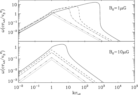
We plot the growth rate of the non-resonant mode as a function of wavenumber. Wavenumbers are in units of 1/r_L,0, while growth rates are in units of the advection time v²_S/cr_L,0. The different curves in each panel refer to different ages of the remnant: solid is for 10³ yr, dashed is for 5 × 10³, dot-dashed is for 10⁴, dot-dot-dashed is for 5 × 10⁴ and finally dotted is for 10⁶. Two different values of the background magnetic field strength are assumed in the two panels: B₀= 1 μG in the top panel and B₀= 10 μG in the bottom one. The shock velocity is computed according to the Sedov expansion of a remnant with E_SN= 10⁵¹ erg. The remaining parameters are as follows: n_i= 1 cm⁻³, η= 0.1 and p_max= 10⁵m_pc.

Open in new tabDownload slide

Figure 3

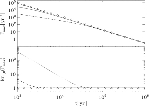
In the top panel, we plot the maximum growth rate of the resonant and non-resonant branches as a function of the age of the SNR. The growth rate is in units of yr⁻¹, while along the x-coordinate, time is expressed in yr. The notation for the different curves is as follows. The dashed line and the symbols are for the non-resonant mode in a 10 μG and 1 μG magnetic field, respectively; the solid and dot-dashed lines are for the growth of the resonant mode, again for B₀= 10 μG and B₀= 1 μG, respectively. In the bottom panel, we plot the wavenumber corresponding to the fastest growing wave mode for the same situations considered above. Wavenumbers are in units of r_L,0 and the notation for the different line-types is as follows. The dashed and dotted lines are for the non-resonant mode in a 10 and 1 μG magnetic field, respectively; the solid line and symbols are for the resonant mode, again for B₀= 10 and B₀= 1 μG, respectively. The shock velocity changes with time according to the Sedov evolution of a remnant with E_SN= 10⁵¹ erg. The remaining parameters are as follows: n_i= 1 cm⁻³, η= 0.1, p_max= 10⁵m_pc and p_inj= 10⁻²m_ic.

Open in new tabDownload slide

In Fig. 3, the time at which the fastest growing mode switches from non-resonant to resonant is identified by the intersection between the dashed line and the solid (B₀= 10 μG) or the dot-dashed (B₀= 1 μG) one depending on the magnetic field strength. The dominant wave mode progressively moves to larger wavelengths. The implications of this peculiar trend are expected to be profound on the determination of the diffusion coefficient: we recall that the standard Bohm diffusion is the limit obtained for resonant interactions of particles and waves, when δB(k) =B₀ for any value of k. For non-resonant modes, the diffusion properties need to be recalculated from first principles. On one hand, since the most unstable modes have k≫ 1/r_L,0, most particles do not resonate with these modes and the typical deflection suffered by a single particle within a spatial scale ∼1/k is very small. On the other hand, the number of scattering events is very large, therefore a substantial reduction of the diffusion coefficient can still be expected (see Reville et al. 2008; Zirakashvili & Ptuskin 2008).

5 CONCLUSIONS

We investigated the excitation of streaming instability induced by accelerated particles in the vicinity of a non-relativistic shock wave, typical of supernova shells expanding in the interstellar medium. The calculation is based on the kinetic theory, hence we do not require the MHD approximation to hold for the background plasma. We find that the dispersion relation of the waves leads to the appearance of the two modes, a resonant and a non-resonant one. The former is the well-known unstable mode, discussed by Zweibel (1979) and Achterberg (1983), based on a resonant interaction between waves and particles. The latter is similar to that discussed by Bell (2004), who however based his analysis on a set of assumptions that called for further investigation: the calculation of Bell (2004) is based on the assumption that the background plasma can be treated in the MHD regime, and makes specific prescriptions on the return current which compensates the cosmic ray current upstream of the shock. Moreover, the whole calculation is carried out in the frame of the upstream plasma, where, in principle, there is no stationary solution of the problem.

Our kinetic calculations are carried out for two models of the compensating current: in the first model, the return current is established through a population of cold electrons, at rest in the shock frame, which exactly compensate the positive charge of cosmic ray protons. In the second model, the return current is due to a slight drift between the ions and electrons in the background plasma upstream of the shock. We have demonstrated that the dispersion relation of the waves is the same in the two cases, of the order of ⁠.

The resonant and the non-resonant mode are found at the same time with growth rates, which in the general case are different. The non-resonant mode is almost purely growing and is very apparent when particle acceleration is efficient. The parameter that regulates the appearance of the non-resonant mode is σ/v²_A, where σ= 3ηv³_S/(c R). When σ/v²_A≫ 1, the waves excited in a non-resonant way grow faster than the resonant modes and may lead to a substantial magnetic field amplification.

The strong dependence of σ on the shock velocity implies that the non-resonant mode is likely to be the dominant channel of magnetic field amplification in SNRs in the free expansion phase and at the early stages of the Sedov–Taylor phase of adiabatic expansion. At later times, the non-resonant mode collapses on the resonant mode, which keeps providing appreciable growth for longer times, at least if damping mechanisms are neglected. The growth of the fastest non-resonant mode is independent of the strength of the unperturbed initial magnetic field B₀.

The non-resonant mode, when present, grows the fastest at wavenumber k₂ given by equation (34), which in the cases of interest is much larger than 1/r_L,0, where r_L,0 is the gyroradius of the particles with minimum momentum in the cosmic ray spectrum. These modes are therefore short wavelength waves, which is the main reason why the assumption of stationarity in the upstream frame, as required by Bell (2004), was acceptable, despite the impossibility of reaching the actual stationarity in that frame.

The numerical results in this paper were specialized to the case of a power-law spectrum p⁻⁴ of accelerated particles, typical of Fermi acceleration at strong shocks. However, one should keep in mind that the levels of efficiency required for the non-resonant mode to appear are such that the dynamical reaction of the accelerated particles on the shock cannot be neglected (see Malkov & O'C Drury 2001 for a review). This back reaction leads to several important effects: on one hand, the spectra of accelerated particles become concave and concentrate the bulk of the energy in the form of accelerated particles at the maximum momentum. On the other hand, the efficiently amplified magnetic field also exerts a strong dynamical reaction on the system, provided the magnetic pressure exceeds the gas pressure in the shock region (Caprioli et al. 2008a,b). This second effect results in an enhanced acceleration efficiency (due to large B-fields) but weaker shock modification (spectra closer to power laws) due to the reduced compressibility of the plasma in the presence of the amplified magnetic field. These non-linear effects cannot be taken into account in the type of calculations presented here, although we do not expect the qualitative character of our conclusions to be affected profoundly by them.

Nevertheless, it is useful to go through the possible consequences of the non-linear effects in a somewhat deeper detail: one can expect two types of complications, one of principle and the other in the numerical values of the growth rates. The latter simply derives from the approximations intrinsic in the assumptions we made: for instance, the adoption of a power-law spectrum of accelerated particles with slope 4, which clearly fails when a precursor is formed.

There are then complications coming from deeper unknown pieces of Physics or from a not-totally satisfactory mathematical approach. For instance, the standard perturbative approach adopted here is based on the assumption of a spatially uniform background. The presence of a precursor invalidates this assumption, although probably not in a dramatic way.

Since the non-resonant mode appears for large values of k, the relevant quantities can be assumed to be spatially constant in the precursor on scales ∼1/k, so that in this respect our calculations are still expected to hold, and probably to a better accuracy for the non-resonant modes (k≫ 1/r_L,0) than for the resonant ones (k∼ 1/r_L,0). Moreover, as stressed above, the dynamical reaction of the magnetic field leads to a weaker modification of the shock, and therefore to spectra with less prominent concavity (closer to p⁻⁴). Also in this respect, the calculations presented here should serve as a good description of all relevant physical effects related to the growth of the cosmic-ray-induced instabilities.

More importantly, the acceleration process is directly affected by the physics of particles' diffusion in the shock region, which in turn is determined by the excited waves. This intrinsic non-linearity cannot be taken into account in perturbative approaches like ours or like Bell's, and one should always be aware of this limitation. Even more, while the diffusion coefficient for resonant modes can at least be derived in the quasi-linear theory, at present there is no derivation of the diffusion coefficient associated with the scattering on non-resonant modes (see Zirakashvili & Ptuskin 2008 for a first attempt at discussing this effect).

Another issue that deserves further investigation is that of determining the level of field amplification at which the instability saturates. This cannot be worked out within a linear theory calculation and only numerical simulations can address this issue. Recent efforts in this direction have been made by Bell (2004) and Zirakashvili et al. (2008) through MHD simulations and by Niemiec et al. (2008) by using PIC simulations. While the first two papers find a saturation level δB²/(4π) ∼ (v_s/c)P_c, in the third paper a much lower level of the field amplification is found. The authors conclude that the existence of a large magnetic field amplification through the excitation of non-resonant modes is yet to be established.

Although we agree with this conclusion, we also think that the setup of the PIC simulation by Niemiec et al. (2008) is hardly applicable to investigate the excitation of the Bell instability at shocks, or at least several aspects of it should be studied more carefully. First, they carried out the calculations in a regime in which the condition of strong magnetization, ω≪Ω₀, was violated. Secondly, in order to carry out the calculations, Niemiec et al. (2008) are forced to assume unrealistically large values for the ratio N_CR/n_i (of the order of 0.3 for their most realistic runs). The return current as assumed by Niemiec et al. (2008) corresponds to our second model, which however leads to the same dispersion relation as Bell (2004) only at the order of ⁠, which is not necessarily the case here. Moreover, the spectrum of accelerated particles is assumed to be a delta-function at a Lorentz factor of 2, instead of a power-law (or more generally a broad) spectrum. It is not obvious that for non-resonant modes this assumption is reasonable. But the most serious limitation of this PIC simulation is in the fact that the authors do not provide a continuous replenishment of the cosmic ray current, which is instead depleted because of the coupling with waves. In the authors' view, this seems to be a positive aspect of their calculations, missed by other approaches, but in actuality the cosmic ray current is indeed expected to be stationary upstream, and we think that the PIC simulation would also show this if particles were allowed to be accelerated in the simulation box instead of being only advected and excite waves. Clearly, if this were done, the spectrum of accelerated particles would not keep its delta-function shape, but should rather turn into a power-law-like spectrum. The latter issue adds to the absence of a replenishment of the current, which seems to us to be the main shortcoming of these simulations. Overall, it appears that the setup adopted by Niemiec et al. (2008) would apply more easily to the propagation of cosmic rays rather than to the particle acceleration in the vicinity of a shock front.

The issue of efficient magnetic field amplification, possibly induced by cosmic rays, has become a subject of very active debate after the recent evidence of large magnetic fields in several shell-type SNRs. The implications of such fields for particle acceleration to the knee region, as well as for the explanation of the multifrequency observations of SNRs, are being investigated. Probably, the main source of uncertainty in addressing these issues is the role of damping of the excited waves. For resonant modes, ion-neutral damping and non-linear Landau damping have been studied in some detail: their role depends on the temperature of the upstream plasma and on the shock velocity. For non-resonant modes, being at high k, other damping channels could be important (Everett et al., in preparation). Whether SNRs can be the source of Galactic cosmic rays depends in a complex way on the interplay between magnetic field amplification, damping, particle scattering and acceleration, together with the evolution of the remnant itself.

The authors are very grateful to J. Everett and E. Zweibel for a critical reading of the manuscript and for ongoing collaboration and to B. Reville for constructive discussions. They also thank J. Kirk for identifying a problem in a previous version of the manuscript in the low-k part of the dispersion relation. This work was partially supported by the PRIN-MIUR 2006, by ASI through contract ASI-INAF I/088/06/0 and (for PB) by the US DOE and the NASA grant NAG5-10842. Fermilab is operated by the Fermi Research Alliance, LLC under contract number DE-AC02-07CH11359 with the US DOE.

REFERENCES