


Abstract
It has long been known that photoionization, whether by starlight or other sources, has difficulty in accounting for the observed spectra of the optical filaments that often surround central galaxies in large clusters. This paper builds on the first of this series in which we examined whether heating by energetic particles or dissipative magnetohydrodynamic (MHD) wave can account for the observations. The first paper focused on the molecular regions which produce strong H2 and CO lines. Here we extend the calculations to include atomic and low-ionization regions. Two major improvements to the previous calculations have been made. The model of the hydrogen atom, along with all elements of the H-like iso-electronic sequence, is now fully nl-resolved. This allows us to predict the hydrogen emission-line spectrum including excitation by suprathermal secondary electrons and thermal electrons or nuclei. We show how the predicted H i spectrum differs from the pure-recombination case. The second update is to the rates for H0–H2 inelastic collisions. We now use the values computed by Wrathmall et al. The rates are often much larger and allow the ro–vibrational H2 level populations to achieve a thermal distribution at substantially lower densities than previously thought.
We calculate the chemistry, ionization, temperature, gas pressure and emission-line spectrum for a wide range of gas densities and collisional heating rates. We assume that the filaments are magnetically confined. The gas is free to move along field lines so that the gas pressure is equal to that of the surrounding hot gas. A mix of clouds, some being dense and cold and others hot and tenuous, can exist. The observed spectrum will be the integrated emission from clouds with different densities and temperatures but the same pressure P/k=nT. We assume that the gas filling factor is given by a power law in density. The power-law index, the only free parameter in this theory, is set by matching the observed intensities of infrared H2 lines relative to optical H i lines. We conclude that the filaments are heated by ionizing particles, either conducted in from surrounding regions or produced in situ by processes related to MHD waves.
1 INTRODUCTION
The central galaxies in large clusters are frequently surrounded by a system of filaments that emit strong molecular, atomic and low-ionization emission lines. Understanding the origin of this line emission has been a long-standing challenge (Johnstone et al. 2007). The line luminosities are too great for the filaments to be powered by known sources of radiation such as the central active galactic nuclei or the diffuse emission from the surrounding hot gas. The evolutionary state of the gas is totally unknown. Two possibilities are that they form from surrounding hot gas or by ejection from the central galaxy in the cluster. Star formation may occur in the filaments although the emission-line spectra do not resemble those of Galactic H ii regions near early-type stars. Questions concerning the origin, energy source and evolutionary history are important, in part because of the large mass that may be involved, as high as ∼4 × 10¹⁰ M⊙ according to Salomé et al. (2006).
Infrared (IR) spectra show H2 lines which are far stronger relative to H i lines than those emitted by molecular gas near O stars. Attempts at reproducing the spectra assuming starlight photoionization are largely unsuccessful, as reviewed by Johnstone et al. (2007). Hybrid models, in which starlight produces the optical emission while other energy sources produce the molecular emission, appear necessary. The fact that optical and molecular emission luminosities trace one another (Jaffe, Bremer & Baker 2005) would require that these independent energy sources have correlated luminosities.
Since photoionization by O and B stars does not appear able to account for the spectrum, Paper I (Ferland et al. 2008) considered whether purely collisional heating sources can reproduce the observed spectrum. Magnetic fields occur in the environment and wave energy is likely to be associated with the field. Dissipation of this wave energy could heat the gas. Cosmic rays are also present (Sanders & Fabian 2007). These would heat and ionize the gas and produce strong low-ionization emission. Magnetohydrodynamic (MHD) waves may also accelerate low-energy cosmic rays within a filament. Similar particle and wave processes occur in stellar coronae where they are collectively referred to as non-radiative energy sources, a term we shall use in the remainder of this paper.
Paper I focused on H2 lines produced in molecular regions that are well shielded from light. Johnstone et al. (2007) detected H2 lines with a wide range of excitation potential and found a correlation between excitation and the derived population temperature. We found that non-radiative heating with a range of heating rates can reproduce the observed H2 spectrum. In this paper we concentrate on atomic and low-ionization emission and develop the methodology needed to predict the spectrum of gas with a range of densities but a single gas pressure. We find that cosmic ray heating produces a spectrum that is in general agreement with a wide range of observations. Purely thermalized energy injection cannot reproduce the spectrum. This does not rule out MHD wave heating but does require that they produce or accelerate high-energy particles in addition to other forms of energy. The resulting model, while empirical, points the way for a physical model of the origin of the filament emission.
2 SPECTRAL SIMULATIONS
2.1 The basic model
Starlight photoionization has long been known to have difficulty in reproducing observations of cluster filaments. Hybrid models, in which different energy sources produce the molecular and atomic emission are more successful but have problems accounting for why different energy sources would correlate with one another. Here we assume that only non-radiative heating, by either cosmic rays or dissipative MHD waves is important. The entire spectrum is produced by these energy sources.
For simplicity we assume that the gas is well shielded from significant sources of radiative heating. In reality light from the central galaxy or the surrounding hot gas will photoionize a thin skin on the surface of a cloud but will have little effect on the majority of the cloud's core. The emission lines emitted by the ionized layer will be faint. In the calculations that follow we include the metagalactic radiation background, including the cosmic microwave background (CMB), so that the continuum is fully defined from the gamma-ray through the radio. As described in Paper I this external continuum is extinguished by a cold neutral absorber with a column density of 1021 cm−2 to approximate the radiation field deep within the filaments. This continuum is faint enough to have little effect on the predictions in this paper.
In keeping with our assumption that the regions we model are well shielded, resonance lines such as the Lyman lines of H i or the Lyman–Werner electronic systems of H2 are assumed to be optically thick. Because of this continuum fluorescent excitation of H0 and H2 does not occur. With these assumptions the conditions in the cloud are mainly determined by the non-radiative heating sources which are the novel aspect of this paper.
For simplicity we assume that the chemical composition is the same as the local interstellar medium (ISM). The detailed gas-phase abundances are based on emission-line observations of the Orion star-forming environment and are given in Table 1. A Galactic dust-to-gas ratio is assumed. Refractory elements are depleted from the gas phase in keeping with our assumption that dust is present.
Assumed gas-phase abundances by log nucleon number density (cm−3) relative to hydrogen.
| He | −1.022 | Li | −10.268 | Be | −20.000 |
| B | −10.051 | C | −3.523 | N | −4.155 |
| O | −3.398 | F | −20.000 | Ne | −4.222 |
| Na | −6.523 | Mg | −5.523 | Al | −6.699 |
| Si | −5.398 | P | −6.796 | S | −5.000 |
| Cl | −7.000 | Ar | −5.523 | K | −7.959 |
| Ca | −7.699 | Sc | −20.000 | Ti | −9.237 |
| V | −10.000 | Cr | −8.000 | Mn | −7.638 |
| Fe | −5.523 | Co | −20.000 | Ni | −7.000 |
| Cu | −8.824 | Zn | −7.6990 |
Grains have several effects on the gas. H2 forms by catalytic reactions on grain surfaces in dusty environments. Collisions between gas and dust tend to bring them to the same temperature. This process either heats or cools the gas depending on whether the grain temperature is above or below the gas temperature. Molecules can condense as ices coating the grains if the dust becomes cold enough. Each of these processes is considered in detail in cloudy, the spectral synthesis code we use here, but the underlying grain theory depends on knowing the grain material, its size distribution, and the dust-to-gas ratio. The grain temperature depends on the ultraviolet (UV)–IR radiation field within the core, which in turn depends on whether in situ star formation has occurred. Rather than introduce all of these as additional free parameters we simply adopt the grain H2 catalysis rate measured in the Galactic ISM (Jura 1975). We do not consider grain–gas energy exchange and neglect condensations of molecules on to grain ices. Tests show that these assumptions mainly affect the details of the H0–H2 transition. One goal of this paper is to develop a physical model that accounts for the spectral observations. A long-term goal is to use such a model to determine the grain properties from observations of line extinction and the IR continuum.
Substantial uncertainties are introduced by the need to assume a specific gas-phase composition and dust properties. It would be surprising if the gas and dust composition happened to match that of the local ISM, although it would also be surprising if it were greatly different. The molecular collision rates, described in Section 2.4, have their own substantial uncertainties, probably 0.3 dex or more. These considerations suggest that there is roughly a factor of 2 uncertainty in the results we present below. This is intended as a ‘proof of concept’ calculation aimed at identifying what physical processes may power the observed emission. If successful, we can then invert the problem and determine the composition or evolutionary history from the spectrum.
2.2 Non-radiative energy sources
Paper I considered two cases, heating by dissipative MHD wave energy, which we assumed to be deposited as thermal energy, and cosmic rays, which both heat and ionize the gas. We refer to these as the ‘extra-heating’ and ‘cosmic ray’ cases below. The effects of these energy sources on the microphysics are fundamentally different.

We parametrize the extra-heating rate as the leading coefficient in the heating rate H0. We assume that the heating simply adds to the thermal energy of the gas so that the velocity distribution remains a Maxwellian with a well-defined kinetic temperature. With these assumptions the only collisional processes which occur are those which are energetically possible at the local gas kinetic temperature. This is a major distinction between the extra-heating case and the cosmic ray case described next.
The second case we consider is energy deposition by ionizing particles. These particles could be related to the high-energy particles which are known to exist in the hot gas surrounding the filaments (Sanders & Fabian 2007), or could be caused by MHD-related phenomena like magnetic reconnection (Lazarian 2005). Whatever their fundamental source we will refer to this as the cosmic ray case for simplicity. As in Paper I we specify the ionizing particle density in terms of the equivalent cosmic ray density relative to the Galactic background. We adopt the background cosmic ray H2 dissociation rate of 3 × 10⁻¹⁷ s−1 (Williams et al. 1998). Sanders & Fabian (2007) find an electron energy density that is roughly 103 times the Galactic background in inner regions of the Perseus cluster. This value guided our choice of the range of cosmic ray densities shown in the calculations which follow.
There is some evidence that this Galactic background cosmic ray H2 dissociation rate may be substantially too low. Shaw et al. (2008) found a cosmic ray ionization rate 40 times higher along the sightline to Zeta Per from detailed modelling while Indriolo et al. (2007) derived a value 10 times higher from the chemistry of H+3 along 14 different sightlines. If these newer, substantially higher, Galactic background rates are accepted as typical then the ratio of the cosmic ray rate to the Galactic background given below would be reduced by about an order of magnitude. This is clearly an area of active research (Dalgarno 2006). We adopt the Galactic cosmic ray background quoted in Paper I for consistency with that paper. We will express the particle ionization rate in terms of the Galactic cosmic ray background rate.
Cosmic rays both heat and ionize the emitting gas. Their interactions with low-density gas are described in Spitzer & Tomasko (1968), Ferland & Mushotzky (1984), Osterbrock & Ferland (2006), Xu & McCray (1991), Dalgarno, Yan & Liu (1999), Tine et al. (1997) and many more papers. Abel et al. (2005) describe our implementation of this physics in the current version of cloudy. Briefly, if the gas is ionized (the electron fraction ne/nH > 0.9) cosmic rays give most of their energy to free electrons which are then thermalized by elastic collisions with other electrons. In this highly ionized limit cosmic rays mainly heat the gas. In neutral gas, with low electron fraction, some of the cosmic ray energy goes into heating the gas but much goes into the creation of a population of suprathermal secondary electrons. These secondaries cause direct ionization as well as excitation of UV resonance lines. These excitation and ionization rates depend on the cosmic ray density and the electron fraction but not on the kinetic temperature of the thermal gas.
These two cases behave quite differently in the cold molecular limit and in the nature of the transition from the molecular to atomic and ionized states. In a cosmic ray energized gas the suprathermal secondary electrons will cause ionization and excite resonance lines even when the gas is quite cold. As the cosmic ray density is increased the transition from the fully molecular limit to the atomic or ionized states is gradual since the ionization rate, in the low electron-fraction limit, is proportional to the cosmic ray density and has little dependence on temperature. Thus a very cold cosmic ray energized gas will have a significant level of ionization, dissociation, and excitation of the H i, He i and H2 resonance transitions. The UV lines, being optically thick in a well-shielded medium, undergo multiple scatterings with most lines being absorbed by dust or gas. Some emission in IR and optical subordinate lines, and in ro–vibrational transitions in the ground electronic state of H2, occurs.
In the extra-heating case the thermal gas has a single kinetic temperature. As the extra-heating rate increases the temperature rises but the gas remains fully molecular until the kinetic temperature rises to the point where dissociation is energetically possible. The transition from molecular to atomic phase occurs abruptly when the gas kinetic temperature approaches the H2 dissociation energy. The gas will be in one of three distinct phases, with essentially all H in the form of H2, H0 or H+. As the heating rate and kinetic temperature increase the gas will go from one form to another in abrupt transitions which occur where the temperature reaches the appropriate value.
These two models mainly differ in how energy is deposited in molecular or atomic gas. The energy of a cosmic ray will eventually appear as heat, internal excitation or as an ionizing particle, while in the wave-heating case the energy deposition is purely as heat. The cosmic ray case does not exclude MHD effects as the fundamental energy source since MHD waves can produce low-energy cosmic rays within a filament (Lazarian 2005).
2.3 A fully l-resolved H-like iso-sequence
The calculations presented here use version C08.00 of the spectral synthesis code cloudy, last described by Ferland et al. (1998). There have been several improvements to the simulations since Paper I. These are described next.
The hydrogen recombination spectrum is special because it can be predicted with great precision. Two of the most important rates, radiative recombination and transition probabilities between bound levels, are known to a precision of several per cent. If the H i lines form by recombination in an ionized gas that is optically thick in the Lyman continuum then the emission-line spectrum should be close to Case B of Baker & Menzel (1938). Collisional excitation of excited levels from the ground state of H0 are a complication since their contribution to the observed H i spectrum depends on density, temperature and ionization in ways that are fundamentally different from the recombination Case B.
The computed H i emission-line spectrum presented here is the result of a full calculation of the formation of the lines, including radiative and three-body recombination, collisional ionization, collisional coupling between nl terms, and spontaneous and induced transitions between levels. For much of its history cloudy has used the compact model of the H-like iso-sequence described by Ferguson & Ferland (1997) with the rate formalism described by Ferland & Rees (1988). That model resolved the 2s and 2p levels but assumed that l-terms within higher n configurations were populated according to their statistical weights. This is formally correct only at high densities. Various approximations were introduced to allow the model to work well in the low-density limit.
Our treatment of the entire He-like iso-electronic sequence was recently enhanced to resolve any number of nl levels, resulting in a far better representation of the physics of the resulting emission. Applications to He i are discussed by Porter et al. (2005) while Porter & Ferland (2007) describe ions of the He-like sequence. This same methodology has now been applied to the H-like iso-sequence. Levels can now be fully l-resolved and any number can be considered. The methods used to calculate rates for l-changing collisions are given in Porter et al. (2005).
A very large number of levels, and resulting high precision, were used in Porter et al. (2005). This was possible because of the overall simplicity of that study. The temperature and electron density were specified so a single calculation of the level populations was sufficient to obtain the He i spectrum. The calculations presented below self-consistently solve for the temperature, ionization and chemistry, which requires that the model atom be re-evaluated a very large number of times for each point in the cloud. An intermediate model must be adopted with a small enough number of levels to make the problem solvable with today's computers but yet expandable to have more levels and become more accurate when more power becomes available or high precision is needed. A hybrid approach was chosen. The lowest n′ configurations are nl resolved. They are supplemented with another n′′ configurations, referred to as collapsed levels, which do not resolve the nl terms. The number of resolved and collapsed levels can be adjusted with a trade-off between accuracy and speed. In the following calculations levels n≤ 15 are nl resolved with another 10 collapsed levels representing higher states. This is sufficient to achieve a convergence accuracy of better than 2 per cent for the H i lines we predict. Larger errors are introduced by uncertainties in the collisional rates. These are difficult to quantify but probably produce errors of ∼20 per cent in the line emissivities and ∼5 per cent in relative intensities of H i lines.
Resolving the nl terms makes it possible to predict the detailed effects of thermal and cosmic ray excitation of optical and IR H i lines because the resulting emission spectrum is sensitive to the precise nl populations. High-energy particles will mainly excite np levels from the ground 1s term because most atoms are in the ground state and electric dipole allowed transitions have larger collisional excitation cross-sections at high energies (Spitzer & Tomasko 1968). After excitation, the np level will decay to a variety of lower s or d terms because of selection rules for optically allowed transitions. The H i Lyman lines are assumed to be optically thick so that np → 1s transitions scatter often enough to be degraded into Balmer lines plus Lα. The resulting Lα photons will largely be absorbed by grains rather than emerge from the cloud.
Quantal calculations of collisional excitation rates for excitation of nl terms by thermal electrons are used (Anderson et al. 2000). There is no favoured final l term, another distinction between the cosmic ray and extra-heating case. Details of the resulting optical and IR H i emission will be discussed below.
2.4 Revised H–H2 collision rates
The rates for collisions between H and H2 have been updated from those used in Shaw et al. (2005). We had used the fits given by Le Bourlot, Pineau des Forts & Flower (1999) in Paper I. Allers et al. (2005) noted that observations of H2 emission from the Orion Bar suggested that these rates were two small by nearly 2 dex. Wrathmall, Gusdorf & Flower (2007) confirmed this and presented a new set of collisional rate coefficients using an improved interaction potential and scattering theory. These rate coefficients for excited vibrational levels are systematically larger, often by 2–3 dex. These rates are employed in this paper.
 . If the total de-excitation rate (s−1) due to collisions with species S with density n(S) is
  , where qi,l is the collisional de-excitation rate coefficient (units cm3 s−1), then the critical density of a molecule in level i colliding with species S is given by
H2 lines, levels and critical densities at 1000 K.
| WL | ID | vup | Jup | Texc (K) | H0 | He | Ho2 | Hp2 | H+ |
| 28.21 | 0–0 S(0) | 0 | 2 | 509.8 | 1.11E+01 | 1.61E+00 | 3.76E+00 | 5.16E+00 | 2.36E−02 |
| 17.03 | 0–0 S(1) | 0 | 3 | 1015 | 1.54E+02 | 2.70E+01 | 6.18E+01 | 8.01E+01 | 4.14E−01 |
| 12.28 | 0–0 S(2) | 0 | 4 | 1681 | 7.49E+02 | 2.51E+02 | 5.17E+02 | 6.29E+02 | 1.52E+00 |
| 9.66 | 0–0 S(3) | 0 | 5 | 2504 | 2.40E+03 | 1.43E+03 | 2.91E+03 | 3.50E+03 | 5.96E+00 |
| 8.02 | 0–0 S(4) | 0 | 6 | 3474 | 6.37E+03 | 6.47E+03 | 1.28E+04 | 1.59E+04 | 1.27E+01 |
| 6.907 | 0–0 S(5) | 0 | 7 | 4586 | 1.51E+04 | 2.50E+04 | 4.45E+04 | 5.67E+04 | 3.02E+01 |
| 2.223 | 1–0 S(0) | 1 | 2 | 6471 | 4.78E+04 | 3.61E+04 | 9.14E+04 | 1.07E+05 | 2.76E+02 |
| 2.121 | 1–0 S(1) | 1 | 3 | 6951 | 3.60E+04 | 3.53E+04 | 8.52E+04 | 1.07E+05 | 2.57E+02 |
| 2.423 | 1–0 Q(3) | 1 | 3 | 6951 | 3.60E+04 | 3.53E+04 | 8.52E+04 | 1.07E+05 | 2.57E+02 |
| 2.033 | 1–0 S(2) | 1 | 4 | 7584 | 3.16E+04 | 5.53E+04 | 1.15E+05 | 1.39E+05 | 2.15E+02 |
| 1.957 | 1–0 S(3) | 1 | 5 | 8365 | 3.05E+04 | 6.77E+04 | 1.78E+05 | 2.10E+05 | 2.17E+02 |
| 1.891 | 1–0 S(4) | 1 | 6 | 9286 | 3.14E+04 | 1.25E+05 | 2.69E+05 | 3.21E+05 | 1.96E+02 |
| 2.248 | 2–1 S(1) | 2 | 3 | 12 550 | 1.84E+04 | 5.61E+04 | 1.25E+05 | 1.67E+05 | 3.19E+02 |
| 1.748 | 1–0 S(7) | 1 | 9 | 12 817 | 3.81E+04 | 4.44E+05 | 8.37E+05 | 1.04E+06 | 1.35E+02 |
There is likely to be a substantial uncertainty in all molecular collision rates. This is partially because molecular collisions are complicated many-body problems. The current H0–H2 rates, while sometimes substantially larger than the previously published set, do not yet include reactive channels (Wrathmall et al. 2007). The rates will become larger still, at temperatures where these reactions can occur, when this process is included.
These critical densities can give an indication of the density of the molecular gas (Jaffe, Bremer & van der Werf 2001). The distribution of level populations within H2 ro–vibrational levels can be determined from relative emission-line intensities. Jaffe et al. (2001) find that low v, J populations can be fitted as a single Boltzmann distribution corresponding to excitation temperatures ∼2000 K. In this paper we fit the observed H2 line intensities and do not present H2 level-excitation diagrams. The results are fully equivalent but have the simplification that we are working with the directly observed quantity.
A thermal population distribution will result if the gas density is greater than the critical densities of the levels involved. Jaffe et al. (2001) argue that the density in the filaments must be ≥106 cm−3 if the gas is predominantly molecular. They based this on a modified scaling of the Mandy & Martin (1993) semiclassical H2–H2 collision rates. The rate coefficients presented by Le Bourlot et al. (1999) would suggest a significantly higher density (≥109 cm−3). Paper I showed that there are other ways to establish a quasi-thermal distribution at fairly low densities. Table 2 shows that the well-observed 1–0 S(1) line at 2.121 μm has a critical density ranging from 3 × 102 cm−3, for collisions with H+, to 1.9 × 105 cm−3, for collisions with H2. In practice the critical density will depend on whether ions are mixed with the molecular gas. We show below that the extra-heating and cosmic ray cases have very different mixtures of molecules, atoms and ions, and this may provide a discriminant between the energy sources. Note that only collisions with H0 and H+ are capable of inducing a reactive ortho–para transition in H2 (Dalgarno, Black & Weisheit 1973).
2.5 Lα pumping of H2
Lα fluorescence can be a significant H2 excitation source when ions and molecules are mixed as discussed by Black & van Dishoeck (1987) and Lupu, France & McCandliss (2006). In effect H2 offers a second channel, competing with dust, to remove Lα photons created by collisional excitation and recombination. The Lα energy is converted into internal H2 excitation energy and eventually dissociation or H2 line emission.

3 THE DENSITY–HEATING PLANE
3.1 General considerations
The magnetic field and cosmic ray density within the filaments are not known. The gas density is low enough for the optical [S ii] lines to be near their low-density limit (Hatch et al. 2006), n < 103 cm−3, but the density of the molecular gas is only constrained from the form of the H2 level-population distribution (Jaffe et al. 2001). Given these uncertainties we explore a broad range of non-radiative heating rates and gas densities, compute the thermal and chemical state of the gas, and predict the resulting emission-line spectrum to compare with observations. Results are presented below as a series of contour diagrams showing various predictions.
The non-radiative energy sources are the dominant heating agents for most conditions shown here. For the very lowest values of the heating rates the background metagalactic radiation field, described above, becomes significant. The resulting emission will be unobservably faint in this limit, however, as shown in diagrams below and in Paper I.
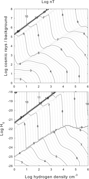
Fig. 1 shows the gas kinetic temperature, Fig. 2 shows the hydrogen molecular fraction, and Fig. 3 shows the fraction of H in H+. In all pairs of figures the upper and lower panels show the cosmic ray and extra-heating cases, respectively.

The log of the gas kinetic temperature is shown as a function of the hydrogen density, the independent variable and (top panel) the cosmic ray density relative to the Galactic background and (bottom panel) the leading term in the extra-heating rate. The temperature is near the CMB in the lower right-hand corner and rises along a diagonal from lower right-hand to upper left-hand side as the heating increases and the gas density decreases. There are discontinuous jumps in the temperature as the gas changes thermal phase.
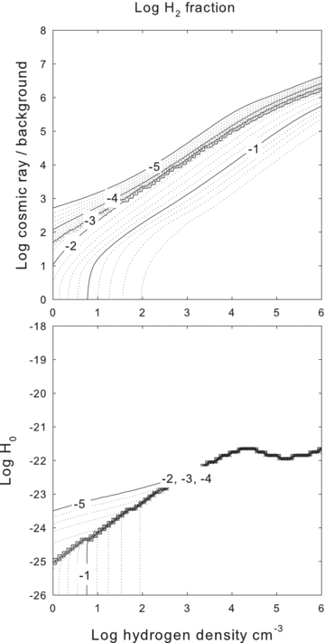
The log of the H2 fraction is shown as a function of the hydrogen density and (top panel) the cosmic ray and (bottom panel) the extra-heating rates. Gas is molecular in the lower right-hand corner where the density is high and the non-radiative heating rates are low. The gas is nearly fully molecular in the lower right-hand corner and becomes increasingly ionized along a diagonal running to the upper left-hand side. There are discontinuous jumps in the chemistry as the gas changes phases.
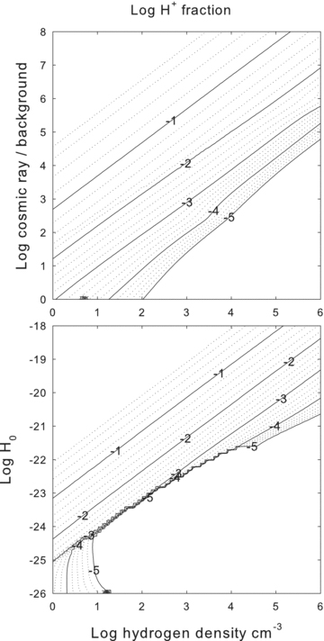
The log of the H+ fraction is shown as a function of the hydrogen density and (top) the cosmic ray and (bottom) the extra-heating cases. Gas is ionized in the upper left-hand corner of the diagram, where the density is low and the non-radiative heating rates are high, and molecular in the lower right-hand corner.
An ‘effective’ ionization parameter, given by the ratio of the non-radiative heating to the gas density unr=rnr/n(H), characterizes physical conditions in these environments. The non-radiative heating acts to heat and ionize the gas, while cooling and recombination processes are often two-body processes which increase with density. The ionization and temperature tend to increase with unr along a diagonal running from low heating and high density, the lower right-hand corner, to high heating and low density, the upper left-hand corner. The temperature and molecular fractions tend to change along diagonals from the lower left-hand to upper right-hand corners. These are along lines of roughly constant unr.
The lower right-hand and upper left-hand corners of the plane have the most extreme conditions. Gas is cold and molecular in the lower left-hand, high-density, low-heating corner. The kinetic temperature has fallen to nearly that of the CMB in this region. A small degree of ionization is maintained by background light or cosmic rays. This is to be contrasted with gas in the upper left-hand, high-heating, low-density corner. That gas is hot, with T≫ 104 K, and highly ionized. Gas in either region would emit little visible/IR light and so would be difficult to detect.
3.2 The H2 emission spectrum
Paper I described the H2 emission spectrum in some detail. Although the detailed predictions have changed due to the improved collisional rate coefficients used in this paper, the overall trends of H2 emission shown in that paper have remained the same.
The full H2 spectrum is presented below. Here we concentrate on the H2 0–0 S(2) λ12.28 μm line which we will combine with optical H i lines to set constraints on our simulations. The log of the emissivity 4πj (erg cm−3 s−1) of the H2 line is shown in Fig. 4. H2 emission occurs within regions where the H2 molecular fraction, shown in Fig. 2, is significant. Other factors besides the H2 density determine the line's brightness.
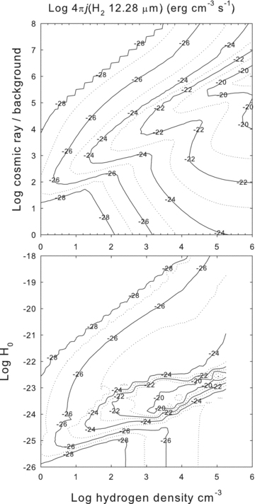
The log of the emissivity 4πj (erg cm−3 s−1) of the H2 0–0 S(2) 12.28 μm line is shown as a function of cloud parameters. This figure is to be contrasted with the next figure showing the H i line emissivity over a similar range of parameters.

The λ12.28 μm line is a pure rotational transition with an level excitation energy of 1681 K. The line is excited by two processes in our simulations. The line is emitted efficiently when the gas becomes warm enough for thermal particles to collisionally excite the upper level but not so warm as to dissociate the H2. This produces the region of peak emission that tracks the contour giving T∼ 2000 K in Fig. 1.
The H2 line remains emissive in much cooler regions in the cosmic ray case. Here suprathermal electrons excite the line by a two-step mechanism that is analogous to the Solomon process in starlight-excited PDRs (photodissociation regions). The first step is a suprathermal excitation from the ground electronic state X to one of the excited electronic states. A minority of these return to rotation–vibration levels within X. Many of these eventually decay to the upper level of the λ12.28 μm line. Other electronic excitations lead to dissociation which are then followed by formation by the grain surface or H− routes. These formation processes populate excited levels within X which then lead to emission. Details of our implementation of these H2 excitation processes are given in Shaw et al. (2005) and Shaw et al. (2008).
3.3 The H i emission spectrum
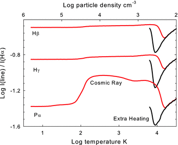
We consider the emissivity of Hβλ 4861Å in detail since we will use the H iλ4861 ÅH2λ12.28 μm line ratio to constrain our simulations. We also consider two H i line ratios that can be used to indicate whether the spectrum has been affected by interstellar reddening. This is important because the dust content of the filaments is currently unknown.
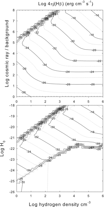
The log of the emissivity 4πj (erg cm−3 s−1) of Hβλ4861Å is shown as a function of cloud parameters. This figure is to be contrasted with those in Paper I which show the H2 line emissivity over a similar range of parameters.
H i lines can also form by collisional excitation in regions where H is mostly atomic. The gas must be warm enough to excite the upper levels of the optical or IR H i lines, requiring a temperature T≥ 4000 K, although collisional excitation is important at low temperatures in the cosmic ray case when suprathermal secondary electrons are present. The emissivity of a collisionally excited H i line is proportional to n(H0)nxf(T) where n(H0) is the atomic hydrogen density, mostly in the ground state, and nx is the density of the colliding species. The function f(T) is the Boltzmann factor of the upper level of the H i line for the case of excitation by thermal particles and is a constant for excitation by secondary electrons. Collisionally excited H i lines are emitted most efficiently by gas that is dense, atomic and warm.
The extra-heating case is relatively simple since only thermal processes affect the excitation and ionization of the gas. The lower panel of Fig. 5 shows that the line has a ridge of relatively high emissivity which corresponds to moderate ionization and temperature. The H i lines along this ridge are mainly produced by collisional excitation with a contribution from recombination following collisional ionization. The emission falls off dramatically when the gas becomes molecular in the lower right-hand corner or very hot in the upper left-hand corner.
Fig. 5 shows the Hβ emissivity in the cosmic ray case. Collisional excitation is also a dominant contributor to the line. The ridge of peak emission occurs for the same reason as in the extra-heating case. Significant H i emission occurs in the lower right-hand corner since the dissociative cosmic rays prevent the gas from becoming fully molecular even when it is quite cold. The population of secondary electrons produces a significant collisional excitation contribution to the H i lines across most of the lower right-hand half of Fig. 5.
In both heating cases the emissivity tends to rise along a diagonal from the lower left-hand to upper right-hand side. This corresponds to rising nenp at nearly constant T. This figure clearly indicates that powerful selection effects operate in this environment. As we show below, the emissivity of the H i lines is substantially higher than produced in the pure-recombination case due to the collisional contribution. This affects the use of H i lines as indicators or the gas of ionized gas.
The H i lines are often used to measure the amount of interstellar extinction. It is unusual for the H i recombination spectrum to deviate very far from Case B for moderate densities and optical depths in the Lyman continuum in a photoionized cloud (Osterbrock & Ferland 2006). This is because the relative H i line intensities are mainly determined by the transition probabilities. These determine which lines are emitted as the electrons cascade to ground after capture from the continuum. The result is that the spectrum depends mainly on atomic constants and less so on the physical conditions in the gas.
The ratio of the intensity of Hαλ6563Å relative to Hβλ4861Å, two of the strongest lines in the optical spectrum and a possible reddening indicator, is shown in Fig. 6. The Hα/Hβ intensity ratio is ∼2.8 for Case B in low-density photoionized gas (Osterbrock & Ferland 2006). The predicted ratio is significantly larger than this in most regions where the H i lines have a large emissivity.
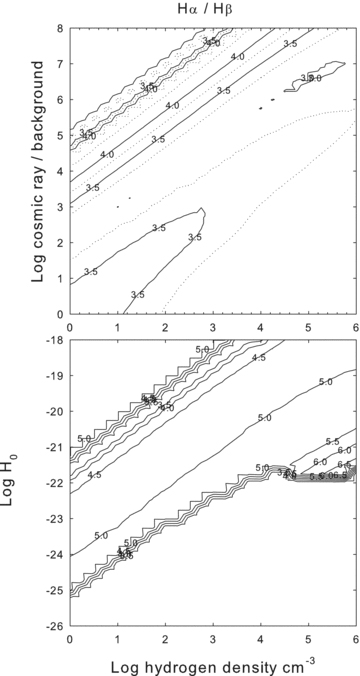
The ratio of emissivities of H iHαλ6563 to Hβλ4861 is shown as a function of cloud parameters. The ratio is ∼2.8 under the Case B conditions expected for photoionized nebulae. It is significantly larger for most parameters shown here because of collisional contributions to the line.
It is possible to measure intensities of H i lines that originate in a common upper atomic level with spectra that cover both the optical and IR. The Pαλ1.87 μm and Hβλ4861Å lines, with a common n= 4 upper configuration, is an example. Each of these lines is actually a multiplet with 4 nl terms within the upper level. At conventional spectroscopic resolution the lines within the multiplet appears as a single H i line. The transition probability of this multiplet depends on the distribution of nl populations with the upper terms, which in turn depend on the gas density (Pengelly 1964). Such line ratios are not expected to depend on the physical conditions as much as lines that originate in different configurations.
Fig. 7 shows the computed Pαλ1.87 μm/Hβλ4861Å intensity ratio. It is not constant because of the changing populations of nl terms within the n= 4 configuration of H0. At high densities the l terms will be populated according to their statistical weight and the level populations are said to be well l-mixed. The line intensity ratio is then a constant that is determined by the ratio of transition probabilities and photon energies. cloudy treated n > 2 configurations in this well l-mixed limit in versions before C08, the version described in this paper. As described above, these calculations use an improved H0 model which fully resolves the nl terms within a configuration.
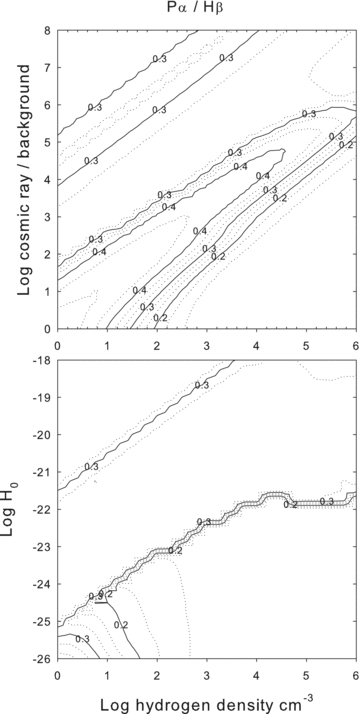
The H iPαλ1.87 μm to Hβλ4861 emissivity ratio is shown as a function of cloud parameters. These lines have a common upper n= 4 configuration; so changes in the relative intensities are due to changes in the nl populations within the n= 4 configuration. The Case B value is 0.34.
When the density is too low to collisionally mix the nl terms their populations tend to peak at smaller l since recombinations from the continuum and suprathermal excitation from ground tend to populate low-l levels. It is only when the density becomes large enough for l-changing collisions to mix the l levels that the well l-mixed limit is reached. This makes the Pαλ1.87 μm/Hβλ4861Å intensity ratio depend on density.
Fig. 7 shows that the Pα/Hβ intensity ratio does not vary over a broad range. The extra-heating case, shown in the lower panel, has a Pα/Hβ ratio in the range of 0.2–0.3, below the Case B ratio of 0.34 at 104 K and low densities. The cosmic ray case has a Pα/Hβ intensity ratio that varies between ∼0.2–0.4, within a factor of 2 of the Case B ratio. The range is larger because suprathermal electrons excite the atom for nearly all temperatures. These non-thermal excitations are mainly to np terms and create a distribution of nl populations that differs from the recombination case. This line ratio remains a good reddening indicator because of the relatively modest range in the predicted values when combined with the very wide wavelength separation of the two lines.
3.4 Chemical and ionization state of the gas
The two non-radiative heating cases, while having similar overall trends, have very different detailed properties, which we examine next. Fig. 8 shows predictions for a vertical line in Figs 1–3 corresponding to nH= 103 cm−3 and varying non-radiative heating rates. The independent axis gives the extra-heating rate pre-coefficient and the cosmic ray density relative to the Galactic background. These parameters were chosen to cross the region where the physical conditions in Figs 1–3 change abruptly. The left-hand panels show the extra-heating case and the right-hand panels the cosmic ray case. The second from the bottom panels of Fig. 8 show the kinetic temperature. The discontinuous jump in temperature, the regions where the contouring in Figs 1–3 become ragged, is clear. The lowest panels show the molecular, atomic and ionized fractions of hydrogen. The upper right-hand panel of Fig. 8 shows some heating and excitation efficiencies for the cosmic ray case. In all cases the temperature and ionization of the gas increases to the right-hand side as non-radiative energy sources become more important.
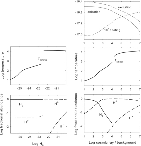
This shows the thermal and physical state along a vertical line at nH= 103 cm−3 in the previous contour plots. The left-hand panels are the extra-heating case while the right-hand panels are the cosmic ray case. The non-radiative rates are the independent axis in each panel. The range in both was adjusted so that the phase transition, where many physical quantities change abruptly, occurs near the middle of the independent axis. The ionization and temperature increase to the right-hand side as the non-radiative heating rates increase. The top right-hand panel shows the cosmic ray heating, ionization and line-excitation efficiencies. Cosmic rays ionize and excite predominantly neutral gas and heat ionized gas. The abrupt change in temperature, shown in the second to bottom pair of panels, is more extreme in the extra-heating case. The two lower panels show the physical state of hydrogen. There is a mix of atomic and molecular gas in the cosmic ray case due to the ionization and dissociation that they produce in cold neutral gas.
Both non-radiative heating cases have discontinuous jumps in temperature. These are due to inflection points in the gas cooling function that occur when more than one solution is possible. These stability issues are discussed further below. We first focus on the changes in the ionization of the gas shown in the lower two panels.
Table 3 compares physical conditions at three temperatures. The low and high temperatures of 100 and 104 K are near the extremes of the regions which produce the molecular and low-ionization emission. The mid-temperature was evaluated as close to 103 K as possible. This is a typical temperature for H2-emitting gas, as shown in Paper I. No stable thermal phase exists at exactly this temperature so the conditions at 700 K, the warmest stable region below 103 K, is given.
Physical conditions for the two cases at a range of kinetic temperatures.
| Species | T= 102 K | T∼ 700 K | T= 104 K |
| ne(Heat, cm−3) | 0.013 | 0.0089 | 0.59 |
| ne(CR, cm−3) | 0.92 | 9.3 | 155 |
| n(H2)(Heat, cm−3) | 952 | 940 | – |
| n(H2)(CR, cm−3) | 232 | 16 | – |
| n(H0)(Heat, cm−3) | 48 | 60 | 999 |
| n(H0)(CR, cm−3) | 768 | 975 | 863 |
| n(H+)(Heat, cm−3) | – | – | 0.0004 |
| n(H+)(CR, cm−3) | 0.80 | 8.4 | 137 |
In the extra-heating case thermal collisions are the only ionization source. The result is that at low temperatures the gas is predominantly molecular with a trace of H0. As the heating rate and temperature increase there is an abrupt change in the chemical state when the kinetic temperature approaches the dissociation potential of H2. The dissociation of H2 causes the particle density to increase and the mean molecular weight to decrease. Both cause the collisional rates, excitations, cooling and ionization, to increase. The result is a positive feedback process that causes an abrupt phase transition from H2 to H0. This is the reason that contours overlap in the lower panel of Figs 1–3.
This behaviour is in sharp contrast with the cosmic ray case. The effects of relativistic particles on a predominantly thermal gas has been well documented in a number of papers starting with Spitzer & Tomasko (1968) and most recently by Xu & McCray (1991) and Dalgarno et al. (1999). As shown in the upper right-hand panel of Fig. 8, cosmic rays excite, heat and ionize the gas. The curves marked ‘ionization’ and ‘excitation’ show the ionization and excitation rate (s−1) but have been divided by the cosmic ray-to-background ratio to remove the effects of increasing cosmic ray densities. The curve marked ‘heating’ has been similarly scaled and further multiplied by 107 to facilitate plotting. The fraction of the cosmic ray energy that goes into each process depends mainly on the electron fraction, ne/nH, the ratio of the thermal electron to total hydrogen densities. This electron fraction increases as the cosmic ray rate increases.
For low electron fractions a cosmic ray produces a first generation secondary electron that is more likely to strike atoms or molecules causing secondary excitations or ionizations. Radiation produced by line excitation or recombination following ionization will be absorbed by dust which then reradiates the energy in the far-IR (FIR). Relatively little of the cosmic ray energy goes into directly heating the gas. As the electron fraction increases, moving to the right-hand side in Fig. 8, more of the cosmic ray energy goes into heating rather than exciting or ionizing the gas. This is because for larger electron fractions the secondary electrons have a greater probability of undergoing an elastic collision with a thermal electron. This adds to the thermal energy of the free electrons and so heats the gas.
The effect is to produce a more gentle change in the ionization of the gas as the cosmic ray rate is increased. Ionization and dissociation are mainly caused by non-thermal secondary particles. Significant levels of dissociation or ionization exist at temperatures that are too low to produce these effects by thermal collisions. The lower two panels of Fig. 8 show how the H2 and H0 fractions change. In the cosmic ray case they change continuously until the thermal instability point is reached. Although a jump still occurs, the change in temperature is mitigated by the more continuous change in ionization and molecular fractions. This is to be contrasted with the extra-heating case where the gas is almost entirely molecular or atomic with little mixing of the two phases.
Some specific values are given in Table 3. At the lowest temperature, 100 K, nearly all H is molecular in the extra-heating case, while in the cosmic ray case substantial amounts of H0 are present. There are even significant amounts of H+ at this temperature because of the ionization produced by the cosmic ray secondaries. At the highest temperature shown, 104 K, nearly all H is atomic in the extra-heating case while a substantial amount of H+ is present in the cosmic ray case.
A substantial population of H0 and H+ is mixed with H2 in the cosmic ray heated gas. Molecular regions become far warmer and have far fewer H+ ions mixed with H2 in the extra-heating case. This leads to the most important distinctions between the two cases. Ions have larger collision cross-sections so are more active in altering the level populations of H2, as shown in Table 2. The H2 populations will be different as a result. Further, H0 and H+ can undergo ortho–para exchange collisions with H2. This process will be far more rapid in the cosmic ray case and will be another distinction between the two cases.
3.5 Thermal state of the gas
Fig. 8 shows that both cases have temperatures that change discontinuously. The origin of these jumps is described here. We concentrate on the extra-heating case where the effects are the largest.
Fig. 9 shows gas coolants as the extra-heating rate is varied across Fig. 8. The coolants leftward of the discontinuous break are classical atomic and molecular ‘PDR’ coolants. A Galactic PDR is the H0 region adjacent to galactic regions of star formation (Tielens 2005). These lines can be detected by current and planned IR instrumentation.
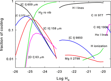
This identifies the most important cooling transitions for the extra-heating case shown in Fig. 8. The cooling shifts from the IR when the gas is cold and molecular, regions with log H0 < − 23, into the optical and UV when the gas is warm and ionized.
The gas abruptly changes from H0 to H+ at the discontinuity where the temperature jumps from ‘warm’(∼103 K) to ‘hot’(∼104 K). The coolants on the hot side are mainly emission lines of atoms and ions of the more common elements. The strongest coolant, marked ‘H i lines’, is the set of Lyman lines that are collisionally excited from the ground state. Although their intrinsic intensity is large they do not escape the cloud because of the large H i line optical depths and the presence of dust. These lines are absorbed by dust as the photons undergo multiple scattering. This is an example of a process that cools the gas by initially converting free electron kinetic energy into line emission which is then absorbed by, and heats, the dust. The energy eventually escapes as reprocessed FIR emission. Note that the gas and dust temperatures are not well coupled for the low densities found in these filaments. The dust is generally considerably cooler than the gas.
The behaviour shown in the two previous figures, with discontinuous jumps in the physical conditions, is due to well-known thermal instabilities in interstellar clouds. Fig. 10 shows the calculated cooling rate for a unit density and, again, the extra-heating case. The heating rate is varied and the temperature determined by balancing heating and cooling. We plot the cooling as a function of temperature rather than the heating rate to make it easier to compare these results with previous calculations.
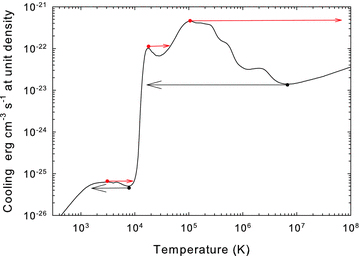
The cooling function for gas with unit density and a range of extra-heating rates. The heating is varied and the equilibrium temperature determined. The derived gas kinetic temperature is used as the independent variable to better compare with previous calculations and so that thermal stability can be judged. The arrows indicate regions where the gas will undergo a discontinuous jump in temperature to avoid thermally instable regions. A gas that was originally cold and molecular would follow the curve moving from left- to right-hand side while initially hot gas would move from right- to left-hand side.
The overall shape of the cooling function is discussed, for instance, in the review by Dalgarno & McCray (1972). At low temperatures cooling is mainly by molecules and low-lying levels within ground terms of atoms and first ions of the abundant elements. At low temperatures cooling usually involves changes in levels which have excitation energies of ≤103 K. The cooling increases as the Boltzmann factor for excitation increases and reaches a peak at ∼103 K where the Boltzmann factor reaches unity. The cooling then declines as T increases further due to the T−1/2 dependence of the Coulomb focusing factor. Starting at roughly 5000 K lines involving changes in term become energetically accessible, increasing the cooling, and producing a peak at ∼104 K. The decline after the peak is again due to the T−1/2 dependence of the collision rate coefficient when the Boltzmann factor has reached unity. The similar peak at ∼105 K is due to transitions involving changes in electronic configuration in ions of second and third-row elements.
The form of the cooling curve is affected by the presence of dust. Many of the most important coolants in a dust-free mixture, such as iron, calcium, silicon and others, are strongly depleted when dust forms. The result is that cooling is less efficient due to the loss of these gas-phase coolants. This is the major reason that the cooling curve differs from the solar abundance case.
Thermal instabilities cause the gas to have a memory of its history. The present state of the gas will depend on whether it approaches thermal equilibrium from the high or low-temperature state. One possibility is that the filaments cooled down from the surrounding hot-ionized plasma (Revaz, Combes & Salomé 2008). They would have reached their current state after moving from right- to left-hand side in Fig. 10. In this case the gas would follow the leftward-pointing arrows when it passed the unstable regions. Filaments originating as cold molecular gas, perhaps in the ISM of the central galaxy, would move from left- to right-hand side and would follow the rightward-pointing arrows. Different regions of the cooling curve are reached by a heating or cooling gas. This difference could provide a signature of the history of the gas.
3.6 The grain/molecule inventory and the history of the gas
The dust content and molecular inventory provides a constraint on the history of the filaments. If the filaments formed from the surrounding hot X-ray plasma they would likely be dust-free. Properties of dust-free clouds within a galaxy cluster were examined by Ferland, Fabian & Johnstone (1994) and Ferland, Fabian & Johnstone (2002). If the gas originated in the ISM of the central galaxy it would most likely contain dust, as we have assumed so far.
The dust-free H2 formation time-scales are ∼2.5 dex longer than those in a dusty environment. Unfortunately the ages of the filaments are poorly constrained. Hatch et al. (2006) find that a filament in the Perseus cluster with a projected length of ∼25 kpc and a velocity spread of ∼400 km s−1. The corresponding expansion age is ≥7 × 10⁷ yr. This is comfortably longer than the formation time for a dusty gas. H2 could only form in the dust-free case if the density is considerably higher than expected from typical pressures. This is possible but unlikely. We return to this question below.
The stable thermal solutions presented in the remainder of this paper are limited to those on the rising-temperature branch of the cooling curve. This, together with our assumed dust content, implicitly assumes that the gas was originally cold and dusty. In practice this means that the temperature solver determines the initial temperature with a search that starts at low temperatures and increases T to reach thermal equilibrium.
4 PROPERTIES OF CONSTANT-PRESSURE CLOUDS
4.1 Equation of state
The equation of state, the relationship between gas density and the temperature or pressure, is completely unknown for the filaments. Possible contributors to the total pressure include gas, turbulent, magnetic, cosmic ray and radiation pressures. The gross structure of the filaments, forming large lines or arcs, is reminiscent of magnetic phenomena like coronal loops. This suggests that magnetic fields guide the gas morphology with the field lines lying along the arc. Gas would then be free to flow along field lines, the long axis of the filaments, but not across them.
We assume that the gas pressure within the filaments is the same as the gas pressure in the surrounding hot gas, nT= 106.5 cm−3 K, found by Sanders & Fabian (2007) in the Perseus cluster. The magnetic field must then be strong enough to guide the cool material and so maintain the linear geometry despite any motion with respect to the surrounding hot gas. A magnetic field of ∼100 μG has an energy density equivalent to a thermal gas with nT= 106.5 cm−3 K so a field stronger than this is needed. Little is known about the filament geometry at the subarcsec (δr≤ 35 pc at Perseus) level and nothing is known about the magnetic field strength within the filaments. Magnetic confinement does provide a plausible explanation for the observed geometry however.
Fig. 11 shows the gas pressure in conventional ISM unit (P/k=nT cm−3 K) for the two cases. If individual subcomponents that make up the filaments have constant pressure then they will lie along one of these contour lines.
The log of the gas pressure, expressed as P/k=nT (K cm−3), is shown as a function of the hydrogen density and (top panel) the cosmic ray rate relative to the Galactic background and (bottom panel) the extra-heating rate. For comparison inner regions of the Perseus cluster have nT≈ 106.5 cm−3 K.
The dynamic range in Fig. 11 is large. The solid line in Fig. 12 corresponds to our preferred pressure of nT= 106.5 cm−3 K. The dashed lines in the figure show pressures 0.5 dex to either side of this value. As we show next, regions where the contours exceed a 45° angle, and where the ± 0.5 dex contours nearly overlap, are thermally unstable.
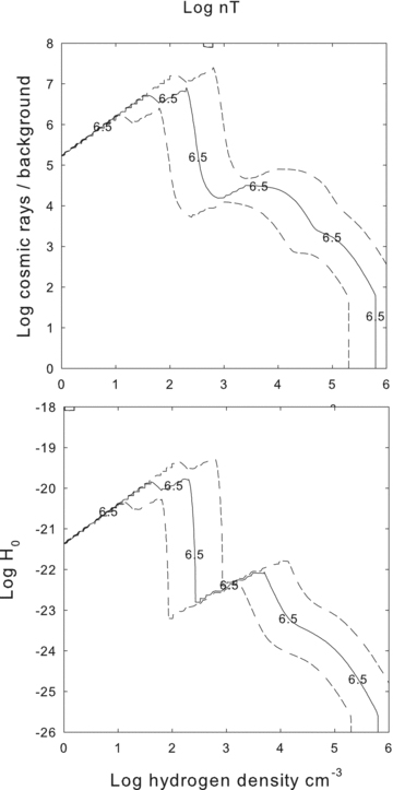
The solid contour corresponds to the preferred gas pressure P/k=nT= 106.5 cm−3 K. The dotted lines correspond to gas pressures 0.5 dex above and below this value. Regions where the contours have a steeper than 45° slope, where the contours nearly overlap, are thermally unstable.
4.2 Thermal stability
The upper panel of Fig. 13 shows the gas cooling rate along the isobaric log nT = 6.5 contour in Fig. 12. Both heating cases are drawn in each panel. The figure shows the cooling as a function of temperature rather than the heating rate so that the gas stability can be more easily judged. The detailed cooling properties of the two sources of non-radiative heating are quite different, as can be seen from the physical properties shown in Fig. 8 and listed in Table 3. The line marked ‘temperature−1’ shows the approximate form of the second term in equation (13). Regions where the slope of the cooling function is steeper than this are unstable. The lower panel of Fig. 13 shows the product of the cooling and the temperature. Expressed this way, regions with negative slope are unstable. Two distinct phases, corresponding to cold molecular and warm atomic/ionized, exist.
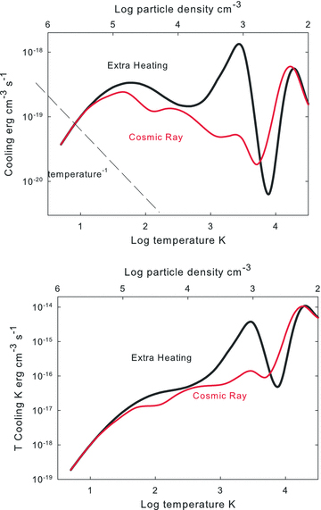
The solid lines in the upper panel give the volume cooling rates for the two cases as a function of the temperature (the lower independent axis) and particle density (the upper axis) along the P/k=nT= 106.5 cm−3 K isobaric contour of the previous figure. Regions where the slope of the cooling curve is steeper than the dashed line marked temperature−1 in the upper panel are thermally unstable. The lower panel shows the product of the cooling and the temperature. Regions where this product has a negative slope are unstable.
The upper axis in Fig. 13, and the figures that follow, gives the particle density along the isobaric line while the lower axis gives the kinetic temperature. Temperature and density are related since the product nT is constant. Note that the density n is the total particle density not the hydrogen density. For molecular regions the total particle density is about half the hydrogen density while in ionized regions it is about twice due to the presence of free electrons.
Fig. 14 shows the cooling time for the cases shown in Fig. 13 The cooling time will determine how quickly the gas can respond to changes in the environment. It also determines how quickly thermally unstable gas will heat or cool and reach stable regions of the cooling curve. These times are short compared with time-scales over which the galaxy cluster changes and are far shorter than the H2 formation time-scales mentioned above.
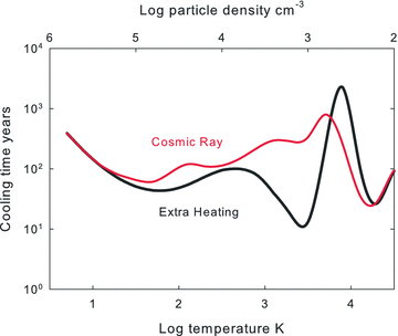
The cooling time-scales for the two cases shown in the previous figure is shown. Gas in unstable regions of the previous figure will move to a stable portion of the cooling curve on this time-scale.
4.3 Spectrum emitted by a homogeneous cloud
The full emitted spectrum is computed for each point along the isobaric line in Fig. 12. Emissivities 4πj of a few representative lines are shown in Fig. 15. The luminosity of a line will be the integral of 4πj over the volume of the emitting region.
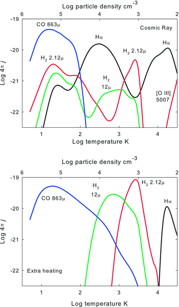
The emissivities, the emission per unit volume, are shown for several emission lines along the isobaric line corresponding to P/k=nT= 106.5 cm−3 K. The total particle density and temperature are indicated as the independent axes. The upper panel is the cosmic ray case and the lower panel is for extra-heating.
Most of the lines shown in Fig. 15 will be optically thin for any reasonable column density. In this case their emissivity has no explicit dependence on column density. If we can neglect internal reddening, a good approximation for the IR and radio lines but an additional uncertainty for optical or UV transitions, then the line luminosity is the integral of the emissivity over the volume containing gas. This is simple since the luminosity of an optically thin line is simply proportional to the total volume of emitting gas rather than on details of how the gas is arranged.
The CO lines are more problematic since lower J transitions are generally optically thick in the Galactic ISM. The emissivity of the CO J= 3 → 2 λ863 μm transition is shown rather than the lower J lines normally observed (Salomé et al. 2006), since it is more likely to be optically thin, if the column density of CO is large enough to thermalize an optically thick line then the luminosity will be set by the gas kinetic temperature and the cloud area rather than on the emissivity. It is by no means certain that the λ863 μm will be optically thin in the filaments and we shall return to the CO line spectrum below.
Fig. 15 shows that different lines form at different temperatures and densities because, as Fig. 8 shows, atoms and molecules exist at different regions with little overlap.
Paper I showed that H2 lines in the filaments are much stronger relative to H i recombination lines than is found in normal star-forming regions like Orion. H i recombination lines will have a peak emissivity that is weighted towards the coolest and densest regions where H+ is present, as shown in equation (9) and Fig. 5. This is indeed the case in the extra-heating case as shown in the lower panel of Fig. 15, where we also see that the H i and H2 lines form in gas with distinctly different densities and temperatures.
The extra-heating case, shown in the lower panel of Fig. 15, is simplest and we consider it first. Lines excited by thermal collisions tend to form in warmer gas because of the exponential Boltzmann factor. Low-excitation H2 lines such as λ12.28 μm form in cooler gas than the H2λ2.12 μm, which has an upper level with an excitation potential of ∼7000 K, in the extra-heating case.
The emissivities of the Hα and H2 lines have two local peaks in the cosmic ray case, as shown in the upper panel of Fig. 15. The lower temperature peak is due to the direct excitation of H i and H2 lines by secondary electrons. Excitation to H2 electronic levels that then decay into excited states of the H2 ground state, a process analogous to the photon Solomon process (Shaw et al. 2005), contributes to the H2 emission. The higher temperature peak occurs when cosmic rays heat the gas to a warm enough temperature to excite H2 transitions with thermal collisions. Eventually, in the highest T regions of the figure, the gas becomes warm enough to be predominantly ionized and the H i lines begin to form by recombination.
The hydrogen emission-line spectrum is predicted to be different from Case B relative intensities in regions where the lines form by collisional excitation of H0 rather than by recombination of H+. Fig. 16 shows the predicted intensities of the brighter optical and IR lines relative to Hα. There are two reasons for differences from simple Case B, the first being the large range in kinetic temperature along the isobaric line. The standard Case B spectrum is most often quoted for T= 104 K, appropriate for a photoionized cloud. The fact that collisional processes excite the lines in this environment cause further deviations from Case B.
The intensities of several strong optical and IR H i lines are shown for points along the isobaric line corresponding to log nT= 6.5. The total particle density and temperature are indicated as the independent axes.
Table 4 compares the H i spectrum for two points along the constant-nT line with Case B predictions. Little H i emission occurs for the extra-heating case at T≈ 300 K so only the cosmic ray case is given. The extra-heating and cosmic ray predictions agree at T≈ 2 × 10⁴ K because the gas is warm enough to collisionally excite the H i lines. The emissivity 4πj is ∼1 dex brighter than a pure-recombination H i spectrum because of the contribution of collisional excitation of H0. Note that the quantities given in Table 4 are the emissivity 4πj and not the emission coefficient 4πj/nenp given in, for instance, Osterbrock & Ferland (2006) The relative intensities of the H i lines are also different in the two cases. The H i lines at T≈ 300 K are mainly excited by non-thermal secondary electrons with collision rates that are proportional to the oscillator strength of the Lyman line. The emission at T≈ 2 × 10⁴ K is mainly produced by collisions with thermal electrons whose rates are dominated by the near-threshold cross-section. Case B applies when the lines form by recombination, which is not the case here.
Predicted H i emission spectrum.
| CR | CR,H | Ca B | Heat integrated | CR integrated | |
| log nH | 4 | 2.2 | 2 | integrated | integrated |
| log T | 2.5 | 4.3 | 4.3 | ||
| 4πj(Hα) | −19.85 | −19.96 | −21.01 | −20.029 | −20.171 |
| H i 3798 Å | 0.0132 | 0.000 76 | 0.0197 | 6.41(−3) | 0.0109 |
| H i 3835 Å | 0.0181 | 0.0112 | 0.0272 | 9.38(−3) | 0.0152 |
| H i 3889 Å | 0.0261 | 0.0172 | 0.0391 | 0.0145 | 0.0224 |
| H i 3970 Å | 0.0400 | 0.0286 | 0.0591 | 0.0244 | 0.0352 |
| H i 4102 Å | 0.0665 | 0.0531 | 0.0962 | 0.0459 | 0.0608 |
| H i 4340 Å | 0.125 | 0.116 | 0.173 | 0.102 | 0.120 |
| H i 4861 Å | 0.288 | 0.254 | 0.364 | 0.227 | 0.271 |
| H i 6563 Å | 1.000 | 1.000 | 1.000 | 1.000 | 1.000 |
| H i 1.875 μm | 0.121 | 0.0815 | 0.104 | 0.0839 | 0.0992 |
| H i 2.166 μm | 0.0082 | 0.0053 | 0.085 | 4.84(−3) | 6.35(−3) |
Table 4 shows that, although the H i lines have a far greater emissivity than is given by Case B, the relative intensities are not too dissimilar. This is because the relative intensities of the H i spectrum are most strongly affected by the transition probabilities that determine how a highly excited electron decays to ground rather than detail detains of how the electron became excited.
4.4 Allowed range of cloud density and temperature
The observed spectrum has a wide range of molecular and atomic emission, requiring that cloudlets with a range of densities and temperatures occur. Only some of the solutions shown in Fig. 15 will exist in a constant-pressure filament. The lowest temperature is set by the CMB temperature, the lowest temperature that molecules and grains will have. This low-temperature limit sets a high-density limit since the product nT= 106.5 K cm−3 is constant. Gas denser than nCMB∼ 106 K will remain at the CMB temperature, be overpressurized relative to its environment, and would expand. We do not consider gas denser than nCMB.
Thermal stability (Section 4.2 and Fig. 13) sets a low-density, high-temperature limit if the system is time steady. Gas on unstable parts of the cooling curve will move to regions of thermal stability on the cooling time-scale of the region. We only consider thermally stable solutions here and come back to discuss this point below.
Fig. 17 shows the emissivities of some strong lines that are produced near the low-density, high-temperature end of the cloud distribution. We concentrate on the optical spectrum in this figure since these lines form in warm gas and because their relative intensities can be measured with greater precision owing to the fact that this spectral range can be observed with a single entrance slit. The grey band in the upper right-hand side of each panel indicates regions which are thermally unstable. Most of the lines shown in the figure have peak emissivities that occur in stable regions. The predicted intensities of these lines will not depend greatly on the precise high-T cut-off of the cloud distribution.
![The emissivities of several of the prominent optical atomic and low-ionization lines seen in the filaments are shown. The lines include [O i]λ6300, [O ii]λ3727, [N i]λ5199 and [N ii]λ6584. The shaded rectangle indicates thermally unstable regions.](https://oup.silverchair-cdn.com/oup/backfile/Content_public/Journal/mnras/392/4/10.1111/j.1365-2966.2008.14153.x/2/m_mnras0392-1475-f17.jpeg?Expires=1750332713&Signature=cd85cdB1K5-vA3Vr1E8yJ~4ei-YMM5WqIIEJz-d8CBuwTMWnWrgof2pDnaikte~8F1-gWzE1zj1SxCW4rJnWLnSYKn0VcZ2qY3MGC1uvrpIos90PzVzLJS-FdMTYnox74nV5D0D6uR4~viGo0v2f9TeVAt~1VSsIsLx1ZZ9TtfSRM6PKOmdApxsI2stfVMAUdyxQwpblHUvSzMwCkRHxzR8pVsVi~HGLP35weAoLXO80m0DjF4ylvShHEuLNDlOZeIq2GTsu5zP7YtcP6ff7e2mIypU0lCiOTFbcVEYs65maWzG7zgSNRW3DKLqu4mtG42Q-XHRUYQwJTJ6PH5GXjQ__&Key-Pair-Id=APKAIE5G5CRDK6RD3PGA)
The emissivities of several of the prominent optical atomic and low-ionization lines seen in the filaments are shown. The lines include [O i]λ6300, [O ii]λ3727, [N i]λ5199 and [N ii]λ6584. The shaded rectangle indicates thermally unstable regions.
Fig. 18 shows some fainter lines which are currently unobserved in the Horseshoe filament in the Perseus cluster which we model in detail below. Some, for instance, [O iii]λ5007 Å, will be very sensitive to the thermal stability cut-off since the peak emission occurs in unstable regions. We show below that these lines can discriminate between the two non-radiative heating processes.
![The emissivities of several optical atomic and low-ionization lines that are either sensitive to the thermal stability cut-off or which might discriminate between the two non-radiative heating models we discuss. The lines include [O iii]λ5007, [Ne iii]λ3869 and He iλ5876. Hα is shown for reference. The shaded rectangle indicates thermally unstable regions.](https://oup.silverchair-cdn.com/oup/backfile/Content_public/Journal/mnras/392/4/10.1111/j.1365-2966.2008.14153.x/2/m_mnras0392-1475-f18.jpeg?Expires=1750332713&Signature=wRjqSys8ZEWSqi24MHcn38edaEGP7-uQY8VVScloaCPuJFIg4mPKA~t-wyr0Ko~1cqqmxTWidSw53IUEkl~j93XARjabumqWrN7~w07WTlYkUlByEQqQdwF0ioCkMxE6KkeJNZaSKK8s1TKwZUu~WWvh7swqI5X9K28YObUVzMtMdYaeyp2r5KpGYIOnh6uy9RhSmXceQJ~q6Cz21OLiVdtvt9grYuQ4CX4rb9iMt0IGJhZySmVRNPL8v9kNoha8UXssCOrhDiQD5SZrAnjWdPiq9RdlOvyE5vTJ2hi-Bvg9GVylgvJvWObKC1Pc6bDQTybggT1fYavRw3~kbGE2JQ__&Key-Pair-Id=APKAIE5G5CRDK6RD3PGA)
The emissivities of several optical atomic and low-ionization lines that are either sensitive to the thermal stability cut-off or which might discriminate between the two non-radiative heating models we discuss. The lines include [O iii]λ5007, [Ne iii]λ3869 and He iλ5876. Hα is shown for reference. The shaded rectangle indicates thermally unstable regions.
5 EMISSION FROM A DISTRIBUTION OF CLOUDS
5.1 The need for clouds with a range of properties
The spectrum shows that emission from both molecular and ionized gas comes from gas that is nearly spatially coincident (Salomé et al. 2008b). Physically this requires that gas with a variety of densities contributes to the net emission detected by the entrance aperture of a spectrometer.
No one choice of cloud parameters can reproduce the full range of molecular, atom and ionic emission. Figs 4 and 5 show that H i and H2 emission originate in warm and hot regions, respectively. The observed [N ii] or [O ii] emission cannot originate in the H2 region. Gas with a range of temperature and ionization must contribute to the observed emission.
The Galactic ISM has two or more thermally distinct phases that are in pressure equilibrium (Field, Goldsmith & Habing 1969). Fig. 12 shows that gas with two temperatures but the same pressure exist for some values of the non-radiative heating rates. This occurs for cosmic ray fluxes ≈4.2 dex times the Galactic background and for heating rate pre-coefficients of log H0≈−22.5. The range in gas properties for these two points is not broad enough to produce the observed range of emission however. For instance, in the cosmic ray case the two hydrogen densities are ≈103 and ≈104.3 cm−3, corresponding to kinetic temperatures of T≈ 103.5 and ≈102.2 K. Gas with this pair of densities, when co-added in the appropriate mix of filling factors, can account for some of the H i and H2 emission but none of the optical forbidden lines, as shown in Fig. 17.
The full range of thermally stable clouds shown in Fig. 13 must exist and contribute to the spectrum. It is then necessary to adopt a weighting function, as described next, to decide how to co-add clouds with different conditions. This weighting function is not a physical model for why this mix of clouds exists. Rather it represents a parametric way of solving the spectroscopic problem by specifying how the volume of clouds depends on density. We will end up with an empirical fit to the spectrum and finally discuss various scenarios that might establish this range of conditions.
5.2 Formalism
The physical picture is that the aperture of the spectrometer takes in emitting material with a range of densities and corresponding temperatures but a single pressure. This might occur, for instance, if the non-radiative heating rate is not uniform in space or time. Gas would heat up or cool down, on the cooling time-scale given in Fig. 14, in response to changes in the heating. The density and temperature would change to maintain constant pressure but clouds with a variety of densities and temperature would contribute to the emission from a region on the sky.
 (erg cm−3 s−1) integrated over a distribution of clouds is given by
 ), is similarly defined as

 and the total volume containing gas v (cm3) by


The physical meaning of these quantities is as follows. The volume v is the total volume containing gas. The gas within this volume has a range of density and temperature and may be molecular, atomic or ionized. The line emissivity  takes into account both the atomic physics of the emission process and the fact that a line is only emitted for certain combinations of density and temperature. The weighting parameter α determines the amounts of gas at various densities. The density
  depends on α since this sets how much weight is given to gas at various densities. It further depends on thermal stability criterion which sets nlow.
There are three free parameters, the lower and upper density bounds nlow and nhigh and the power-law index α. Physically motivated limits are used to set the density bounds in equation (17). As described in Section 4.4, thermally unstable densities are excluded from the integrals. This is equivalent to assuming that gas that lies on unstable portions of the cooling curve, shown in Fig. 13, will quickly move to stable regions so that the volume is fully filled by stable gas. The CMB temperature is assumed to set a lower limit to the kinetic temperature which then sets the upper limit to the density since the product nT is held fixed. This leaves only α as a free parameter.
5.3 Dependence on α
The full emission-line spectrum, with many hundreds of thousands of lines, is computed for each point along the isobaric curve illustrated by Fig. 15. The emissivity of each line is stored and integrated over density using equation (17). Integrated predictions are presented relative to Hα since it is easily observed and, of the bright optical lines, is the least affected by reddening.
Fig. 15 shows that different lines have emissivities that peak in different regions along the isobaric line. Lines that are formed in warm or hot ionized gas, such as the [S ii] or [O ii] optical lines, will form in nearly the same region as Hα itself as shown in Figs 17 and 18. We expect that the intensities of such lines relative to Hα will have little dependence on α but will depend on the chemical composition and the energy source. This is in contrast with molecular lines, such as the CO or H2 lines shown in Fig. 15, which form in gas that is much colder and denser that the gas producing the H i emission. Because of the form of the filling factor function we expect that molecular lines will be stronger relative to Hα for α close to 0 and that the intensity ratio decreases as α becomes more negative.
Fig. 19 shows the predicted line intensities as a function of α. Lines that form along with Hα, such as [S ii]λλ6716, are not strongly sensitive to the value of α. The line ratio is constant in the extra-heating case because Hα forms only in ionized gas along with the [S ii] lines. The ratio decreases for large values of α in the cosmic ray case because this gives the strongest weight to the molecular regions where the H i lines are formed by suprathermal excitation of H0. For the regions where the line ratio is a constant the intensities reflect the abundances of the elements and the underlying heating process rather than the integration process.
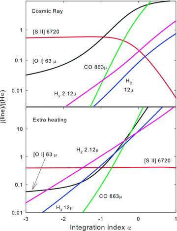
The integrated intensities of some strong lines are shown as a function of the power-law index α. The upper panel shows the H i Hα emissivity  . The middle and lower panels show the predicted intensities of other lines relative to Hα for the cosmic ray (middle panel) and extra-heating (lower panel) cases.
The intensities of molecular lines relative to Hα have a strong dependence on α. The power-law index α affects how the dense and cold molecular regions are added to the hotter ionized gas. Fig. 19 shows that such lines as [O i]λ63 μm, H2 2.12 μm and CO λ863 μm have powerful dependencies on α. We will use these lines to determine α in the following section.
Fig. 20 shows the Hα emissivity and mean density as a function of α. The upper panel shows the emissivity  of H i Hα as defined by equation (16). The emissivities are quite similar for when α is very small since this give greatest weight to the warm ionized regions where the emissivities are similar. They differ for large α since this weights the cold dense regions where suprathermal excitation of H i is important in the cosmic ray case. The total volume of gas in all forms, molecule, atomic and ionized, will be the observed luminosity of the Hα line divided by this emissivity, as given by equation (20). The lower panel of Fig. 20 shows the mean density defined by equation (18). The two cases differ slightly at low densities because the low-density cut-off given in equation (19) is set by the thermal stability requirement. The total mass of gas in the filaments can be derived from the Hα luminosity and the information given in this figure together with equation (21). Note that although we give these results for Hα there is enough information in the tables and figures to do this with any emission line.
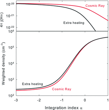
The upper panel shows the H i Hα emissivity  as a function of the power-law index α. The lower panel shows the integrated density defined by equation (18).
5.4 The observed spectrum
The next step is to use the observed intensities of molecular lines relative to Hα to set the power-law index α. This requires an observed spectrum that extends across the optical into the FIR. We take the Horseshoe region of the Perseus cluster as representative. It is relatively isolated, at a projected distance of 25 kpc from the centre of NGC 1275, so confusion with other sources is minimized. Its spectrum does not have underlying stellar absorption lines so optical H i lines can be measured without stellar contamination.
The upper section of Table 5 gives the line ratios observed in the Horseshoe region together with predictions from the two models. The optical (Gemini GMOS) and near-IR (NIR) (UKIRT CGS4) data are from Hatch et al. (2006) and Hatch et al. (2005), respectively, and the mid-IR data are from Johnstone et al. (2007). All of the observed quantities in Table 5 have been corrected for an assumed Galactic extinction of E(B−v) = 0.163 (Schlegel, Finkbeiner & Davis 1998).
Upper: Observed and predicted line strengths near the Horseshoe position 11 region of Conselice et al. (2001). Column 1 lists the emitting species, column 2 is the wavelength in microns, column 3 is the observed, extinction corrected flux ratio of each line with respect to Hα, column 4 is the line flux ratio with respect to Hα predicted by the extra-heating model, column 5 is the line flux ratio with respect to Hα predicted by the cosmic ray heating model. Note that the optical, NIR and MIR lines are each observed though a different aperture. See Fig. 21 for a visualization of each aperture. Lower: Observed Hα surface brightness, S(Hα) (erg s−1 cm−2 arcsec−2) and luminosity, L(Hα) (erg s−1) corresponding to the same region that the optical line ratios were extracted from. The integrated line emissivity averaged over the distribution of clouds,  , (erg s−1 cm−3) defined by equation (16), and the density averaged over the distribution of clouds,
  ), defined by equation (18) in the wave heated and cosmic ray heated models are also tabulated.
| Species | λ(μm) | F(line)/F(Hα) observed | Predicted/observed extra heat | Predicted/observed cosmic ray |
| α | −2.10 | −0.35 | ||
| H i | 0.4861 | 0.24 | 0.87 | 1.04 |
| [O iii] | 0.5007 | < 0.03 | ||
| [N i] | 0.5199 | 0.06 | 1.88 | 1.66 |
| He i | 0.5876 | 0.04 | 6.4 × 10⁻⁵ | 0.37 |
| [O i] | 0.6300 | 0.19 | 1.00 | 0.93 |
| H i | 0.6563 | 1.00 | 1.00 | 1.00 |
| [N ii] | 0.6584 | 0.71 | 0.29 | 0.34 |
| [S ii] | 0.6716 | 0.23 | 1.05 | 1.40 |
| [S ii] | 0.6731 | 0.17 | 1.15 | 1.08 |
| H2 | 1.957 | 0.09 | 1.28 | 0.81 |
| H2 | 2.033 | 0.03 | 1.44 | 1.41 |
| H2 | 2.121 | 0.08 | 1.54 | 1.02 |
| H2 | 2.223 | 0.02 | 1.38 | 0.77 |
| H2 | 12.28 | 0.03 | 1.00 | 1.00 |
| [Ne ii] | 12.81 | 0.06 | 4.6 × 10⁻³ | 0.46 |
| [Ne iii] | 15.55 | < 0.02 | ||
| H2 | 17.03 | 0.06 | 0.29 | 0.53 |
| S(Hα) | 1 × 10⁻¹⁴ | |||
| L(Hα) | 7 × 1039 | |||
 | 9.40 × 10⁻²¹ | 6.75 × 10⁻²¹ | ||
 | 300 | 2.63 × 10⁴ |
| Species | λ(μm) | F(line)/F(Hα) observed | Predicted/observed extra heat | Predicted/observed cosmic ray |
| α | −2.10 | −0.35 | ||
| H i | 0.4861 | 0.24 | 0.87 | 1.04 |
| [O iii] | 0.5007 | < 0.03 | ||
| [N i] | 0.5199 | 0.06 | 1.88 | 1.66 |
| He i | 0.5876 | 0.04 | 6.4 × 10⁻⁵ | 0.37 |
| [O i] | 0.6300 | 0.19 | 1.00 | 0.93 |
| H i | 0.6563 | 1.00 | 1.00 | 1.00 |
| [N ii] | 0.6584 | 0.71 | 0.29 | 0.34 |
| [S ii] | 0.6716 | 0.23 | 1.05 | 1.40 |
| [S ii] | 0.6731 | 0.17 | 1.15 | 1.08 |
| H2 | 1.957 | 0.09 | 1.28 | 0.81 |
| H2 | 2.033 | 0.03 | 1.44 | 1.41 |
| H2 | 2.121 | 0.08 | 1.54 | 1.02 |
| H2 | 2.223 | 0.02 | 1.38 | 0.77 |
| H2 | 12.28 | 0.03 | 1.00 | 1.00 |
| [Ne ii] | 12.81 | 0.06 | 4.6 × 10⁻³ | 0.46 |
| [Ne iii] | 15.55 | < 0.02 | ||
| H2 | 17.03 | 0.06 | 0.29 | 0.53 |
| S(Hα) | 1 × 10⁻¹⁴ | |||
| L(Hα) | 7 × 1039 | |||
| 9.40 × 10⁻²¹ | 6.75 × 10⁻²¹ | ||
| 300 | 2.63 × 10⁴ |
Upper: Observed and predicted line strengths near the Horseshoe position 11 region of Conselice et al. (2001). Column 1 lists the emitting species, column 2 is the wavelength in microns, column 3 is the observed, extinction corrected flux ratio of each line with respect to Hα, column 4 is the line flux ratio with respect to Hα predicted by the extra-heating model, column 5 is the line flux ratio with respect to Hα predicted by the cosmic ray heating model. Note that the optical, NIR and MIR lines are each observed though a different aperture. See Fig. 21 for a visualization of each aperture. Lower: Observed Hα surface brightness, S(Hα) (erg s−1 cm−2 arcsec−2) and luminosity, L(Hα) (erg s−1) corresponding to the same region that the optical line ratios were extracted from. The integrated line emissivity averaged over the distribution of clouds, , (erg s−1 cm−3) defined by equation (16), and the density averaged over the distribution of clouds, ), defined by equation (18) in the wave heated and cosmic ray heated models are also tabulated.
| Species | λ(μm) | F(line)/F(Hα) observed | Predicted/observed extra heat | Predicted/observed cosmic ray |
| α | −2.10 | −0.35 | ||
| H i | 0.4861 | 0.24 | 0.87 | 1.04 |
| [O iii] | 0.5007 | < 0.03 | ||
| [N i] | 0.5199 | 0.06 | 1.88 | 1.66 |
| He i | 0.5876 | 0.04 | 6.4 × 10⁻⁵ | 0.37 |
| [O i] | 0.6300 | 0.19 | 1.00 | 0.93 |
| H i | 0.6563 | 1.00 | 1.00 | 1.00 |
| [N ii] | 0.6584 | 0.71 | 0.29 | 0.34 |
| [S ii] | 0.6716 | 0.23 | 1.05 | 1.40 |
| [S ii] | 0.6731 | 0.17 | 1.15 | 1.08 |
| H2 | 1.957 | 0.09 | 1.28 | 0.81 |
| H2 | 2.033 | 0.03 | 1.44 | 1.41 |
| H2 | 2.121 | 0.08 | 1.54 | 1.02 |
| H2 | 2.223 | 0.02 | 1.38 | 0.77 |
| H2 | 12.28 | 0.03 | 1.00 | 1.00 |
| [Ne ii] | 12.81 | 0.06 | 4.6 × 10⁻³ | 0.46 |
| [Ne iii] | 15.55 | < 0.02 | ||
| H2 | 17.03 | 0.06 | 0.29 | 0.53 |
| S(Hα) | 1 × 10⁻¹⁴ | |||
| L(Hα) | 7 × 1039 | |||
| 9.40 × 10⁻²¹ | 6.75 × 10⁻²¹ | ||
| 300 | 2.63 × 10⁴ |
The lower section of Table 5 gives the observed Hα surface brightness, S(Hα), and luminosity L(Hα) corresponding to the same region that the optical line ratios were extracted from. The averaged line emissivity,  , and averaged density,
  , from the wave heated and cosmic ray heated models are also listed.
The observational data presented in Table 5 were measured from a variety of ground- and space-based telescopes. These facilities each have different entrance apertures, which we show overlaid on the Hα emission map of Conselice, Gallagher & Wyse (2001) in Fig. 21. As stressed by Johnstone et al. (2007), these aperture corrections make it difficult to combine observations taken with different instrumentation. The 2-μm NIR and optical spectra (Hatch et al. 2005, 2006) were combined by scaled them to the same observed Hα flux. The Hα flux in the NIR data was estimated from the observed Pα line flux assuming that the Pα/Hα intensity ratio has the Case B value (8.45) for T= 104 K. The MIR Spitzer observations of the low-J H2 lines were placed on the same flux scale as the optical/NIR lines by another method that did not assume Case B. Hα images of the region covered by the Spitzer entrance aperture were used to find the area covered by emitting gas and maps of the optical H i and MIR H2 emission were compared to introduce aperture corrections and derive flux ratios (Johnstone et al. 2007).
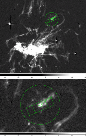
Entrance apertures of the various instruments used to determine the line ratios presented in Table 5 and in the text. Gemini GMOS: long thin rectangle, UKIRT CGS4: small rectangle centred on brightest knot. The two larger overlapping rectangles are the positions of the Spitzer IRS SH aperture. Line fluxes were averaged between these two nod positions. The large circle is the beam of the IRAM (CO 1–0) observations.
There are substantial uncertainties in the derived spectrum. The calculations presented above show that the Pα/Hα ratio is not expected to be given by Case B although the differences are not great (Table 4). The extinction within the filaments is unknown so no correction is made. Renormalizing the optical/NIR H i spectrum to agree with Case B intensities largely removes the effects of reddening. Given the uncertainties in both the observed and theoretical predictions our goal is to reproduce the spectrum to within a factor of 2.
Salomé et al. (2008b) detect the CO 1–0 line in the Horseshoe and note that the line is optically thick. This is in contrast to the optically thin optical and IR lines that are the focus of this paper. The observed flux of an optically thick line depends on the geometry while that of an optically thin line depends only on the volume of emitting gas.
Salomé et al. (2008b) derive a mass of 108 M⊙ for the region of the Horseshoe included in their 11 arcsec radius beam (see Fig. 21). We can derive the total mass from the luminosity of any emission line using equation (21). We measured the Hα luminosity in the IRAM beam from the data of (Conselice et al. 2001) as L(Hα) = 5.5 × 1040 erg s−1.
5.5 The predicted spectrum
We vary α to match the observed H2 12.28 μm/Hα intensity ratio of 0.03 (Table 5). This line ratio has several advantages. It has one of the widest ranges in excitation and ionization in the spectrum and so is a strong function of α. The IR H2 lines are, like the optical H i lines, optically thin so geometric effects do not enter. Finally, by comparing emission from an ion and molecule of the same element there are no additional uncertainties introduced by that fact that the composition is unknown. The uncertainty in the ratio is likely to be dominated by systematic errors which we cannot quantify.
This procedure gives α=−0.35 for the cosmic ray and α=−2.10 for the extra-heating cases. Both cases have negative α which, as equation (14) shows, means that the lowest density gas has the largest volume. We are led to a picture in which the molecular gas lies in cold and dense cores while the low-ionization emission originates in extended low-density regions. The ionized material may be located in extended envelopes surrounding the molecular cores.
The last two columns of Table 5 give the predicted line intensities relative to the observed values. A more complete set of predicted intensities is given in Appendix A. Our goal is to match the spectrum to within a factor of 2. Both heating cases do this for the majority of lines. The discriminants between the two cases are described in the next section.
The last two columns of Table 4 give the integrated H i spectra for the two cases. The predicted Pα/Hα ratio is 0.0839 and 0.0992 for the extra-heating and cosmic ray cases, not greatly different from the Case B ratio of 0.104. The Pα/Hβ is 0.37 for both heating cases and is 0.29 for Case B. These differences are significant but the wide wavelength separation of the line pairs make them useful reddening indicators.
5.6 The need for ionizing particles
Several emission lines indicate that the cosmic ray case best describes the heating and ionization of the gas. Most lines are matched by both cases to within our desired factor of 2. It is not possible to formally quantify a goodness of fit in Table 5 because the uncertainties are dominated by systematic errors which we cannot quantify. Rather we point to a few lines which clearly indicate that the cosmic ray case applies.
Figs 17 and 18 show the critical distinction between the two cases. The extra-heating case behaves as expected for a collisionally excited thermal gas. As the temperature increases, going from left- to right-hand side in the figures, we see lines of [O i], [N i], [N ii], [O ii], [O iii], He i and eventually [Ne iii], increasing in intensity. This corresponds to increasing ionization and excitation potentials as expected for a collisionally ionized gas. As stressed in the discussion of Fig. 8 the distribution of ions and molecules in the extra-heating case is sharply defined by temperature. At a given temperature hydrogen will be nearly all ionized, atomic or molecular with the change from one species to the next occurring over a relatively small range in temperature.
This behaviour is to be contrasted with the cosmic ray case. Here a certain level of ionization and excitation is present at all gas kinetic temperatures because the cosmic ray ionization rates are only indirectly related to temperature. The result is that some H0 is present in regions that are predominantly H2 or H+. We find the somewhat paradoxical result that the higher ionization (3.00 Ryd to create) [Ne iii]λ3869 Å line becomes strong at lower temperatures than the lower ionization (2.58 Ryd) [O iii]λλ5007, 4959Å lines. This is because of the importance of charge-transfer recombination in setting the ionization distribution of O. The process O+n+ H0→ O+n−1+ H+ is very fast for both O+ and O+2 but is slow for He+, Ne+ and Ne+2. Larger amounts of H0 are present in the cosmic ray case because of the mixing of different ionization species in the same region. The result is that the cosmic ray case produces significant [Ne ii]λ12.81 μm and [Ne iii]λ3869 Å emission without exceeding the upper limit to [O iii]λ5007 Å.
He iλ5876 Å provides another distinction between the cosmic ray and extra-heating cases. He0 is more efficiently ionized by suprathermal than by lower energy thermal particles due to its large ionization potential. The λ5876 Å line is in fair agreement with the observed value in the cosmic ray case while it is underpredicted by more than 4 dex in the extra-heating case.
Fig. 18 shows the fundamental tension experienced by the two cases. We do not include the thermally unstable temperatures indicated by the grey bar in the figure. The extra-heating case could only produce significant He i and [Ne iii] emission by including large amounts of unstable gas. This would overpredict the unobserved [O iii]λ5007 Å line by large factors. The cosmic ray case produces strong He and Ne emission while not overproducing [O iii].
Johnstone et al. (2007) discuss the puzzle posed by the observed [Ne iii] emission from filaments that do not show significant [O iii]λ5007 Å. Neon is special because of the high ionization potentials compared with other second row elements like N or O. [Ne iii] was not detected in the Horseshoe but was seen in another region where [O iii] was weak. Johnstone et al. (2007) suggested that a low kinetic temperature in the ionized gas, perhaps the result of enhanced abundances and cooling efficiency, might be the cause. Cosmic ray ionization is another possibility.
These calculations demonstrate that cosmic rays are needed to account for the spectrum. Suprathermal particles such as those produced by cosmic rays create a gas with a broad range of ionization at any one point. Charge-transfer recombination then produces the observed unusual ionization distribution of the heavy elements. Although we have explicitly considered cosmic rays, which are known to exist in the cluster environment, any source of ionizing particles would work as well. Although gentle heating by MHD waves is ruled out, MHD waves could still be the fundamental source of the ionization since high-energy particles may be produced in situ by MHD phenomena such as magnetic reconnection (Lazarian 2005).
Crawford & Fabian (1992) showed that photoionization by a very hard continuum source can produce the optical spectrum. High-energy photons produce primary and Auger electrons that have very high energies and so behave as ionizing particles. Their model worked for the same reasons that the cosmic ray model discussed above works. The ionizing particles generate a gas with a mix of molecules, atoms and ions, charge-transfer effects are important, and a peculiar low-ionization spectrum is produced. Photoionization by very hot objects is another viable source of the deduced population of suprathermal particles.
A form of mixing layers might also produce the ionizing particles. If hot ionized gas were to mix with cold molecular gas the resulting physical state would be determined by the microphysics of the collisional interactions rather than by the ratio of kinetic temperatures. Any energy source that deposits its energy as ionizing particles rather than as heat can produce the observed spectrum. Our predictions do not depend on the fundamental energy injection, only on the eventual production of a population of suprathermal particles. We shall refer to this as ionizing particle heating in the remainder of this paper to reflect the fact that there are many possible sources of these particles.
6 DISCUSSION
6.1 The geometry
Our deduced value of α=−0.35 corresponds to the majority of the volume being filled by low-density ionized gas. The density of the molecular regions is typically  times higher than the density of the ionized gas (Fig. 15). The ratio of volumes is then vmole/vion∼ 103α∼ 0.09. By contrast, most of the mass is in dense molecular cores. The mass depends on nα+1 so the ratio of masses is Mmole/Mion∼ 103(α+1)∼ 90. The small dense molecular cores may provide the reservoir of material for an extended halo of low-density ionized gas. If the gas is constrained to follow magnetic field lines then the individual clouds may resemble comets with a cold dense core and extended warm low-density tail.
The observed surface brightness in Hα and the predicted  , both listed in Table 5, can be combined with equation (22) to find the line-of-sight thickness of emitting material. The deduced thickness is d l= 1.0 × 1018 cm = 0.3 pc. Note that this is the thickness of the entire cloud, not just the H+ region, although most of this is filled by ionized gas.
This depth is similar to that found by Fabian et al. (2003) from fundamentally different assumptions. They assumed that the optical H i lines are formed by recombination with Case B intensities, that the pressure of the H i-emitting gas was equal to that of the surrounding hot gas, and that the gas was fully ionized with a temperature of ∼104 K. If the gas is excited by ionizing particles then H i is far more emissive than predicted by Case B due to the enhancement by collisional excitation (Table 4). This large enhancement makes up for the fact that hydrogen is not fully ionized across the volume so the H i emission measure, the product nenp dl, is much smaller. These two factors nearly cancel leading to a similar depth.
For this surface brightness argument to work the entire entrance aperture of the spectrometer must be covered by emitting gas. A slit width of 1 arcsec corresponds to a projected width of ∼350 pc at the distance of Perseus. Each cloud is ∼0.3 pc thick along the line of sight but must cover a region of the sky ∼350 pc across. The aspect ratio of the width to depth of the emitting gas is >103:1 since the region of the Horseshoe we observed is well resolved on the sky. This aspect ratio, although surprising, is similar to other geometric quantities in the system. Hubble Space Telescope observations show that the projected width of the narrowest parts of the filaments is ∼70 pc (Fabian et al. 2008) while they have lengths of tens of kpc. The filaments are composed of remarkably thin and long clouds.
The filaments are most likely composed of a network of much smaller threads. In the magnetic field dominated constant-pressure case assumed here gas is free to move along but not across field lines. The line surface brightness suggests that individual threads have a width of a fraction of a pc. We view this geometry from a direction that is nearly orthogonal to the field lines. This is an observational selection effect introduced by the way that isolated filaments were chosen for study. The narrowest filaments, with a width of 70 pc, must be composed of ∼102– 103 of these thin threads. If the threads are uniformly distributed across the filaments, and the filaments have a depth equal to their observed width, then the mean separation between threads is ∼10 pc, about 30 times their thickness.
There are two possible physical interpretations for our α power-law index. It could represent a radial gradient in density across a thread normal to the field lines. In this case the dense molecular regions would form a very small linear core with the lower density ionized gas surrounding it in a much larger cylinder. We consider this unlikely since gas could not move across field lines to change its density in response to changes in the heating. The more likely possibility is that the α index represents the variation of the density along magnetic field lines. In this picture the ionizing-particle density would vary with position or time, the temperature of the gas would adjust itself in response, and then expand or contract to maintain constant pressure. A magnetic field line would then have most of its volume occupied by lower density ionized gas intermixed with dense molecular regions. The cold dense molecular regions could become warm and ionized, and return to being cold and molecular, as the heating rate changes.
6.2 Internal extinction across a thread
The hydrogen column density through a thread normal to its surface is  . If the gas has a Galactic dust-to-gas ratio, as we have assumed, then the total visual extinction across a thread will be Av∼ 17 mag. The effects of this extinction depend on the geometry. The dense molecular regions, having most of the column density, would also be most extinguished. This region detected emits MIR and submillimetre emission where the extinction will have little effect. The column density through the partially ionized gas which produces most of the optical emission is small so this emission is not directly affected by internal extinction. We could not detect optical emission from ionized regions which happened to lie on the far side of the molecular cores of course.
6.3 The total mass at position 11
The total mass can be derived from the luminosity of any emission line using the formalism derived in Section 5.2. Section 5.4 derived an L(Hα) of 5.5 × 1040 erg s−1 for position 11 and the beam used by Salomé et al. (2008b). Equation (21) gives a total mass of 2.1 × 10⁸ M⊙. This is in reasonable agreement with the mass of 108 M⊙ derived by Salomé et al. (2008b) from observations of the CO 1–0 transition.
The mass of 2.1 × 10⁸ M⊙ derived from emission lines counts only the spectroscopically active gas. As Fig. 15 shows, little emission is produced by cold gas at the high-density end of the distribution. Gas denser than our high-density limit cannot exist and be in pressure equilibrium because the CMB sets the lowest possible temperature. However, there is no observational constraint that actually limits the amount of material that could be at this highest density and the CMB temperature. A large reservoir of very cold high-density gas could exist and remain undetected. Our derived mass is a lower limit as a result. Gas at the very coldest limit of the distribution could serve as the source of fresh material for the spectroscopically active regions.
6.4 The pressure of the molecular cores
A number of studies have estimated the pressure of the molecular gas. Next we compare these with our derived temperature and density which assume a pressure equal to that of the surrounding hot gas.
Jaffe et al. (2001) found a density nH > 105 cm−3 and T∼ 103.2 K from the distribution of H2 level populations. The gas pressure, nT > 108.2 K, was substantially higher than the pressure of the surrounding hot gas. For our best-fitting ionizing particle model most of the v= 0, low-J, H2 emission originates in gas with a temperature of about T∼ 101.3 K and a density nH∼ 105.2 cm−3, as shown in Fig. 15. Excited-v emission occurs at a higher temperature, T∼ 103.2 K, and lower density, nH∼ 103.3 cm−3. We do not present level-excitation diagrams in this paper but note that we have fitted the observed H2 spectrum, from which the H2 level-excitation populations were derived, to within a factor of 2. Our model produces a population distribution that is consistent with these observations.
Salomé et al. (2008a) argue that the filaments are composed of an ensemble of Galactic giant molecular cloud (GMC) like components. By analogy with GMCs they argue that the density in the CO region is several hundred particles per cubic centimetre and that the gas has a kinetic temperature of T≈ 20–40 K. The resulting pressure, nT≈ 103.3 cm−3 K, is 3.2 dex smaller than the pressure of the surrounding hot gas.
We avoid geometrical complexities by focusing on optically thin emission lines. Fig. 15 shows that the optically thin emissivity of the CO λ863 μm line peaks at Tk,CO≈ 20 K and n≈ 104.2 cm−3. This temperature is similar to the CO temperature quoted by Salomé et al. (2008a) but the density is considerably higher in keeping with our assumed high gas pressure. The difference is due to the higher cosmic ray density in our simulations. Well-shielded regions of Galactic GMCs are similarly heated by cosmic rays but with a considerably lower intensity equal to the Galactic background. The cosmic ray density that produced the peak in our simulations is ∼104 times the Galactic background. This accounts for the GMC-like temperatures at such a high pressure. It is not possible to make a specific prediction of the CO 1–0 brightness temperature without first deriving an explicit geometric model of the cloud, a task beyond the scope of this paper.
We conclude that both the H2 spectrum and CO brightness temperature are consistent with a gas pressure of nT= 106.5 K cm−3 and excitation by ionizing particles.
6.5 Gravitational stability
The stability of the material in the filaments to gravitational collapse may be influenced by a number of factors: basic geometry, turbulence and magnetic fields.
 and the density is 105n5 cm−3. For c5= 1, n5= 1 the thickness of the molecular material will be 0.3 pc, a similar scale to that inferred for the Hα emitting region. We infer above that the molecular material has a volume filling fraction about one tenth that of the ionized gas, so the size scale of the molecular material will be comparable to this. This suggests that the gravitational stability of the molecular component may have a significant role in determining the structure of the filaments.
Magnetic fields and turbulence may play a significant role in supporting the molecular material against gravitational collapse. The standard criterion for support against collapse by uniform magnetic fields is to compare the column density along a flux line to the critical value B/2πG1/2. If the dense material is threaded along flux tubes, this is not a significant constraint as it stands. Likely more important is the coupled effects of turbulence and randomly directed internal magnetic fields. These will act to increase the effective virial velocity of the material, and so support it against collapse.
However, both turbulence and random magnetic fields are inherently transient, and so must be driven in some fashion to maintain their role in supporting the material. In the local ISM, this driving is achieved by a number of processes, including star formation. While there is some evidence of star formation in the filaments, this appears to be a relatively localized phenomenon.
What will happen if part of the molecular material in a filament starts to undergo a gravitational collapse? We find that the cooling time-scale (∼102 yr) is significantly smaller than the dynamical time-scale (∼3 × 10⁵ yr), so the material may initially fragment. However, the enhanced density will mean that the net tidal force between the material and the surrounding diffuse envelope will increase, both allowing the filament to break up, and enhancing the net heating. This process may thus naturally maintain the filaments with marginal gravitational stability, in a similar fashion to that in which galactic discs are maintained with a Toomre Q parameter around unity. Note that if this is the case, it requires that the heating rate is determined by local processes, such as drag-driven reconnection.
6.6 The energy budget
The energy dissipation time-scale for the line-emitting material is short, requiring that the energy be replenished in situ. While it is clear from Fig. 15 that below 104 K the detailed cooling mechanisms depend on the temperature, from Fig. 13 the overall cooling rates do not depend strongly on these details. The heating need to power the emission regions in steady state ranges from λ∼ 10−19±1 erg cm−3 s−1 while the thermal time-scale of the gas is ∼102 yr (Fig. 14).


The time-scales for the cosmic ray heated case are somewhat longer. The Galactic background cosmic ray density corresponds to an energy density of ∼1.8 eV cm−3 (Webber 1998), mostly in high-energy nuclei. The cosmic ray intensity required to maintain the material at nT∼ 106.5 cm−3 K ranges between 102 and 106 times the Galactic background value, depending on the filament density (Fig. 12). Molecular regions are predicted to have a density of nH∼ 105 cm−3 and require a cosmic ray ∼103 times the background. The low-ionization gas requires a rate ∼106 times the background with a density of nH∼ 102.5 cm−3. For these values the energy dissipation time for the molecular and low-ionization regions are ∼103 and ∼5 × 10⁵ yr, respectively.
These replenishment time-scales are generally of the order of or longer than the cooling time (Fig. 14), the time required for the gas to adjust itself to a changing heating rate. This means that non-equilibrium effects, in which the ionization, heating and cooling decoupled from one another, may be important. The short heating/cooling times suggests that the gas pressure can fluctuate about its equilibrium value in response to variations in the environmental heating, and may drive sound waves. The resulting structures may be intrinsically quite dynamic and disequilibrium.


At high Reynolds number, the drag force is roughly equal to the ram pressure between the phases. At the relative density of the X-ray hot medium and the molecular gas, this would suggest that to prevent the dense material moving at free-fall velocities, the relative motion of the hot material must be at (nmol/nhot)1/2vff, which are not likely to be the case. The filament material may be transitory on a time-scale ∼vfil/g≃ 3 × 10⁶ yr, in which time the filament material will travel ∼1/2 (v/vKep)2 of the distance to the core of the cluster. Alternatively, their effective cross-section may be increased either by an effective viscosity or by magnetic fields.
The interphase drag will lead to magnetic field lines in the diffuse phases becoming wrapped around the dense material. This suggests that the magnetic structure may be somewhat like the bubble in the solar wind maintained by the earth's magnetosphere. The resulting magnetic segregation would limit high-energy particle transport into the molecular material. It is likely that some high-energy particles will be able to leak in, either through magnetic neutral points, as a result of turbulent motions, or by diffusion resulting from field inhomogeneities. Alternatively, the drag-driven turbulence may itself be the source of the high-energy particle flux, as a result of reconnection events.
Overall, it is clear that the dissipation of the energy resulting from buoyancy has potential as a source of heating for the filaments. However, if this is the source of the heating, the means by which the energy is transformed into the non-thermal ionizations which we infer are the immediate means by which the molecular material is heated must be complex.
6.7 What is the source of the ionizing particles?
The chemical-ionization state of the gas strongly suggests that the heating and ionization is produced by ionizing particles. Several considerations suggest that the population of ionizing particles is not produced by a strongly enhanced version of Galactic cosmic rays.
The energy density Galactic cosmic rays is dominated by particles with energies around 1 GeV in the solar neighbourhood (where at higher energies the energy spectrum is ∝E−2.5, Spitzer & Tomasko 1968). Most of the energy is in high-energy protons which have a long range and do not interact strongly with matter. The CR particles lose energy by ionizing the material they pass through, primarily by producing secondary electrons with energies around 50 eV. These secondary electrons further ionize and heat the gas, but they will be transported by relatively small distances.
 , so from equation (3) of Spitzer & Tomasko (1968) the interaction cross-section with atomic hydrogen is ∼10−19 cm2. Each interaction causes the particle to lose ∼50 eV of its energy. The range of the CR heating particles is therefore
The distance which the particles can travel in a dissipation time is ∼30 pc in the molecular gas and ∼150 kpc in the atomic gas. This suggests that the cosmic rays can travel with little reduction in intensity across the size scale of an individual thread. It is difficult to see how the flux of cosmic rays could be modulated to the extent that we need to produce the range in density shown in Fig. 12.
Even if we were to assume that the large flux of CR required to heat the ionized material could be excluded from the molecular core, this would result on a pressure acting on the molecular material which would be inconsistent with our models. The Galactic background cosmic ray energy density of ∼1.8 eV cm−3 corresponds to a pressure of ∼2 × 104 cm−3 K. Our spectral model requires a range of ionization rates between 102–106 times the background. The corresponding pressure is between 106.3 and 1010.3 cm−3 K, with the top of this range being far larger than that inferred for the molecular material. The logical conclusion is that the inferred suprathermal ionization is not associated with a population of relativistic nuclei that is similar to Galactic cosmic rays.
As described above, other possible sources of suprathermal electrons include magnetic reconnection, mixing layers and photoionization by very hard radiation fields.
6.8 The history of the gas
The origin of the filaments is unknown. Two possibilities are that molecular gas was ejected from the ISM of the central galaxy or that they formed from the surrounding hot gas which fills the cluster (Revaz et al. 2008).
We have shown that the filaments are energized by a population of ionizing particles. High-energy particles destroy molecules in addition to heating the gas. Fig. 15 shows the peak CO and H2 line emission occurs at n∼ 105.3 cm−3 while Fig. 12 shows that this occurs at a cosmic ray ionization rate of ∼102.5 times the Galactic background, which Williams et al. (1998) give as 5 × 10⁻¹⁷ s−1. The corresponding H2 dissociation rate of ∼1.6 × 10¹⁴ s−1 corresponds to an H2 survival time of only ∼2 × 10⁶ yr. This is very close to the H2 formation time-scale for the dusty case, as give in Section 3.5 above, but far shorter than the formation time-scale in the dust-free case. We conclude that that gas must be dusty to support the observed molecular inventory against rapid destruction by ionizing particles.
Perhaps surprisingly, the abundances are fairly close to that of the ISM of our galaxy. In photoionization equilibrium the ‘thermostat effect’ governs the strength of forbidden lines relative to hydrogen lines. Their intensity ratio has no direct dependence on the abundances (Ferland 2003). In the non-radiatively heated cases considered here the strength of the forbidden lines is a product of both the temperature of the gas and the abundance of the element. In this case the intensities of forbidden lines relative to hydrogen lines depend linearly on the abundance of the heavy element relative to hydrogen. This suggests that the metallicity of the filaments is within a factor of 2 of solar.
The [Ca ii] doublet near λ7320 Å is strong if grain are not present (Kingdon, Ferland & Feibelman 1995). The absence of this line shows that Ca is depleted by at least an order of magnitude, also suggesting that dust is present.
7 CONCLUSIONS
We propose a model in which the filaments have a constant gas pressure that is set by the pressure of the surrounding hot gas. The overall geometry is set by magnetic field lines. Gas is freed to move along field lines but not across them.
We consider gas heating by dissipation of MHD wave energy and by cosmic rays. If a range of heating rates occur then the gas will expand or contract along field lines to maintain constant pressure. Low heating rates result in dense molecular cores while high heating rates produce an extended warm ionized gas.
The relative proportions of molecular and low-ionization emission is set by the proportion of high- and low-density gas that is present. In our final best-fitting model most of the volume is filled by low-density ionized gas while most of the mass is in dense cold molecular cores.
Both wave and cosmic ray heating can match most emission-line intensities within a factor of 2. The distribution of low-ionization emission lines shows that charge transfer strongly affects the ionization. This is only produced in the cosmic ray case, where a population of suprathermal electrons produces a gas with a wide mix of ionization. Although we explicitly consider cosmic rays any source of ionizing particles would work as well.
The emission measure shows that the filaments are composed of a network of much smaller threads, each ∼0.3 pc in radius and separated by ∼10 pc. A single filament is composed of hundreds to thousands of these threads.
The mass we derive from fitting the entire spectrum is in reasonable agreement with mass estimates from optically thick CO lines. There may be an even larger reservoir of dense molecular gas at the CMB temperature which would not be spectroscopically active.
The observed molecular inventory requires that dust be present to sustain the needed H2 formation rate. The presence of dust suggests that the filaments have not been strongly shocked and did not form out of the surrounding hot and presumably dust-free gas.
The metallicity is within a factor of 2 of solar. Both this and the presence of dust suggest that the gas originated in the ISM of the central galaxy.
The calculations presented here use the development version of cloudy, which we have expanded to include new H2 collision rates and resolve H0 configurations into nl terms. The critical densities of the H2 levels which produce the observed emission are considerably lower than previously estimated. The ionizing particle-excited H i spectrum has relative intensities that are not too different from Case B but has emissivities which are far higher.
We thank Steven A. Wrathmall and David Flower for providing analytical fits to their new H–H2 collision rate coefficients and Philippe Salomé for comments on the manuscript. ACF acknowledges support by the Royal Society. RMJ acknowledges support by the Science and Technology Facilities Council. GJF thanks the NSF (AST 0607028), NASA (NNG05GD81G), STScI (HST-AR-10653) and the Spitzer Science Center (20343) for support. PAMvH acknowledges support from the Belgian Science Policy Office (grant MO/33/017).
REFERENCES
Appendix
APPENDIX A: THE EMISSION-LINE SPECTRUM
Table A1 lists the intensities of some of the brighter optical emission lines while Tables A2 and A3 give the predicted lines in the near IR through submillimetre regions.
Predicted UV and optical line ratios.
| Line | λ(μm) | Extra heat | Cosmic ray |
| Mg ii | 0.2798 | 1.64E−01 | 1.04E−01 |
| [O ii] | 0.3727 | 1.18E+00 | 1.27E+00 |
| H i | 0.3798 | 6.41E−03 | 1.09E−02 |
| H i | 0.3835 | 9.38E−03 | 1.52E−02 |
| [Ne iii] | 0.3869 | 1.28E−10 | 1.32E−02 |
| He i | 0.3889 | 7.45E−06 | 9.01E−03 |
| H i | 0.3889 | 1.45E−02 | 2.24E−02 |
| H i | 0.3970 | 2.44E−02 | 3.52E−02 |
| [S ii] | 0.4074 | 4.78E−02 | 4.16E−02 |
| H i | 0.4102 | 4.59E−02 | 6.08E−02 |
| H i | 0.4340 | 1.02E−01 | 1.20E−01 |
| He i | 0.4471 | 8.51E−07 | 5.39E−03 |
| He ii | 0.4686 | 1.40E−13 | 4.36E−03 |
| H i | 0.4861 | 2.27E−01 | 2.71E−01 |
| νFν | 0.4885 | 2.39E+00 | 1.43E+00 |
| [O iii] | 0.5007 | 9.73E−10 | 2.01E−03 |
| [N i] | 0.5199 | 1.13E−01 | 1.02E−01 |
| [N ii] | 0.5755 | 7.15E−03 | 7.24E−03 |
| He i | 0.5876 | 3.19E−06 | 1.83E−02 |
| [O i] | 0.6300 | 1.91E−01 | 1.76E−01 |
| H i | 0.6563 | 1.00E+00 | 1.00E+00 |
| [N ii] | 0.6584 | 2.15E−01 | 2.49E−01 |
| He i | 0.6678 | 1.84E−06 | 5.41E−03 |
| [S ii] | 0.6716 | 2.30E−01 | 2.37E−01 |
| [S ii] | 0.6731 | 1.72E−01 | 1.78E−01 |
| He i | 0.7065 | 8.36E−06 | 1.75E−03 |
| [Ar iii] | 0.7135 | 1.77E−06 | 8.57E−03 |
| [Ca ii] | 0.7306 | 9.39E−04 | 2.17E−03 |
| [O ii] | 0.7325 | 4.48E−02 | 4.95E−02 |
| [S iii] | 0.9532 | 4.90E−05 | 8.43E−03 |
Predicted NIR line ratios.
| Line | λ(μm) | Extra heat | Cosmic ray |
| He i | 1.083 | 7.72E−05 | 2.37E−02 |
| H2 | 1.631 | 4.45E−06 | 2.64E−04 |
| H2 | 1.636 | 5.55E−07 | 1.63E−04 |
| H2 | 1.639 | 9.00E−06 | 2.00E−04 |
| H2 | 1.645 | 1.62E−06 | 2.58E−04 |
| H2 | 1.650 | 2.05E−04 | 4.82E−03 |
| H2 | 1.658 | 1.83E−07 | 2.29E−04 |
| H2 | 1.666 | 2.80E−04 | 4.77E−03 |
| H2 | 1.675 | 6.16E−07 | 1.61E−03 |
| H2 | 1.687 | 2.58E−03 | 3.13E−02 |
| H2 | 1.695 | 2.28E−07 | 5.78E−04 |
| H2 | 1.714 | 2.32E−03 | 1.68E−02 |
| H2 | 1.719 | 6.73E−07 | 6.18E−04 |
| H2 | 1.747 | 2.43E−07 | 3.69E−04 |
| H2 | 1.748 | 1.58E−02 | 6.32E−02 |
| H2 | 1.748 | 1.58E−02 | 6.32E−02 |
| H2 | 1.780 | 5.95E−07 | 3.60E−04 |
| H2 | 1.787 | 1.05E−02 | 4.35E−02 |
| H2 | 1.835 | 5.57E−02 | 6.37E−02 |
| H i | 1.875 | 8.39E−02 | 9.92E−02 |
| H2 | 1.891 | 2.83E−02 | 6.50E−02 |
| H2 | 1.957 | 1.15E−01 | 7.26E−02 |
| H2 | 2.033 | 4.33E−02 | 4.24E−02 |
| H2 | 2.121 | 1.23E−01 | 8.17E−02 |
| H i | 2.166 | 4.84E−03 | 6.35E−03 |
| H2 | 2.201 | 1.50E−03 | 3.16E−03 |
| H2 | 2.223 | 2.76E−02 | 6.17E−02 |
| H2 | 2.247 | 1.12E−02 | 2.46E−02 |
| H2 | 2.286 | 5.77E−04 | 6.93E−03 |
| H2 | 2.406 | 9.16E−02 | 7.88E−02 |
| H2 | 2.413 | 3.05E−02 | 6.81E−02 |
| H2 | 2.423 | 8.65E−02 | 5.73E−02 |
| H2 | 2.437 | 2.41E−02 | 2.35E−02 |
| H2 | 2.454 | 5.57E−02 | 3.50E−02 |
| H2 | 2.475 | 1.26E−02 | 2.90E−02 |
| H2 | 2.499 | 2.42E−02 | 2.77E−02 |
| H2 | 2.527 | 4.69E−03 | 1.94E−02 |
| H2 | 2.550 | 8.45E−03 | 2.52E−02 |
| H2 | 2.558 | 3.09E−03 | 9.46E−03 |
| H2 | 2.595 | 1.30E−03 | 9.44E−03 |
| H2 | 2.626 | 2.18E−02 | 4.93E−02 |
| H2 | 2.710 | 9.63E−04 | 2.06E−02 |
| H2 | 2.718 | 3.59E−04 | 5.05E−03 |
| H2 | 2.719 | 1.27E−03 | 8.02E−03 |
| H2 | 2.730 | 1.03E−03 | 7.14E−03 |
| H2 | 2.802 | 7.75E−02 | 6.66E−02 |
Predicted mid-IR–submillimetre line ratios.
| Line | λ(μm) | Extra heat | Cosmic ray |
| H2 | 5.051 | 1.66E−02 | 3.70E−02 |
| H2 | 5.510 | 1.06E−01 | 1.57E−01 |
| H2 | 5.810 | 2.89E−03 | 1.16E−02 |
| H2 | 6.107 | 6.63E−02 | 7.30E−02 |
| H2 | 6.907 | 2.97E−01 | 2.47E−01 |
| H2 | 8.024 | 1.04E−01 | 1.04E−01 |
| H2 | 9.662 | 2.16E−01 | 1.83E−01 |
| H2 | 12.28 | 2.97E−02 | 3.15E−02 |
| [Ne ii] | 12.81 | 2.74E−04 | 2.78E−02 |
| [Ne iii] | 15.55 | 3.17E−10 | 8.17E−03 |
| H2 | 17.03 | 1.79E−02 | 1.94E−02 |
| [S iii] | 18.67 | 1.48E−05 | 3.72E−03 |
| H2 | 28.21 | 3.12E−04 | 2.07E−03 |
| [S iii] | 33.47 | 2.89E−05 | 7.82E−03 |
| [Si iii] | 34.81 | 2.30E−02 | 8.98E−01 |
| [Ne iii] | 36.01 | 2.76E−11 | 7.31E−04 |
| [O iii] | 51.80 | 8.15E−11 | 1.29E−04 |
| [O i] | 63.17 | 7.52E−02 | 2.75E+00 |
| [Si i] | 68.40 | 1.43E−04 | 4.06E−03 |
| [O iii] | 88.33 | 1.16E−10 | 1.81E−04 |
| [N ii] | 121.7 | 4.79E−03 | 7.83E−03 |
| [O i] | 145.5 | 7.48E−03 | 1.43E−01 |
| [C ii] | 157.6 | 2.57E−02 | 1.31E−01 |
| CO | 323.6 | 4.17E−04 | 4.11E−02 |
| [C i] | 609.2 | 2.75E−04 | 1.77E−02 |
| CO | 647.2 | 1.60E−03 | 7.05E−01 |
| CO | 863.0 | 1.07E−03 | 5.94E−01 |
Author notes
Contains material © British Crown copyright 2008/MoD.
