Three-dimensional magneto-shear instabilities in the solar tachocline – II. Axisymmetric case

Abstract

1 INTRODUCTION

The solar tachocline is a thin shear layer straddling the base of the convection zone (e.g. Charbonneau et al. 1999). It was discovered helioseismically at the beginning of the 1990s along with the result that the internal differential rotation is roughly independent of latitude through the bulk of the convection zone. Based on several considerations, the tachocline has come to be regarded as the most likely seat for the solar dynamo (Tobias & Weiss 2007). As it contains both the convective overshoot region and the top of the radiative core, it is presumably able to store toroidal magnetic flux long enough to be amplified by dynamo action. The neutral buoyancy of the convection zone would make such flux buoyantly unstable on much shorter time-scales (Hughes 2007).

However, this raises the issue of stability to other effects, notably the latitudinal shear from equator to pole. A very nice result of Watson (1981), obtained years before the tachocline was discovered, suggests that it is stable to purely hydrodynamic two-dimensional (2D) motions in spherical shells. However, a long line of development beginning with Gilman & Fox (1997) indicates that 2D magneto-shear instabilities abound.

In Cally (2003, hereafter Paper I), the three-dimensional (3D) linear magneto-shear instabilities of a Boussinesq solar tachocline model were explored by numerically calculating complex eigenvalues representing the longitudinal phase speed c, where exp[im(φ−ct)] is the assumed dependence on longitude φ and time t. For the most part, only non-axisymmetric modes m= 1, 2, 3, … were considered. However, in Section 2.1, it was erroneously concluded that there are no axisymmetric (m= 0) instabilities. We correct that result here.

The Boussinesq model is one natural extension of the original 2D spherical shell analyses of tachocline magneto-shear instabilities, which began with Gilman & Fox (1997) in the linear regime and Cally (2001) for the non-linear case. In 2D, it is easily shown that m= 0 modes are always stable, primarily because mass cannot cross toroidal field lines. There is a wide array of 2D non-axisymmetric instabilities (⁠⁠) though, especially for m= 1, affecting both broad and banded magnetic profiles and which persist into 3D. However, there are also new instabilities, manifesting in the development of very fine radial structure, that are not present in 2D, but can dominate in 3D. An example is the ‘polar kink’ instability (Paper I). Growth rates comparable to the solar rotation frequency are common, indicating dynamically important processes. A detailed summary of these various instabilities is given in Gilman & Cally (2007). Based on an analysis of broad toroidal magnetic field profiles, Kitchatinov & Rüdiger (2008) argue that 3D shredding instabilities place stringent upper limits on the toroidal magnetic field that the top layers of the radiative core can support, but we find that this is not the case for banded profiles, where buoyancy can stabilize them.

In this paper we will demonstrate that vigorous radially shredding instabilities also develop in axisymmetric modes m= 0, at least on the poleward shoulders of banded magnetic profiles. On the other hand, the broad magnetic profiles previously examined in many papers (e.g. Gilman & Fox 1997; Cally 2001) are stable at m= 0. These instabilities may have important consequences for the dynamo and the structure of tachocline magnetic flux, though, being axisymmetric, they cannot supply dynamo action themselves (by the antidynamo theorem of Cowling 1933).

An alternative approximate model of 3D instabilities is based on the non-Boussinesq hydrostatic primitive equations (HPE) of Gilman, Dikpati & Miesch (2007), an extension of the so-called ‘shallow water’ magnetohydrodynamic (MHD) theory of Gilman (2000). An analysis of the current problem using this approach (Dikpati et al. 2008) obtains very similar results to those described here, despite the differences in the model.

2 EQUATIONS FOR m=0

We recall the fundamental linearized Boussinesq equations from Paper I:

induction

1

entropy

2

vorticity

3

Here a and v= (u, v, w) are the Alfvén and plasma velocities, respectively [in spherical coordinates (r, θ, φ)], S=g s/c_p is the scaled entropy density, N is the Brunt–Väisälä frequency (assumed constant), Ω=∇×v is the vorticity and J=∇×a is the current density. Lengths are scaled to make the tachocline radius unity and times so that the equatorial rotation frequency ω₀[θ= (π/2)]= 1. All zeroth-order terms are assumed independent of r. Perturbed quantities are taken to depend on time as exp [−iσt].

We represent the solenoidal velocity and Alfvén velocity in terms of poloidal and toroidal potentials:

4

and then linearize about a toroidal radius-independent state, ψ₀(μ), χ₀(μ), where μ= cos θ. Ψ and X are both zero in the background model. Rather than the potentials ψ₀ and χ₀, it is more convenient to explicitly specify differential rotational angular velocity ω₀=∂ψ₀/∂μ and Alfvénic angular velocity α₀=∂χ₀/∂μ. The vorticity is Ω₀=−∂[(1 −μ²)ω₀]/∂μ. Equations (1)–(3) are linearized about this toroidal state, with radius r set to 1 throughout and its radial derivative neglected, except that the perturbed potentials Ψ, X and S are assumed proportional to sin k(r− 1). Similarly, ψ and χ (these symbols are now assumed to represent the perturbations from ψ₀ and χ₀) are taken to depend on r as cos k(r− 1). These ansatzes are designed to allow us to search for modes with high radial wavenumber k≫ 1, thereby justifying the setting of r to 1 elsewhere, but imposing a rigid lower boundary condition at r= 1.

In Paper I it was claimed that there is no non-trivial non-stationary m= 0 solution for linear 3D tachocline instabilities. This conclusion is based on an algebraic error. The linearized equations set out in (I-14) and (I-15) are in part incorrect, and should instead be

radial component of induction equation

5

(no axisymmetric poloidal field perturbation);

φcomponent of induction equation

6

entropy equation

7

radial component of vorticity equation

8

φcomponent of vorticity equation

9

where ⁠,

10

and

11

Specifically, equations (8) and (9) have been corrected. These equations were all derived using computer algebra to avoid algebraic error.

Using equations (6)–(8) to eliminate S, ψ and χ in equation (9) in favour of Ψ, we find

12

Alternatively, letting ⁠, we have the second-order ordinary differential eigenproblem:

13

Together with regularity conditions at the poles, this forms a differential eigenvalue problem for eigenvalue σ² and eigenfunction Ψ or Y. Non-trivial solutions are possible. Instability is indicated if and in particular if σ² < 0.

As a particular example and check of equation (12), we examine the non-magnetic (α₀= 0) non-rotating (ω₀= 0) case in the local limit, where and commute and ⁠. Here k_h is the horizontal wavenumber. Then we recover the usual gravity wave dispersion relation

14

3 INTEGRAL THEOREMS

Several useful exact results follow directly from equation (13).

Theorem 1

15

Proof.

Multiply equation (12) by and integrate over (−1, 1). Since at the poles [recall ], integration by parts proves the result. □

Corollary 1.

σ² is real, so either σ is real (indicating stability) or pure imaginary (exponential instability). There is no overstability.

Corollary 2.

A sufficient condition for stability σ² > 0 is that N²≥ 0 and everywhere.

Remark 1

If (1 −μ²)ω₀ > 0 decreases monotonically from equator to poles (as expected) then μΩ₀=−μ∂[(1 −μ²)ω₀]/∂μ≥ 0, in which case rotation is a stabilizing influence. Moreover, is clearly positive everywhere for a simple monotonic magnetic profile such as α₀=aμ, which is therefore also stabilizing. However, it can be destabilizing on the poleward side of bands where α²₀ decreases.

Corollary 3

The usual broad magnetic profile α₀=aμ combined with the standard quadratic differential rotation ω₀= 1 −sμ² (0 ≤s≤ 1) is stable to axisymmetric disturbances.

Introducing λ= 1/(σ²−N²), equation (13) may be rewritten in Sturm–Liouville form

16

where q(μ) =k²/(1 −μ²) ≥ 0 and

17

Together with the regularity boundary condition Y(±1) = 0, this forms a singular ‘pseudo’-SL system; ‘pseudo’ because in a proper SL equation, ρ≥ 0 throughout the domain. That is clearly not the case here when N² > 0, since ρ(0) =−k²N².

In terms of Y, the Integral Theorem 1 takes the equivalent form.

Theorem 2

18

i.e.

19

Proof.

Multiply equation (13) by Y* and integrate over (−1, 1). □

Corollary 4

σ² < N² if ρ is negative everywhere. This is relevant to the radiative core, where the buoyancy frequency greatly exceeds rotational and Alfvénic frequencies.

4 EIGENFUNCTION EXPANSION

Numerical solution of equation (13) is easily accomplished using a convenient eigenfunction expansion. Consider equation (13) with rotation and magnetic field turned off:

20

which is exactly soluble in terms of ₂F₁ generalized hypergeometric functions. Adopting the same boundary conditions as for the full problem, the symmetric and antisymmetric eigenvalues are

21

and

22

respectively, where n= 0, 1, 2, 3, … . These formulae generate infinite sequences approaching σ=N from below, as seen in our numerical examples. They are pure gravity waves. By reference to equation (14), we identify effective horizontal wavenumber in the symmetric case and for the antisymmetric modes.

With these eigenvalues, the eigenfunctions are found to be

23

24

which are even/odd polynomials in μ, and which have factors 1 −μ², and hence vanish at the poles as required.

We expand Y in eigenfunctions:

25

With the expansion (equation 25), and recalling that the f_n satisfy equation (20) with σ=σ_n, equation (13) can be written as

26

where Λ_n=σ²_nk²/(σ²_n−N²) = 4n²+ 6n+ 2 for symmetric modes and 4n²+ 10n+ 6 for antisymmetric (we use f_n here to represent either f_n or g_n as appropriate).

Now, using the various Gauss relations for contiguous hypergeometric functions (Abramowitz & Stegun 1964), it is possible to derive three-term relations representing multiplication by μ²:

27

and

28

If we then form the tridiagonal matrix ⁠, where the (n− 1, n) (superdiagonal) element is the coefficient of f_n−1 in equation (26), the (n, n) element is the coefficient of f_n above and the (n+ 1, n) element is the f_n+1 coefficient, and if we let represent the (column) vector of coefficients in Y, then gives the coefficients of μ²Y. The coefficients of for the antisymmetric case are defined analogously by the terms in equation (28). Multiplication of Y by a function h(μ²) then corresponds to ⁠, where is the matrix function h of ⁠. It is defined and calculated trivially if h is a polynomial function, but otherwise may be constructed using eigenvector decomposition.

With these multiplication matrices in place, it is a simple matter to derive the generalized eigenvalue equation

29

for arbitrary magnetic and rotation profiles, where and the profiles are specified by V(μ²) ≡μ[(1 −μ²)α₀(μ)α′₀(μ) +ω₀(μ)Ω₀(μ)].

In practice, the mode set is truncated to and equation (29) is readily solved using a standard numerical routine, even with an of several hundred. Comparison with the shooting method reveals exquisite accuracy.1 This Galerkin method has the great advantage of yielding a large number of eigenvalues at once. Eigenfunctions are also easily generated if desired.

5 MAGNETIC FIELD BANDS: EXAMPLE SOLUTIONS

We now explore the effects of varying k, N and various magnetic parameters on the eigenfrequencies σ, with particular reference to the unstable modes σ² < 0. For simplicity, the solar-like differential rotation profile ω₀= 1 − 0.18 μ² is adopted throughout, except where otherwise noted.

Since broad magnetic profiles are stable for m= 0, we concentrate solely on magnetic field bands of strength a and width W placed at various latitudes. Following Dikpati & Gilman (1999), we introduce a pair of oppositely directed toroidal magnetic bands with Gaussian profiles:

30

where W is the latitudinal bandwidth (radians), d specifies the positions of the bands in μ and a is the amplitude. The normalization factor p is chosen so that the peak field strength is a/2, corresponding to that in the broad α₀=aμ configuration. Values of a around unity (approximate peak field strength 10⁵G) or less are of solar interest, though higher values may be relevant to other stars.

Fig. 1 indicates the values of a and W for which is somewhere negative in −1 < μ < 1. Assuming N²≥ 0, Corollary 2 states that a necessary condition for instability is that (a, W) be to the right-hand side of the relevant curve for its latitude (the three curves are for three different band latitudes). In fact, if N²= 0, instability will result at sufficiently high k everywhere to the right-hand side of these curves, as the eigenfunction can become sufficiently restricted to the unstable region to make the right-hand side of equation (15) negative.

Figure 1

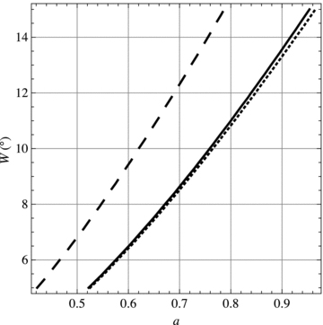
Banded magnetic field stability diagram. For banded profiles of the form (equation 29), with strength a, width W and central position μ=d= sin(latitude), instability can only occur at points (a, W) to the right-hand side of the relevant curve for each latitude. Full curve: 30° latitude bands; dashed curve: 15° latitude; dotted curve: 45° latitude.

Open in new tabDownload slide

5.1 Role of k

The generalized eigenvalue problem (equation 29) is easily converted into the standard eigenvalue problem

31

where and ⁠. In the k→∞ limit, reduces to ⁠.

Clearly, σ²=N² at k= 0. But what happens to the eigenvalues as k increases from 0 to ∞ or as the magnetic field or rotation strengthens? We perform an analysis which makes it clear that how σ asymptotically approach the eigenvalues of as k→∞.

First, we perform the Jordan decomposition ⁠. In the usual case where there are no degenerate eigenvalues, is diagonal and contains those eigenvalues as its elements. Irrespective of this, may be substituted into equation (31), which is then re-arranged to yield

32

where

33

is the identity matrix and ⁠. Clearly, as k→∞, indicating diagonal dominance for large k, and similar quadratic convergence to the eigenvalues of (elements of the diagonal matrix ⁠). This follows from Gerschgorin's theorem, as the off-diagonal terms are all ⁠.

In Fig. 2, we address the k dependence of a banded profile. The unstable eigenvalues are apparent. Interestingly, there appear to be two distinct families of eigenmode; one closely bound to the buoyancy frequency and one (much sparser) which seems independent of it once k becomes large enough.

Figure 2

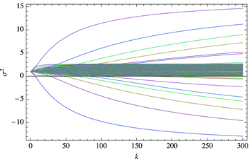
Symmetric eigenvalues σ² as functions of k for the banded case ω₀= 1 −0.18μ², a= 2 magnetic bands of width 5° centred at μ= 0.5, N= 1. Here, 201 expansion modes are used to adequately resolve the narrow magnetic band.

Open in new tabDownload slide

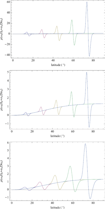
Fig. 3 illustrates the eigenfunctions of unstable modes as k increases. We see that they become much more narrowly confined to the unstable region on the poleward shoulder of the band. We conclude that magnetic bands in the radiative zone, and also perhaps in an overshoot layer, are extremely susceptible to axisymmetric instabilities sharply localized on their poleward shoulders. This illustrates how the right-hand side of equation (15) becomes negative by concentrating the eigenfunction where ⁠. Experiment suggests that, irrespective of N, instability always results at sufficiently large k if is negative somewhere.

Figure 3

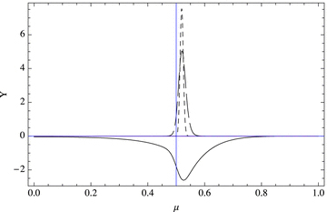
The eigenfunctions, calculated using the expansion method, corresponding to the most unstable eigenvalues σ= 0.875505 ı, 3.12112 ı and 3.70786 ı for k= 10 (full curve), 100 (long-dashed) and 500 (dashed), respectively, in the symmetric case for the banded profile of Fig. 2. The 5° magnetic band is centred on μ= 0.5, indicated by the vertical line. N= 1 throughout.

Open in new tabDownload slide

5.2 Role of N

Let us now further explore the effects of increasing N. As noted in Section 4,

34

n= 0, 1, 2, …, when σ²≫μ[(1 −μ²)α₀α′₀+ω₀Ω₀]. Consequently, we expect to see this asymptotic behaviour for large N. This is certainly the case in Fig. 4. Note how the sole unstable eigenvalue at small N is quickly overwhelmed by increasingly stable stratification. Also note that σ < N when N is large, in accordance with Corollary 4.

Figure 4

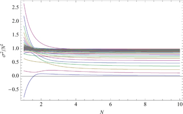
σ²/N² as a function of Brunt–Väisälä frequency N for symmetric perturbations with ω₀= 1 − 0.18μ², k= 10 and an a= 2 magnetic band at 30° latitude of width 5°. (Eigenexpansion calculation with 201 modes.)

Open in new tabDownload slide

Examination of the important case, N= 0 (convection zone), not addressed in Fig. 4 is deferred till Figs 5,10 and 11 (top panels).

Figure 5

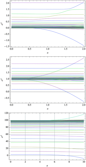
Symmetric eigenvalues σ² (k= 10) as functions of field strength parameter a for the magnetic band at 30° latitude of width 5°. Top panel: N= 0; centre panel: N= 1; bottom panel: N= 10. Note the extended range in a in the bottom panel.

Open in new tabDownload slide

Figure 10

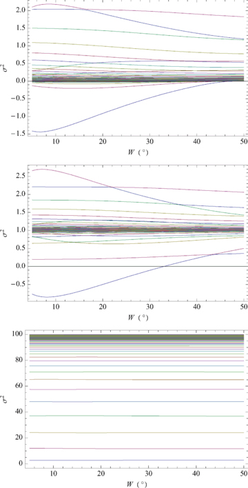
Symmetric eigenvalues σ² (k= 10) as functions of bandwidth W for the magnetic band at 30° latitude and strength a= 2. Top panel: N= 0; centre panel: N= 1; bottom panel: N= 10.

Open in new tabDownload slide

Figure 11

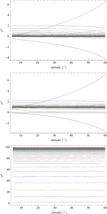
Symmetric eigenvalues σ² (k= 10) as functions of band latitude for the magnetic band of width 5° and strength a= 2. Top: N= 0; centre: N= 1; bottom: N= 10.

Open in new tabDownload slide

5.3 Role of field strength a

How do the frequencies vary with field strength a? We examine our standard 5° band at ±30°, but vary the field strength parameter a (Fig. 5). If N is small enough, increasing a gives rise to unstable eigenvalues (note the avoided crossings). However, once N becomes even moderately large (10 in the bottom panel), it suppresses all instability up till very high values of a (7.57 in this case).

5.4 Varying a, k and N: the marginal stability equation

In the radiative zone, the Brunt–Väisälä frequency is very large compared to the rotational frequency, N≫ω₀. Rotation is therefore unimportant. For the magnetic field to destabilize, the system requires a similarly large a. Fig. 7 (symmetric) indicates that instability increases linearly with a at fixed N, and that stability ensues as N increases at fixed a.

Figure 7

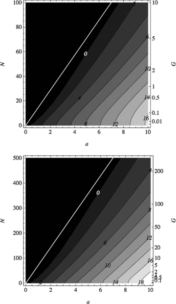
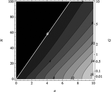
The growth rate of symmetric instabilities of the 5° band at 30° latitude with n= 1 (top panel) and n= 5 (bottom panel) as a function of field strength a and dimensionless Brunt–Väisälä frequency N (or effective gravity G). The differential rotation ω₀= 1 − 0.18μ² has been re-introduced. The black region corresponds to stability and the white line to the asymptotic curve (see text). For this magnetic profile, ⁠.

Open in new tabDownload slide

Let us now neglect rotation and explore the exchange of stabilities. This occurs when σ= 0, in which case equation (13) becomes

35

where α₀=aA₀ and

36

Here, A₀(μ) defines the band shape, assumed fixed, and a its strength. Any eigenvalue ν of equation (35), together with the usual boundary conditions, corresponds to a marginally stable case σ= 0. We define ν₀ to be the smallest positive eigenvalue of equation (35).2

Theorem 3

In the ω₀≪N limit, any triple (a, k, N) corresponding to marginal stability σ= 0 remains marginally stable as a, k and N are adjusted, provided ak/N stays fixed. Furthermore, for a given a and N, the minimum unstable k is ⁠.

Fig. 6 confirms this. It shows that is correct; the stability margin of a case without rotation lies exactly on the expected line.

Figure 6

The growth rate (labelled contours) of symmetric instabilities of the 5° band at 30° latitude with n= 1 (k= 99.3459) in the absence of rotation, presented as a function of field strength a and Brunt–Väisälä frequency N. The asymptotic marginal stability curve (in white), corresponding to ⁠, is exact in this instance. The black region is stable.

Open in new tabDownload slide

For future comparison with the HPE approach of Dikpati et al. (in preparation), we set k=nπ/H, where is the layer thickness (recall that the Boussinesq shell has radius r= 1). Here, n is an integer specifying the number of half wavelengths which fit across the layer. With this H, our Brunt–Väisälä frequency N and their ‘effective gravity’G are related by G=N²H²= 10⁻³N². We look at both n= 1 (k= 99.3459) and n= 5 (k= 496.729).

Fig. 7 (top panel) adds rotation. As expected, its stabilizing influence shifts the marginal stability curve slightly to the right-hand side. In the bottom panel, k is increased by a factor of 5, but the theoretical marginal stability line remains equally valid.

Fig. 8 similarly plots as a function of k (or n) and N for a fixed. The top panel has no rotation, and again, the marginal stability line is exact. The bottom panels re-introduce our standard differential rotation for a= 1 and 4. Note that the rotationless marginal stability curve again provides a good estimate of where instability turns on with rotation present, provided a is large. For smaller a, where rotation is more important (recall we are comparing with ω₀Ω₀), the discrepancy is large.

Figure 8

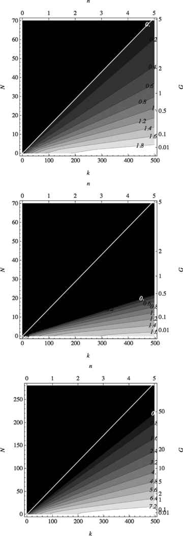
The growth rate of symmetric instabilities of the 5° band at 30° latitude. Top panel: a= 1, no rotation; middle panel: a= 1 with rotation; bottom panel: a= 4 with rotation, all as functions of k (or n) and N (or G). Note the higher growth rate at higher a. The differential rotation ω₀= 1 − 0.18μ² is employed for the bottom panels. The black region corresponds to stability and the white line to the asymptotic exchange of stability curve ⁠, which is exact in the non-rotating case. For this magnetic profile, ⁠.

Open in new tabDownload slide

Fig. 9 plots as a function of bandwidth and latitude. In both the symmetric and the antisymmetric cases, the minimum is around 5, though this occurs for wide low-latitude bands in the symmetric case, and for narrower high-latitude bands in the antisymmetric case. The minimum in the symmetric case is 4.976 at W= 35.1° and latitude 16.7°. The antisymmetric case has a minimum within the domain displayed in Fig. 9 of 5.312 at W= 11° and latitude 60°, but continues to decrease at higher latitudes.

Figure 9

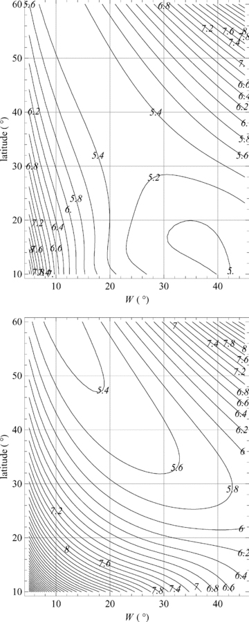
The asymptotic factor (labelled contours) determining the minimum unstable radial wavenumber for given N and a in the absence of rotation for bands of width W and a range of latitudes. Top panel: symmetric case; bottom panel: antisymmetric case.

Open in new tabDownload slide

5.5 Role of bandwidth W

Fig. 10 shows reducing instability with increasing bandwidth at fixed a and latitude, as expected because of the increase in on the poleward shoulders (Corollary 2). Again, σ < N when N is large (see Corollary 4).

5.6 Role of band latitude

Fig. 11 shows increasing instability with increasing band latitude at a= 2 and small N. This is again expected: Fig. 12(a) shows how attains larger and larger negative values on the poleward shoulder as band latitude is increased (cf. Corollary 2). The lower panels of Fig. 12 demonstrate that the bands are stable at even slightly lower field strengths a, as previously seen in Fig. 5 and as predicted in Fig. 1.

Figure 12

as a function of latitude for bands at 15°, 30°, 45°, 60° and 75°. Top panel: a= 2, W= 5°; centre panel: a= 0.5, W= 5°; bottom panel: a= 0.75, W= 10°. Negative values (on the poleward shoulders) are a destabilizing influence (Corollary 2). The rotational angular velocity is ω₀= 1 − 0.18μ² as usual. The relative roles of rotation (the slow rise) and magnetic field (the banded differentiated Gaussians) are readily distinguished. Corollary 2 indicates stability of 5° mid-latitude bands for a≲ 0.5 and N²≥ 0 and of 10° mid-latitude bands for a≲ 0.75 and N²≥ 0.

Open in new tabDownload slide

5.7 Visualization

Fig. 13 depicts the development of an m= 0 band instability at k= 30. Of course, arbitrarily higher k are even more unstable (slightly) and result in finer kinked structure in r, unless dissipative effects limit them. As expected, the effect is predominantly on the poleward shoulder of the band.

Figure 13

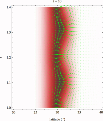
Linear development of the k= 30 symmetric instability in latitude–radius space of the 5°, a= 1 band at 30° latitude with N= 1. The shading represents (toroidal) magnetic field strength (field direction into the page) and the arrows represent velocity (by both their length and colour saturation). The eigenvalue is σ= 0.538 ı. The eigenfunction is displayed at time t= 10, given an initial perturbation of 0.1 per cent at t= 0.

Open in new tabDownload slide

Figs 14 and 15 illustrate symmetric and antisymmetric instabilities, respectively, in 10° bands at 15° latitude. In the symmetric case with a= 4, the eigenfunction ties together strongly across the equator, resulting in a significantly different eigenvalue for the symmetric (0.955 ı) and antisymmetric (0.708 ı) cases. Although the magnetic bands remain distinctly confined to their respective hemispheres at the epoch shown, the velocity clearly crosses the equator vigorously. Note also that the high Brunt–Väisälä frequency causes the velocity cells to be almost entirely latitudinal, as radial motion against the stratification is very difficult. In the antisymmetric case, the velocity equatorward of the band is weak.

Figure 14

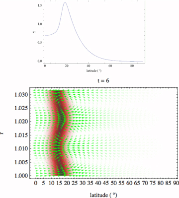
High stratification case N= 100 and n= 3 (k= 3π/H with ⁠) for an a= 4, 10° band at 15° latitude. Symmetric case. Top panel: the eigenfunction. Note the large value at the equator. Bottom panel: linear development of the instability (note that the vertical axis has been expanded to aid visibility). The eigenvalue is σ= 0.955 ı.

Open in new tabDownload slide

Figure 15

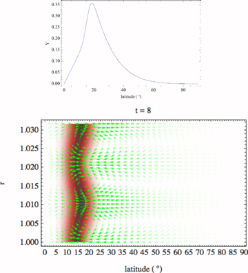
Same as Fig. 14, except for the antisymmetric case. The eigenvalue is σ= 0.708 ı.

Open in new tabDownload slide

For a high latitude (45°) band (not shown), the eigenfunction indicates that the coupling across the equator is much reduced. This is also suggested by the fact that the symmetric and antisymmetric eigenvalues are the same to seven decimal places, and by greatly reduced equatorial velocities.

6 CONCLUSIONS

We draw the following conclusions about m= 0 instabilities in the Boussinesq approximation.

• σ² is real, so there is no overstability.

• Stratification is a stabilizing influence if N² > 0 and destabilizing if N² < 0.

• Standard solar differential rotation ω₀= 1 −sμ², 0 < s < 1, is a stabilizing influence.

• Classical broad magnetic profiles are stabilizing, but banded profiles are destabilizing on their poleward shoulders, where μα₀α′₀ < 0.

• Banded magnetic profiles are stable up to some magnetic field threshold a≈ 0.4–1 which depends on bandwidth and latitude (Fig. 1).

• If anywhere, there will always be unstable modes at sufficiently high k. Increasing N² delays but does not ultimately suppress this. Diffusive effects could limit high-k instability, but we have not explored these (though see Paper I for a discussion of how thermal conduction affects the non-axisymmetric instabilities).

• The eigenfunctions of unstable modes in banded magnetic cases are more sharply confined to the poleward shoulder of the bands as k increases, but less tightly confined as N increases.

• In the absence of rotation, the marginal stability case σ= 0 corresponds to ⁠, where ν₀ depends only on the shape of the band and not its strength. For the classical Gaussian bands discussed here, Fig. 9 presents contour plots of for a range of bandwidth W and band latitude. Typically, is around 5–7 for cases of solar interest. Re-introducing rotation slightly stabilizes this, moving the critical wavenumber slightly above k_min (assuming a is large; the effect of rotation is more significant if a≲ 1; see Fig. 8).

• is an important quantity for band instability: the larger it is (above ⁠), the larger the growth rate.

• The velocity produced by axisymmetric instabilities at large N in low-latitude bands couples across the equator, setting up shallow meridional flows extending well beyond the bands.

7 DISCUSSION ON THE SIGNIFICANCE OF INSTABILITY IN BANDS

At first sight, the prevalence and vigour of both m= 0 and m= 1 high radial wavenumber instabilities present a challenge to the idea that sufficient toroidal magnetic flux can be stored and amplified in the tachocline to supply the solar cycle. As noted in Paper I, it would appear that toroidal fields of the order of 10 T (10⁵G) are needed for this purpose if storage is entirely in the convective overshoot layer, or somewhat less if the magnetic field extends deeper into the radiative zone proper. Such high field strengths are also required to maintain the integrity of rising flux tubes destined to form active regions at the surface (e.g. Moreno-Insertis, Caligari & Schüssler 1995) and to ensure that they do not appear at too high latitudes (Choudhuri & Gilman 1987). The axisymmetric stability limits on field strength in banded toroidal fields are summarized in Fig. 1, and at least approach these required values.

However, non-axisymmetric instabilities can set in at much lower field strengths. This is illustrated in Fig. 16, where both the m= 0 and 1 growth rates are plotted as a function of a for a typical banded profile (see caption for details) at k= 1000 (the large k delivers a near maximal growth rate).3 The axisymmetric case is strictly stable up to a= 0.76 for N= 0, but the m= 1 modes are weakly unstable throughout. With mild stabilizing stratification (N= 10), both m= 0 and 1 growth rates are significantly reduced. N= 100 (quite modest for the upper radiative region), corresponding to a buoyancy period of about 6 h, completely stabilizes the m= 0 modes up to a= 1.52 and reduces the m= 1 growth rates to negligible values (even at a= 1, the e-folding time is almost 4 yr). Of course, large N does nothing to stabilize the 2D tipping instabilities k= 0 and m= 1, but these typically saturate at tipping angles of 10°–20° (Cally, Dikpati & Gilman 2003) and do not disrupt the band.

Figure 16

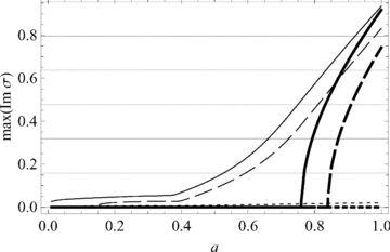
Comparison of the growth rates as a function of field strength a of the most unstable antisymmetric modes at k= 1000, and m= 0 (thick curves) and m= 1 (thin) in the case of W= 10° bands at ±30° latitude. The horizontal grid represents growth rates which produce amplitude increases of e, e², e³, …, in one equatorial rotation period (month). Full lines: N= 0; dashed: N= 10; dotted: N= 100.

Open in new tabDownload slide

Based on an analysis of instabilities in the broad magnetic profile α₀=aμ, Kitchatinov & Rüdiger (2008) argue that the high-k shredding instabilities limit radiation zone field strengths to a mere 600 G, at which point diffusive effects are able to stop them. However, as we have just seen, banded profiles are easily stabilized up to high field strengths by the stable stratification of the radiative core. Diffusive effects will limit the most unstable (high-k) instabilities further. We therefore see little impediment to storing G fields below the convection zone. It is also likely that significant twist in the flux ropes stabilizes them, as happens in rising tubes (Moreno-Insertis et al. 1996).

M.D. acknowledges partial support from NASA grants NNH05AB521 and NNX08AQ34G.

REFERENCES