Post-common envelope binaries from SDSS – III. Seven new orbital periods Free

Abstract

1 INTRODUCTION

Most of the stellar sources are formed as parts of binary or multiple systems. Therefore the study of binary star evolution represents an important part of studying stellar evolution. While the majority of the wide main-sequence binaries evolve as if they were single stars and never interact, a small fraction is believed to undergo mass transfer interactions. Once the more massive main-sequence star becomes a red giant it eventually overfills its Roche lobe. Dynamically unstable mass transfer exceeding the Eddington limit ensues on to the companion star, which consequently also overfills its own Roche lobe. The two stars then orbit inside a common envelope (CE; e.g. Paczynski 1976; Livio & Soker 1988; Iben & Livio 1993; Taam & Ricker 2006; Webbink 2007), and friction inside this envelope causes a rapid decrease of the binary separation. Orbital energy and angular momentum are extracted from the binary orbit and lead to the ejection of the envelope, exposing a post-CE binary (PCEB). After the envelope is expelled PCEBs keep on evolving towards shorter orbital periods through angular momentum loss via gravitational radiation and, for companion stars above the fully convective mass limit, by magnetic wind braking. In binaries that do not undergo a CE phase both components evolve almost like single stars and keep their wide binary separations. A predicted consequence is hence a strongly bimodal binary separation and orbital period distribution among post-main-sequence binaries, with PCEBs concentrated at short orbital periods, and non-PCEBs at long orbital periods.

The scenario outlined above is thought to be a fundamental formation channel for a wide range of astronomical objects such as low-mass X-ray binaries, double degenerate white dwarfs, neutron star binaries, cataclysmic variables (CVs) and supersoft X-ray sources. Some of these objects will eventually end their lives as type Ia supernovae and short gamma-ray bursts, which are of great importance for cosmological studies.

While the basic scenario of CE evolution has been known for a long time (e.g. Paczynski 1976), the physical details involved are complex and still poorly understood. As a result, full hydrodynamical models for the CE phase have been calculated only for a small number of cases (Sandquist, Taam & Burkert 2000; Ricker & Taam 2008). Similarly, orbital evolution through magnetic braking is not well understood, with different prescriptions in angular momentum loss differing by orders of magnitudes (e.g. Verbunt & Zwaan 1981; Andronov, Pinsonneault & Sills 2003). Consequently, current binary population synthesis models still have to rely on simple parametrizations of energy or angular momentum equations (Dewi & Tauris 2000; Nelemans et al. 2000; Nelemans & Tout 2005; Politano & Weiler 2006, 2007).

A fundamental problem in advancing our understanding of CE evolution and magnetic braking in close binaries is the shortage of stringent observational constraints that can be used to test and calibrate the theory. PCEBs consisting of a white dwarf and a main-sequence star are a very well-suited class of objects to provide the required innovative observational input since they are numerous, well understood in terms of their stellar components, they are bright and hence accessible with 2–8 m telescopes, and their study is not complicated by mass transfer. Schreiber & Gänsicke (2003) analysed a sample of 30 well-studied PCEBs and showed that the population of PCEBs known so far is not only small but also heavily biased towards young systems with low-mass secondary stars, and can hence not be used for comparison with population models (e.g. Willems & Kolb 2004).

The Sloan Digital Sky Survey (York et al. 2000; Stoughton et al. 2002; Adelman-McCarthy et al. 2008, SDSS) is currently dramatically increasing the number of known white dwarf plus main-sequence (WDMS) binaries (Schreiber, Nebot Gomez-Moran & Schwope 2007; Silvestri et al. 2007), paving the way for large-scale observational PCEB population studies. We have initiated an observational programme to identify the PCEBs among the SDSS WDMS binaries, and to determine their binary parameters (Rebassa-Mansergas et al. 2007; Schreiber et al. 2008). Those systems in which significant radial velocity variation is detected are classified as close binaries or PCEBs. Here we present follow-up observations of 11 PCEB candidates identified in Rebassa-Mansergas et al. (2007) and provide accurate values of the orbital periods as well as estimates of their stellar parameters and orbital inclinations for seven of these systems.

2 OBSERVATIONS

We have obtained time-resolved spectroscopy and photometry for 11 SDSS WDMS binaries (Table 1, Fig. 1), henceforth designated SDSS J0052−0053, SDSS J0246+0041, SDSS J0309−0101, SDSS J0820+4314, SDSS J0314−0111, SDSS J1138−0011, SDSS J1151−0007, SDSS J1529+0020, SDSS J1724+5620, SDSS J2241+0027 and SDSS J2339−0020. Below we briefly describe the instrumentation used for the observations, and outline the reduction of the data.

Figure 1

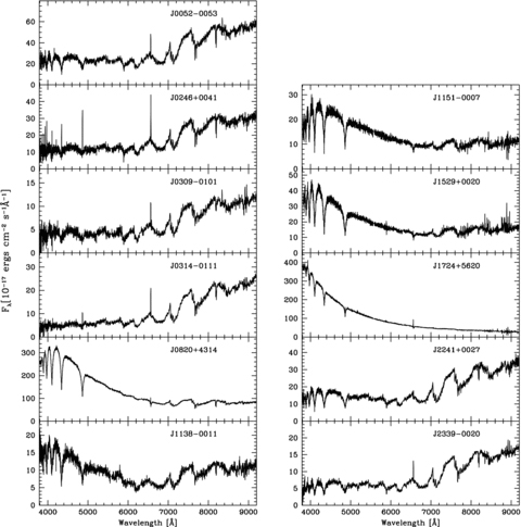
SDSS spectra of the 11 SDSS white dwarf main-sequence binaries studied in this paper.

Open in new tabDownload slide

2.1 Spectroscopy

• Magellan Baade: Intermediate-resolution long-slit spectroscopy of SDSS J0314−0111 and SDSS J2241+0027 was obtained on the nights of 2007 October 2 and 3 using the IMACS imaging spectrograph attached to the Magellan Baade telescope at Las Campanas Observatory. The 600 ℓ mm⁻¹ red-sensitive grating was used along with the slit-view camera and a slit width of 0.75 arcsec, giving a reciprocal dispersion of 0.39 Å px⁻¹. The IMACS detector is a mosaic of eight 2000 × 4000 SITe CCDs, and long-slit spectra with this instrument are spread over the short axis of four of these CCDs. Using a grating tilt of 14°.7 allowed us to position the Na i λλ8183.27, 8194.81 doublet towards the centre of CCD2 and the Hα line near the centre of CCD4.

  The images were reduced using starlink software, and the pamela and molly packages (Marsh 1989) were employed to optimally extract and calibrate the spectra. By fitting Gaussian functions to arc and sky emission lines we find that the spectra have a resolution of approximately 1.6 Å. Helium arc lamp exposures were taken at the start of each night in order to derive a wavelength solution with a statistical uncertainty of only 0.002 Å (Marsh, Robinson & Wood 1994). This was applied to each spectrum taken on the same night. Detector flexure was measured and removed from the wavelength solution for each spectrum using the positions of sky emission lines (Southworth et al. 2006; Schreiber et al. 2008). Flux calibration and telluric line removal was performed using molly and spectra of the standard star BD +28°4211.

• Magellan Clay and Very Large Telescope (VLT): The observations of SDSS J1138-0011, SDSS J1151−0007 and SDSS J1529+0020 were obtained with the same set-up and reduced in the same manner as described by Schreiber et al. (2008), and we refer the reader to that paper for full details.

• New Technology Telescope (NTT): Two observing runs were carried out at the NTT in 2007 August and October, providing intermediate time-resolved spectroscopy of SDSS J0052−0053, SDSS J0246+0041, SDSS J0309−0101, SDSS J2241+0027 and SDSS J2339−0020. We used the EMMI spectrograph equipped with the Grat#7 grating, the MIT/LL red mosaic detector, and a 1 arcsec wide long-slit, resulting in a wavelength coverage of λ7770– 8830 Å. The data were bias-corrected and flat-fielded using the starlink software, and spectra were optimally extracted using the pamela package. Helium–agon arc lamp spectra were taken at the beginning of each night and were then used to establish a generic pixel–wavelength relation using molly. Specifically, we fitted a fourth-order polynomial which gave rms smaller than 0.02 Å for all spectra. We then used the night sky emission lines to adjust the zero-point of the wavelength calibration, thus correcting for instrument flexure. The spectral resolution of our instrumental set-up determined from the sky lines is 2.8 Å. Finally, the spectra were calibrated and corrected for telluric absorption within molly using observations of the standard star Feige 110.

• William Herschel Telescope (WHT): One spectrum of SDSS J1138−0011 was taken with the 4.2-m WHT in 2007 June at the Roque de los Muchachos observatory on La Palma. The double-beam ISIS spectrograph was equipped with the R158R and the R300B gratings, and a 1 arcsec long slit, providing a wavelength coverage of λ7600– 9000 Å. The spectral resolution measured from the sky lines is 1.6 Å. Reduction and calibration were carried in the same way as described for the NTT above.

• SDSS: For one system, SDSS J1724+5620, we were able to determine an accurate orbital period from our photometry alone, but were lacking follow-up spectroscopy. SDSS DR6 contains three 1-d calibrated spectra for SDSS J1724+5620 (MJD-PLT-FIB 51813−357−579, 51818−358−318 and 51997−367−564). Each of these spectra is combined from at least three individual exposures of 900 s, which are also individually released as part of DR6.1 For SDSS J1724+5620, a total of 23 subspectra are available, of which 22 allowed reliable radial velocity measurements.

2.2 Photometry

• IAC80 and AIP 70-cm telescopes: We obtained differential photometry of SDSS J1724+5620 with the IAC80 telescope at the Observatorio del Teide (Spain) and the 70-cm telescope of the Astrophysical Institute of Postdam at Babelsberg (Germany) for a total of 13 nights during 2006 May, August and September and 2007 March. The IAC 80-cm telescope was equipped with a 2000 × 2000 CCD. A binning factor of 2 was applied in both spatial directions and only a region of 270 × 270 (binned) pixels of size 0.66 arcsec was read. The detector used at the Babelsberg 70-cm telescope was a cryogenic 1000 × 1000 Tek CCD. The whole frame was read with a binning factor of 3, resulting in a scale of 1.41 arcsec pixel⁻¹. A semi-automated pipeline involving dophot was used to reduce the images and extract the photometric information.

• Calar Alto 2.2-m telescope: We used CAFOS with the SITe 2000 × 2000 pixel CCD camera on the 2.2-m telescope at the Calar Alto observatory to obtain filterless differential photometry of SDSS J0314−0111. Only a small part of the CCD was read out in order to improve the time resolution. The data were reduced using the pipeline described in Gänsicke et al. (2004), which pre-processes the raw images in midas and extracts aperture photometry using the sextractor (Bertin & Arnouts 1996).

• Kryoneri 1.2-m telescope: Filterless photometry of SDSS J0820+4311 was obtained in 2006 November at the 1.2-m Kryoneri telescope using a Photometrics SI-502 516 × 516 pixel camera. The data reduction was carried out in the same way as described above for the Calar Alto observations.

3 ORBITAL PERIODS

3.1 Radial velocities

In Rebassa-Mansergas et al. (2007) we measured the radial velocities fitting a second-order polynomial plus a double-Gaussian line profile of fixed separation to the Na i λλ8183.27, 8194.81 absorption doublet. Free parameters were the amplitude and the width of each Gaussian and the radial velocity of the combined doublet. Here we adopt a slightly modified approach, using just a single width parameter for both line components. This reduction in the number of free parameters increases the robustness of the fits. Radial velocities measured in this way for nine WDMS binaries are given in Table 2. In addition, we measured the companion star radial velocities for SDSS J1724+5620 by means of a Gaussian fit to the Hα emission line clearly visible in 22 of the SDSS subexposures (Section 2.1), which are also reported in Table 2.

Scargle (1982) periodograms calculated from the radial velocities of each system to investigate the periodic nature of the velocity variations contain a number of aliases due to the sampling pattern of the observations (Fig. 2, left-hand panel). We carried out sine fits of the form

1

to the velocity data sets of each system, where γ is the systemic velocity, K_sec is the radial velocity semi-amplitude of the companion star, T₀ is the time of inferior conjunction of the secondary star, and P_orb is the orbital period. Several fits were done, adopting the frequencies corresponding to the strongest peaks in the power spectra as initial conditions. The parameters resulting from these fits are reported in Table 3. For SDSS J0052−0053, SDSS J0246+0041, SDSS J0314−0111, SDSS1151−0007, SDSS J1529+0020 and SDSS J2339−0020 the sine fits allow a unique choice of the orbital period. For SDSS J1724+5620, the sampling of the SDSS spectra is very sparse, resulting in finely structured aliases superimposed on a sequence of large aliases spaced by 1 d⁻¹. A sine fit to the radial velocities started off at the 3 d⁻¹ alias provides a spectroscopic orbital period of 7.992 43(16) h, which is consistent with the more accurate value determined from the photometry (Section 3.2). The radial velocity data for all seven systems folded over their orbital periods are shown in Fig. 2 (right-hand panel).

Figure 2

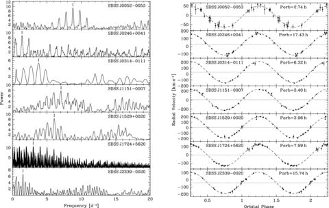
Left-hand panel: Scargle periodograms calculated from the radial velocity variations measured from the Na i absorption doublet in SDSS J0052−0053, SDSS J0246+0041, SDSS J0314−0111, SDSS J1151−0007, SDSS J1529+0020 and SDSS J2339−0020, and from the Hα emission line in SDSS J1724+5620. The aliases with the highest power are indicated by tick marks. Right-hand panel: the radial velocity measurements folded over the orbital periods of the systems, as determined from the best sine fits (Table 3).

Open in new tabDownload slide

The periodograms calculated from the radial velocity measurements of the PCEB candidates SDSS J0309−0101, SDSS J1138−0011 and SDSS J2241+0027 do not reveal any significant peak. The low amplitude of the radial velocity variations observed in these three objects suggests that they may be wide WDMS binaries rather than PCEBs. This issue will be discussed further in Section 5.3.

3.2 Light curves

The light curves of SDSS J0314−0111 and SDSS J1724+5620 display variability with an amplitude of ∼0.05 and 0.1 mag, respectively. We calculated periodograms for both systems using the ORT/TSA command in midas, which folds and phase-bins the data using a grid of trial periods and fits a series of Fourier terms to the folded light curve (Schwarzenberg-Czerny 1996).

A strong peak is found in the periodogram of SDSS J0314−0111 at 3.8 d⁻¹, i.e. 6.3 h (Fig. 3, top left-hand panel). Folding the photometric data over that period results in a double-humped modulation which we identify as ellipsoidal modulation (Fig. 3, middle left-hand panel). The detection of ellipsoidal modulation indicates that the companion star must be filling a significant amount of its Roche lobe radius and have a moderately high inclination, both of which hypothesis are confirmed below in Section 4. The two minima differ in depth, as expected for ellipsoidal modulation because of the stronger gravity darkening on the hemisphere facing the white dwarf. The two maxima are also unequal, which is observed relatively often in PCEBs, and thought to be related to the presence of star spots (e.g. Kawka & Vennes 2003; Tappert et al. 2007). We conclude that the strongest periodicity detected in the photometry of SDSS J0314−0111 is consistent with the spectroscopic orbital period (Table 3). As the radial velocities span a longer temporal baseline than the photometry, they provide the more accurate period measurement, and we adopt P_orb= 6.319 ± 0.015 h for SDSS J0314−0111.

Figure 3

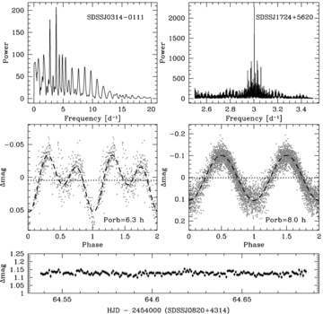
Top and middle panels: ORT periodograms and light curves folded on strongest photometric periodicities, P_orb= 6.32 ± 0.02 h for SDSS J0314−0111 and P_orb= 7.992 46 ± 0.000 03 h for SDSS J1724+5620. Bottom panel: the light curve of SDSS J0820+4314 is essentially flat, and a periodogram calculated from these data does not contain any significant periodicity.

Open in new tabDownload slide

For the analysis of SDSS J1724+5620 we separately merged the data for the R and I bands, normalized both data sets to their respective mean values, and finally combined all data into a single data set. The ORT periodogram calculated from the full light curve displays a strong signal at 3 d⁻¹, with weak aliases related to the sampling pattern inherent to the data (Fig. 3, top right-hand panel). Given the large quasi-sinusoidal shape of the modulation, and the high effective temperature of the white dwarf (Table 4), we identify the observed photometric variability as being due to heating effect (or reflection effect as it is often referred to in the literature). A sine fit to the combined data (dashed line) provided the following photometric ephemeris:

2

where φ= 0 refers to the occurrence of minimum light. The photometric period of 8 h is consistent with the alias pattern in the periodogram calculated from the Hα radial velocity variations (Fig. 2, left-hand panel). The phase-folded light curve using the photometric period is shown on the middle right-hand panel of Fig. 3. Based on the above ephemeris, the accumulated phase error for the first SDSS subspectrum (Table 2) is 0.024 cycles, which is sufficiently good to phase the radial velocities obtained from the SDSS spectra with equation (2). The phase-folded light curve and radial velocity curve are shown in Fig. 4. The phase offset between the two curves is 0.226 ± 0.005, which is consistent with ≃0.25 within the error of the fit and the ephemeris. A 0.25 phase offset is what is expected from the assumption that the photometric modulation is related to a heating effect, i.e. maximum light and red-to-blue crossing of the radial velocity corresponds to the superior conjunction of the secondary star, whereas minimum light and blue-to-red crossing of the radial velocity corresponds to its inferior conjunction.

Figure 4

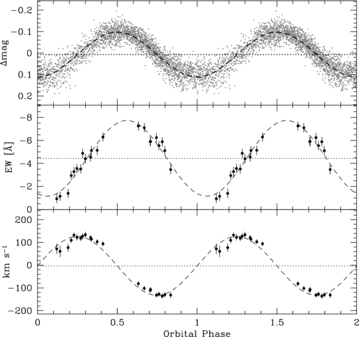
Top panel: the IAC 80 and AIP 70-cm photometry of SDSS J1724+5620 folded over the photometric period of 7.992 4632 ± 0.000 0312 h. Middle panel: the equivalent width variation of the Hα emission line measured from the SDSS spectra of SDSS J1724+5620 (Table 2) folded over the photometric period. Maximum equivalent width occur roughly in phase with the maximum in the light curve (see Section 5.2 for details). Bottom panel: the radial velocity variation of the Hα emission line. The relative phasing with respect to the photometry is consistent with the photometric modulation being caused by irradiation of the secondary star by the hot white dwarf.

Open in new tabDownload slide

Finally, we show in the bottom panel of Fig. 3 a 3.5-h light curve of SDSS J0820+4314. We monitored the system through a total of 8.2 h on three different nights (see Table 1), and found no significant photometric modulation. This implies that the companion star is significantly underfilling its Roche lobe and/or that the binary inclination is very low. The orbital period of the system will hence need to be measured from a radial velocity study.

4 BINARY PARAMETERS

In Rebassa-Mansergas et al. (2007) we developed a spectral decomposing/fitting technique for the analysis of WDMS binaries with SDSS spectroscopy. In brief, this analysis determines the white dwarf effective temperature, surface gravity, mass and radius, the spectral type and radius of the main-sequence companion, as well as two independent distance estimates based on the properties of the two stellar components. Given that the SDSS spectra reduction pipeline has been improved with DR6 (Adelman-McCarthy et al. 2008), we have re-analysed here the seven PCEBs for which we were able to determine orbital periods. Comparison with the results from DR5 reported in Rebassa-Mansergas et al. (2007) shows that the fit parameters differ slightly, but agree in the vast majority of cases within the errors. We report the average stellar parameters determined from fits to the multiple SDSS spectra in Table 4. Rewriting Kepler's third law (assuming common notation),

3

as

4

and adopting the orbital period determined from the analysis of the radial velocities and the photometry, as well as the masses from the analysis of the SDSS spectra, we are now able to estimate the orbital inclinations for the seven systems in Table 4. Two systems require some additional notes: SDSS J0314−0111 contains a DC white dwarf, and hence no white dwarf parameters could be determined from the spectral analysis, and we assume M_wd= 0.65 M_⊙ for the estimate of the inclination. In SDSS J1724+5620 the hot white dwarf is irradiating the companion star, and the implications are discussed in more detail in Section 5.2.

Inspecting equation (4), it is clear that the dominant uncertainties in the inclination estimates are only M_wd and M_sec, as the orbital periods and K_sec velocities are accurately determined. The primary uncertainty in the inclination estimates is M_sec, as it is based on the spectral type of the companion star, adopting the spectral type–mass–radius relation given by Rebassa-Mansergas et al. (2007). M_wd is determined from fitting the Balmer line profiles, and relatively well constrained. Given that sin i∝M^2/3_sec, but sin i∝M_wd, the relative weight of the uncertainty in M_sec is alleviated. We estimate the uncertainties on the binary inclinations in Table 4 by assuming in equation (4) the range in M_sec implied by a spectral type uncertainty of ±0.5 spectral classes plus the associated errors in the spectral type–mass relation, as well as the range in M_wd resulting from the Balmer line profile fits. Given the high estimate for the binary inclination, SDSS J1529+0020 is a good candidate for photometric follow-up observations probing for eclipses in its light curve.

In addition, knowing that M_sec/M_wd=K_wd/K_sec=q, we can also estimate the expected orbital velocity of the white dwarf K_wd (Table 4). The predicted K_wd amplitudes could easily be measured, e.g. using Hubble Space Telescope/COS observations, and such measurements would be very valuable to improve the overall constraints on the system parameters of these PCEBs. Finally, we can estimate the orbital separations and Roche lobe radii of the secondary stars from Kepler's third law and Eggleton's (1983) expression

5

5 NOTES ON INDIVIDUAL SYSTEMS

5.1 SDSS J0052−0053, a detached CV in the period gap?

SDSS J0052−0053 has the shortest orbital period, the smallest radial velocity amplitude, and lowest inclination in our sample (Fig. 2, Table 4). Another intriguing feature of SDSS J0052−0053 is that the Roche lobe secondary radius and the secondary star radius overlap within the errors (see Table 4). The SDSS and Magellan spectra certainly rule out ongoing mass transfer, i.e. that SDSS J0052−0053 is a disguised CV. Two possible scenarios could apply to the system. SDSS J0052−0053 could be either be a pre-CV that is close to develop in a semidetached configuration, or it could be a detached CV in the 2–3 h period gap. Standard evolution models based on the disrupted magnetic braking scenario (e.g. Rappaport, Joss & Verbunt 1983; Kolb 1993; Howell, Nelson & Rappaport 2001) predict that CVs stop mass transfer and the secondary star shrinks below its Roche lobe radius once they evolve down to P_orb≃ 3 h. Subsequently, these detached CVs evolve through the period gap, until the companion star fills its Roche lobe again at P_orb≃ 2 h. Population models based on the disrupted magnetic braking hypothesis predict that the ratio of detached CVs to pre-CVs (with appropriate companion star masses to (re-)initiate mass transfer at P_orb≃ 2 h) should be ≳4 (Davis et al. 2008), hence a substantial number of such systems is expected to exist. So far, only one other system with similar properties is known, HS 2237+8154 (Gänsicke et al. 2004).

5.2 SDSS J1724+5620, a PCEB with a strong heating effect

SDSS J1724+5620 contains the hottest white dwarf among our sample of PCEBs, which affects the determination of its system parameters in several ways. First, irradiation heating the inner hemisphere of the companion will cause it to appear of earlier spectral type than an unheated star of same mass. This effect is observed in the analysis of the three SDSS spectra available in DR6. The spectral decomposition types the companion star as M3-4, and combining the flux scaling factor of the M star template and the spectral type–radius relation (see Rebassa-Mansergas et al. 2007, for details) indicates an average distance of d_sec= 633 ± 144 pc. This is roughly twice the distance implied from the model fit to the residual white dwarf spectrum, d_wd= 354 ± 15 pc, indicating that the spectral type of the companion star determined from the SDSS spectrum is too early for its actual mass and radius, as expected for being heated by the white dwarf. Fixing the spectral type of the companion to M5, the spectral decomposition results in d_sec= 330 ± 150 pc, consistent with the distance based on the white dwarf fit.

An additional complication is that the radial velocity of the companion star was measured from the Hα emission line, as the Na i absorption doublet was too weak in the individual 900-s SDSS spectra. The equivalent width of the Hα emission shows a noticeable variation as a function of binary phase, with maximum equivalent with near the maximum in the light curve, indicating that the Hα emission is concentrated on the inner hemisphere of the companion star (Fig. 4). A phase offset of 0.046 ± 0.008 is observed between the photometry and the Hα equivalent width, which we attribute to systematic problems in measuring the equivalent width of the Hα embedded in the photospheric absorption line from the white dwarf, given the poor quality of the individual SDSS subspectra. As a consequence of Hα predominantly originating on the inner hemisphere of the companion star, the observed K_sec is an underestimate of the true radial velocity amplitude (e.g. Wade & Horne 1988; Orosz et al. 1999; Vennes, Thorstensen & Polomski 1999; Aungwerojwit et al. 2007). The radial velocity amplitude of the secondary star's centre of mass can be written as (Wade & Horne 1988)

6

where ΔR is the displacement of the centre of light from the centre of mass. ΔR= 0 implies that the centre of light and the centre of mass coincide, whilst ΔR=R_sec gives the maximum possible displacement. If one assumes that the irradiated emission on the secondary is distributed uniformly over the inner hemisphere, and that the contribution of the irradiation is zero on its unirradiated face, then ΔR= (4/3π)R_sec (Wade & Horne 1988; Orosz et al. 1999; Vennes et al. 1999). Assuming that the spectral type is in the range M3–5, different combinations of secondary mass and radius, and radial velocity amplitude, K_sec,corr, can then constrain the orbital parameters of SDSS J1724+5620 (Table 4).

5.3 SDSS J0309−0101, SDSS J1138−0011 and SDSS J2241+0027: wide WDMS binaries?

SDSS J0309−0101, SDSS J1138−0011 and SDSS J2241+0027 were flagged as PCEB candidates by Rebassa-Mansergas et al. (2007) on the base of a 3σ radial velocity variation in between their different SDSS spectra, as measured from either the Hα emission line or the Na i absorption doublet from the companion star. However, the additional intermediate-resolution spectra taken for these three objects (Table 1) do not show a significant radial velocity variation (Table 2, Fig. 5). It is therefore important to review the criterion that we used in our first paper to identify PCEBs from repeated SDSS spectroscopy in the light of two subtle changes.

Figure 5

SDSS radial velocities (triangles) along with the Na i radial velocities measured in this paper (solid dots) of SDSS J0309−0101, SDSS J1138−0011 and SDSS J2241+0027. The data at hand suggest that these three systems are wide WDMS binaries instead of PCEBs.

Open in new tabDownload slide

On the one hand, we have slightly modified the procedure to fit the Na i absorption doublet, as outlined in Section 3.1. By comparing the Na i DR5 radial velocities in Rebassa-Mansergas et al. (2007) with those obtained with the new procedure for the same spectra, we find an average difference of 5 km s⁻¹ with a maximum difference of 10.5 km s⁻¹. In all cases the measurements agree within the errors.

On the other hand, we were using DR5 spectra in Rebassa-Mansergas et al. (2007), but the analysis carried out here was done using DR6 spectra, which were processed with a different reduction pipeline (Adelman-McCarthy et al. 2008). A comparison between the DR5 and DR6 radial velocity values obtained in Rebassa-Mansergas et al. (2007) and in this paper, respectively (both measured following our new procedure) provides in this case an average difference of 6.5 km s⁻¹, with a maximum of 22 km s⁻¹. Again, the radial velocity measurements agree, with the exception of a single spectrum, within the errors.

The conclusion from comparing our two methods, and the two SDSS data releases, is that the radial velocity measurements obtained are in general consistent within their errors. However, the offsets can be sufficient to move a given system either way across our criterion to identify PCEB candidates, being defined a 3σ radial variation between their SDSS spectra. This is specifically the case for systems with either low-amplitude radial velocity variations, or faint systems with noisy spectra. An additional note concerns the use of the Hα line as probe for radial velocity variations. Rebassa-Mansergas et al. (2007) identified SDSS J2241+0027 as a PCEB candidate on the basis of a large change in the Hα radial velocity between the two available SDSS spectra. However, the velocities obtained from the Na i doublet did not differ significantly. Inspecting the spectra again confirms the results of Rebassa-Mansergas et al. (2007). This suggests that the absorption lines from the secondary star are a more robust probe of its radial velocity.

A somewhat speculative explanation for the shifts found from Hα radial velocity measurements is that the main-sequence star is relatively rapidly rotating, and that the Hα emission is patchy over its surface. A nice example of a this effect is the rapidly rotating (P= 0.459 d) active M-dwarf EY Dra, which displays Hα radial velocity variations with a peak-to-peak amplitude of ∼100 km s⁻¹ (Eibe 1998). In order to explain the Hα radial velocity shifts of a few 10 km s⁻¹ observed in e.g. SDSS J2241+0027, the companion star should be rotating with a period of ∼1 d. According to Cardini & Cassatella (2007), low-mass stars such as the companions in our PCEBs that are a few Gyr old are expected to have rotational periods of the order of tens of days, which is far too long to cause a significant Hα radial velocity variation at the spectral resolution of the SDSS spectra. However, Cardini & Cassatella's study was based on single stars, and the rotation rates of the companion stars in (wide) WDMS binaries is not well established.

6 PCEB EVOLUTION

Following Schreiber & Gäensicke (2003) we determine the cooling age and the future evolution of the new PCEBs. We assume classical and disrupted magnetic braking according to the standard theory of CV evolution (e.g. Verbunt & Zwaan 1981). We used the cooling tracks of Wood (1995) and find that most of the PCEBs left the CE about 1– 5 × 10⁸ yr ago, the only exception being SDSS J1724+5620 which appears to be much younger. The time still needed to enter the semidetached CV configuration is shorter than the Hubble time for all the systems, qualifying them as representatives for the progenitors of the current CV population. The numbers we obtained from the theoretical analysis are summarized in Table 5. The estimated secondary masses are generally very close to the fully convective boundary (for which we assume M_cc= 0.3 M_⊙, see however the discussion by Mullan & Macdonald 2001; Chabrier, Gallardo & Baraffe 2007 on how this mass limit may be affected by magnetic activity) and the uncertainties involved in the secondary mass determination are quite large. The predicted evolution of all systems should therefore be considered highly uncertain as it is not clear whether magnetic braking applies or not. We therefore give in Table 5 the values obtained for both scenarios. The effect of not knowing whether magnetic braking or only gravitational radiation will drive the evolution of the systems is illustrated in Fig. 6, which shows the expected post-CE evolution for SDSS J1152−0007 and SDSS J0246+0041 for both cases.

Figure 6

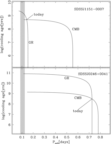
The predicted evolution of two PCEBs. The orbital period gap observed in the orbital period distribution of CVs is shaded. As the secondary masses of SDSS J1151−0007 and SDSS J0246+0041 are close to the fully convective boundary, we calculated the evolution assuming classical magnetic braking (CMB) and assuming only gravitational radiation (GR). Obviously, the calculated orbital periods at the end of the CE phase (P_CE), the evolutionary time-scale, and the expected zero-age CV orbital period (P_sd) differ significantly.

Open in new tabDownload slide

Inspecting Table 5, the case of SDSS J0052−0053 is particularly interesting. The estimated secondary radius is consistent with its Roche lobe radius and the system is supposed to be very close to the onset of mass transfer, which is reflected by t_sd= 0 within the accuracy of our calculations. Clearly, SDSS J0052−0053 may be a detached CV in the period gap, or a pre-CV that has almost completed its PCEB lifetime. To estimate the probability for SDSS J0052−0053 being either a period-gap CV or a PCEB close to entering for the first time a semidetached state, we assume a steady state binary population. In that case, the number of detached CVs in the gap should be roughly equal to the number of CVs above the gap (Kolb 1993). In addition, the number of PCEBs in the gap should be roughly equal to the number of accreting CVs in the gap. According to CV population studies (Kolb 1993), the number of detached CVs in the gap is approximately five times higher than the number of CVs in the gap and the probability for SDSS J0052−0053 being a detached CV in the gap rather than a PCEB is ∼80 per cent. This result is a simple consequence of the fact that all CVs with donor stars earlier than ∼M3 will become detached CVs in the gap while only a rather small fraction of PCEBs, i.e. those with secondary stars of spectral type ∼M3.5–M4.5, produces CVs starting mass transfer in the period gap. This is obviously only a rough estimate. A detailed population study by Davis et al. (2008) confirms that the ratio of detached CVs to pre-CVs within the CV period gap is ∼4– 13, depending on different assumptions of the CE ejection efficiency, initial mass ratio distributions, and magnetic braking laws.

7 DISCUSSION

As outlined in Section 1, despite some recent progress our understanding of the CE phase is still very limited. The classical α prescription (Webbink 1984) that is based on a simple energy equation seems to be unable to explain the observed existence of double white dwarfs with stellar components of comparable masses and rather long orbital periods (see Webbink 2007, for more details). This disagreement motivated Nelemans et al. (2000) to develop an alternative prescription based on the conservation of angular momentum, the so-called γ algorithm. Binary population synthesis codes based on the α prescription as well as those assuming the γ algorithm predict the existence of a significant number of PCEBs with orbital periods longer than a day. Using the α mechanism, Willems & Kolb (2004) calculated the expected period distribution of the present-day WDMS binaries in the Galaxy at the start of the WDMS binary phase. Their fig. 10 clearly shows that the predicted PCEB distribution peaks around P_orb∼ 1 d, but also has a long tail of systems with up to ∼100 d. The γ algorithm, on the other hand, predicts an increase of the number of PCEBs with increasing orbital period up to P_orb≳ 100 d, i.e. the γ prescription predicts the existence of even more long orbital period (P_orb > 1 d) PCEBs (see Nelemans & Tout 2005; Maxted et al. 2007).

We have measured a total number of nine orbital periods in the course of this paper and the recently published paper by Schreiber et al. (2008). All of them have short orbital periods of less than a day. Radial velocity variations are much easier to identify in short orbital period systems, so our sample is expected to be biased towards shorter orbital periods. The crucial question is whether our observational finding, the paucity of PCEBs with P_orb > 1 d, is whether the result of that bias, or whether it reflects an intrinsic feature of the PCEB population. To answer this question we performed the following analysis. First, we carried out Monte Carlo simulations similar to those presented in Schreiber et al. (2008)2 but assuming a resolution of 15 km s⁻¹, corresponding to the typical error in the radial velocity measurements from SDSS spectra. Clearly, as shown in Fig. 7, the bias towards short orbital period systems is larger due to the lower resolution of the SDSS spectra and, as a consequence, radial velocity variations in multiple SDSS spectra of systems with P_orb > 10 d are more difficult to detect. However, the probability to detect 3σ radial velocity variations for systems in the orbital period range of P_orb∼ 1–10 d still is ∼20–40 per cent. Secondly, we assumed a uniform orbital period distribution and integrated the 3σ-detection probability (lowest dotted line) for systems with P_orb≤ 1 d and those with 10 > P_orb > 1 d. In other words, we assume that there is no decrease for 10 d P_orb > 1 d and calculate the total detection probability for 10 > P_orb > 1 d and P_orb≤ 1 d. We find that if there was indeed no decrease, the fraction of PCEBs with P_orb > 1 d in our sample should be ∼84 per cent and the number of PCEBs with P_orb > 1 d among our nine systems should be ∼ 7.6 ± 2.8. The result of our observations, i.e. no system with P_orb > 1 d among nine PCEBs disagrees with the hypothesis (i.e. there is no decrease) by 2.7σ. This indicates that the measured lack of PCEBs with P_orb > 1 d might indeed be a feature of the intrinsic population of PCEBs.

Figure 7

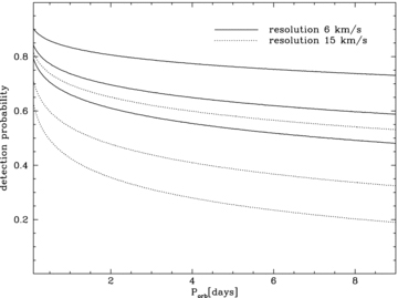
Monte Carlo simulations of the detection probability of significant radial velocity variations assuming measurement accuracy of 6 km s⁻¹, corresponding to our previous VLT/FORS observations (Schreiber et al. 2008) 15 km s⁻¹, as appropriate for the SDSS spectra (Rebassa-Mansergas et al. 2007). The three lines correspond to 1, 2 or 3σ significance of the radial velocity variation. Clearly, even the PCEB identification based on multiple SDSS spectra should be sensitive to PCEBs with orbital periods of ∼1– 10 d.

Open in new tabDownload slide

How do our results for PCEBs from SDSS compare with the sample of all known PCEBs?Fig. 8 shows in grey the orbital period distribution of all 41 known PCEBs consisting of a M or K-star plus a white dwarf from the latest version of the Ritter & Kolb (2003) catalogue (V7.9), including also the seven new periods from this paper, and the new recent discovery by Steinfadt, Bildsten & Howell (2008). As we are interested in analysing the bias of the sample towards shorter orbital periods in the context of detection probability, we superimpose in black a subsample of 10 SDSS PCEBs, identified from radial velocity snapshots of SDSS WDMS, representing a homogenous selection mechanism (seven from the current paper, two from Schreiber et al. 2008, one [SDSS J112909.50+663704.4] from Raymond et al. 2003). So far, the period distributions of the two subsets seem very similar, with a steep decrease of the number of systems at P_orb∼ 1 d. The total sample of PCEBs contains only six systems with orbital periods larger than 1 d (∼15 per cent of the entire sample). This suggests that the number of PCEBs decreases for P_orb > 1 d, implying that the γ algorithm in its present form might not be an adequate description of the CE phase, and that the CE efficiency in the energy equation used in the α prescription is perhaps smaller than assumed previously (lower efficiencies lead to stronger shrinkage of binary separations). However, one should bear in mind that the previously known PCEBs have been discovered by various methods, and therefore do not form a representative sample (see Schreiber & Gäensicke 2003, for details). The sample of PCEBs selected in a homogeneous way from the SDSS is still small, and the current sample of WDMS binaries from SDSS involves some selection effects, too (Schreiber et al. 2007), impeding a definite conclusion at this point. However, work is underway to enlarge the parameter space of the SDSS WDMS binaries in terms of ages and secondary star masses (Schreiber et al. 2007) to increase the number of PCEBs with orbital period measurements, and to model the remaining selection effects, paving the way for a more quantitative assessment of CE and post-CE evolution.

Figure 8

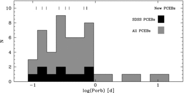
The period distribution of 41 PCEBs from the Ritter & Kolb (2003) (V7.9) catalogue containing a white dwarf plus M or K companion star (grey). The seven systems studied in this paper and the recent PCEB discovery SDSS J143547.87+373338.5 (Steinfadt et al. 2008) are also included. In black is shown a subsample of SDSS PCEBs obtained from RV variation studies. Both subsamples illustrate a clear lack of systems at orbital periods greater than 1 d. The seven new systems from this paper and the two systems in Schreiber et al. (2008) are indicated as tick marks in the top of the figure.

Open in new tabDownload slide

8 CONCLUSIONS

We have presented a study of 11 PCEB previously identified candidates, and measured the orbital periods of six and one of them from their Na i doublet radial velocity variations and its differential photometry, respectively. Combining the K_sec velocity amplitudes with the results from spectroscopic decomposition/fitting of their SDSS spectra, we constrained the binary parameters of the seven systems for which we could determine orbital periods. No radial velocity variations were detected for three PCEB candidates, suggesting that they may be wide binaries. We revisited the PCEB candidate selection of Rebassa-Mansergas et al. (2007), and conclude that candidates with low-amplitude velocity variations, noisy SDSS spectra and radial velocity shifts that only show up in the Hα emission line definitely need additional follow-up spectroscopy for the confirmation/rejection of their PCEB nature. Finally, we have had a first look at the period distribution of PCEBs from SDSS identified from radial velocity snapshots of SDSS WDMS binaries, and noted that none of the 10 systems published so far has an orbital period >1 d. Using a Monte Carlo simulation, we demonstrated that our method of finding PCEBs should be efficient also for systems with periods >1 d, and that, subject to small number statistics, it appears that the PCEB period distribution peaks at P_orb < 1 d. This is in agreement with the period distribution of the previously known PCEBs, which represents a heterogeneous mix of systems identified by various different methods. In contrast, current binary population models predict a large number of PCEBs with orbital periods >1 d in clear disagreement with the currently observed sample. Additional effort is needed to improve the size of the sample of known PCEBs, as well as to fully model its selection effects, but with more than 1000 SDSS WDMS binaries to draw from, the outlook for more quantitative tests of CE evolution seem promising.

AR-M was supported by a STFC-IAC studentship. MRS acknowledges support from FONDECYT (grant 1061199), DIPUV (project 35) and the Centre of Astrophysics in Valparaiso (CAV). ANG-M, AS, RS, JV were supported by the DLR under grant 50OR0404. AS acknowledges support by the DFG grant Schw536/20-1. We thank the referee, John Thorstensen, for providing comments that helped improving the paper.

This paper is based on observations collected at the European Organization for Astronomical Research in the Southern Hemisphere, Chile, under programmes 079.D-0531 and 080.D-0407; at the Centro Astronómico Hispano Alemán at Calar Alto, operated jointly by the Max-Planck-Institut für Astronomie and the Instituto de Astrofísica de Andalucía; at the WHT, which is operated on the island of La Palma by the Isaac Newton Group in the Spanish Observatorio del Roque de los Muchachos of the Instituto de Astrofísica de Canarias; and at the 1.2-m telescope, located at KryoneriKorinthias, and owned by the National Observatory of Athens, Greece. This paper includes data gathered with the 6.5-m Magellan Telescopes located at Las Campanas Observatory, Chile.

REFERENCES