Analytic relations for magnifications and time delays in gravitational lenses with fold and cusp configurations Free

Abstract

1 INTRODUCTION

Gravitational lensing, or the bending of light by gravity, offers an exciting synergy between mathematics and astrophysics. Singularity theory provides a powerful way to describe lensing near critical points (Schneider, Ehlers & Falco 1992; Petters, Levine & Wambsganss 2001), which turns out to have important implications for astrophysics and the quest to understand dark matter. Four-image lensed quasars can be broadly classified, according to image geometry, as folds, cusps or crosses. We are interested in folds and cusps, which occur when the light source is close to the caustic curve, along which the lensing magnification is infinite (see top row of Fig. 1). Fold lenses feature a close pair of bright images, while cusp lenses have a close triplet of bright images (see bottom row of Fig. 1). By expanding the gravitational potential of the lens galaxy in a Taylor series, one finds that the image magnifications satisfy simple analytic relations, viz.

1

for fold pairs and cusp triplets, respectively (Blandford & Narayan 1986; Mao 1992; Schneider & Weiss 1992; Schneider et al. 1992; Gaudi & Petters 2002a,b; Keeton, Gaudi & Petters 2003,2005). For a fold pair, the two images have opposite parity, hence the negative sign. For a cusp triplet, the middle image (B) has opposite parity from the outer images (A and C). Note that in practice, one works with the image fluxes, which are directly observable, rather than the magnifications, which are not. This leads to the equivalent relations:

2

where the image flux F_i is related to the source flux F₀ by F_i= |μ_i|F₀.

Figure 1

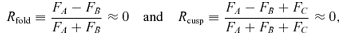
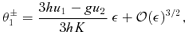
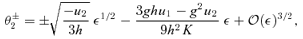
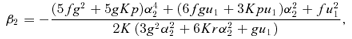
The curves show the caustic (top) and critical curve (bottom) for a SIE lens with minor-to-major axis ratio q= 0.5. The local orthogonal coordinates defined by the rotation matrix are indicated for a fold point (left-hand panel) and a cusp point (right-hand panel). In the top two panels, a source (triangle) with position (y₁, y₂) measured from the centre of the caustic (astroid) has position (u₁, u₂) in the rotated coordinates centred on a fold point (left-hand panel) or a cusp (right-hand panel). In the bottom two panels, the four images (triangles) have positions (x₁, x₂) measured from the centre of the critical curve (ellipse) and positions (θ₁, θ₂) in the rotated coordinates.

Open in new tabDownload slide

Observationally, the fold and cusp relations are violated in several lens systems (e.g. Hogg & Blandford 1994; Falco, Lehar & Shapiro 1997; Keeton, Kochanek & Seljak 1997; Keeton et al. 2003,2005). These so-called ‘flux-ratio anomalies’ are taken as strong evidence that lens galaxies contain significant small-scale structure (e.g. Mao & Schneider 1998; Metcalf & Madau 2001; Chiba 2002). Since global modifications of the lens potential (modelled with multipole terms, for example) cannot explain the anomalous flux ratios (Evans & Witt 2003; Congdon & Keeton 2005; Yoo et al. 2005,2006), it is generally believed that lens galaxies must contain substructure in the form of mass clumps on a scale ≳10⁶M_⊙ (Dobler & Keeton 2006). Indeed, substructure is observed in at least two lens systems, in the form of a dwarf galaxy near the main lens galaxy (Schechter & Moore 1993; McKean et al. 2007). The substructure could well be invisible, though; numerical simulations of structure formation in the cold dark matter (CDM) paradigm predict that galaxy dark matter haloes are filled with hundreds of dark subhaloes (e.g. Klypin et al. 1999; Moore et al. 1999). The abundance of flux-ratio anomalies in lensed radio sources implies that lens galaxies contain ∼2 per cent (0.6–7 per cent at 90 per cent confidence) of their mass in substructure (Dalal & Kochanek 2002). This may be somewhat higher than the amount of CDM substructure (e.g. Mao et al. 2004), although new higher-resolution simulations are attempting to refine the theoretical predictions and make more direct comparisons with lensing observations (e.g. Gao et al. 2004; Diemand, Kuhlen & Madau 2007; Strigari et al. 2007). While there is still work to be done along these lines, it is clear that violations of the ideal fold and cusp relations provide important constraints on the small-scale distribution of matter in distant lens galaxies.

Keeton et al. (2003,2005) pointed out that the ideal fold and cusp relations only hold for a source asymptotically close to the caustic. If we want to use flux-ratio anomalies to study small-scale structure in lens galaxies, it is vital that we understand how much R_fold and R_cusp can deviate from zero for realistic smooth lenses just because the source lies a small but finite distance from the caustic. To that end, Keeton et al. (2003) used a Taylor series approach to demonstrate that R_cusp= 0 to lowest order, and used Monte Carlo simulations to suggest that R_cusp∝d², where d is the distance between the two most widely separated cusp images. In order to derive the leading non-vanishing term in R_cusp analytically, it would be necessary to extend the Taylor series to a higher order of approximation. This has not been done before, since including higher-order terms substantially complicates the analysis. Instead, previous authors have made assumptions about which terms are important and which terms can be neglected, in order to obtain an analytically manageable problem.

As we will see, perturbation theory provides a natural way to overcome the difficulties of the Taylor series approach. Keeton et al. (2005) used perturbation theory to show that for fold lenses, R_fold is proportional to the image separation d₁ of the fold pair. We extend their analysis in several important ways. We derive the leading-order non-vanishing expression for R_cusp using perturbation theory. We also show, for the first time, how the combination of singularity theory and perturbation theory can be used to study time delays between lensed images for both fold and cusp systems. Working in analogy to flux ratios, we derive time-delay relations for fold and cusp lenses, which we will apply (in a forthcoming paper) to observed lenses in order to identify ‘time-delay anomalies’. As time delays join flux ratios in probing small-scale structure in lens galaxies (see Keeton & Moustakas 2008), singularity theory and perturbation theory once again provide the rigorous mathematical foundation.

2 MATHEMATICAL PRELIMINARIES

To study lensing of a source near a caustic, it is convenient to work in coordinates centred at a point on the caustic. Non-spherical lenses typically have two caustics. The ‘radial’ caustic separates regions in the source plane for which one (outside) and two (inside) images are produced. 1 Within the radial caustic is the ‘tangential’ caustic or astroid, which separates regions in the source plane for which two (between the two caustics) and four (inside the astroid) images are produced. We are interested in four-image lenses, where the source is within the astroid. We therefore make no further reference to the radial caustic. A typical astroid is shown in Fig. 1 for a lens galaxy modelled by a singular isothermal ellipsoid (SIE), which is commonly used in the literature (e.g. Kormann, Schneider & Bartelmann 1994) and appears to be quite a good model for real lens galaxies (e.g. Rusin & Kochanek 2005; Koopmans et al. 2006). It is customary to define source-plane coordinates (y₁, y₂) centred on the caustic and aligned with its symmetry axes. However, for fold and cusp configurations, where the source is a small distance from the caustic, it is more natural to work in coordinates (u₁, u₂) centred on the fold or cusp point. For convenience, we define the u₁ axis tangent to (and the u₂ axis orthogonal to) the caustic at that point. Transforming from the (y₁, y₂) plane to the (u₁, u₂) plane requires a translation plus a rotation. To derive this coordinate transformation, we follow the discussion in appendix A1 in Keeton et al. (2005), which summarizes the results of Petters et al. (2001).

We begin by considering the lens equation y=x−∇ψ(x), which maps the image plane to the source plane. The solutions to this equation give the image positions x≡ (x₁, x₂) corresponding to a given source position y≡ (y₁, y₂). The function ψ(x) is the scaled gravitational potential of the lens galaxy projected on to the lens plane. A caustic is a curve along which the magnification is infinite, i.e. ⁠, where ∂y/∂x is the Jacobian of y, and is known as the inverse magnification matrix. We choose coordinates such that the origin of the source plane (y= 0) is on the caustic. In addition, we require that the origin of the lens plane (x= 0) maps to the origin of the source plane. We are interested in sources that lie near the caustic point (y= 0), which give rise to lensed images near the critical point (x= 0). In this case, we may expand the lens potential in a Taylor series about the point x= 0. We then find that the inverse magnification matrix at x= 0 is given by

3

where

4

The subscripts indicate partial derivatives of ψ with respect to x. Note that ψ has no linear part (since y= 0 when x= 0). For y= 0 to be a caustic point, we must have ⁠. In addition, at least one of and must be non-zero (Petters et al. 2001, p. 349). Consequently, and cannot both vanish. Without loss of generality, we assume that ⁠.

We now introduce the orthogonal matrix (see Petters et al. 2001, p. 344)

5

which diagonalizes ∂y/∂x|₀. We then define new orthogonal coordinates by

6

Note that the coordinate changes are the same in the lens and source planes. The advantage of using the same transformation in both the lens and source planes is that the lens equation takes the simple form

7

and that the inverse magnification can be written as

8

The old and new coordinate systems in the source and image planes are shown in Fig. 1. Since the caustic in the source plane maps to the critical curve in the image plane, the origin of the (θ₁, θ₂) frame is determined from that of the (u₁, u₂) frame. The orientation of the (θ₁, θ₂) axes is determined by the matrix ⁠, and is not necessarily related to the tangent to the critical curve.

Using the local orthogonal coordinates u and θ, Petters et al. (2001, p. 346) showed that x= 0 is a fold critical point if and only if the following conditions hold

9

For a cusp, the third condition above is replaced by the requirements that

10

Note in particular that ψ₂₂₂(0) = 0 for a cusp while ψ₂₂₂(0) ≠ 0 for a fold; this indicates that these two cases must be treated separately.

We are interested in obtaining the positions, magnifications and time delays of images near critical points. Since these quantities depend only on the behaviour of the lens potential near a fold or cusp point, we can expand ψ(θ) in a Taylor series about the point θ= 0. To obtain all the quantities of interest to leading order, we must expand the lens potential to fourth order in θ (Petters et al. 2001, pp. 346–347):

11

where the coefficients {K, e, f, g, …, r} are partial derivatives of the potential evaluated at the origin. Lensing observables are independent of a constant term in the potential, so we have not included one. Since θ= 0 maps to u= 0, any linear terms in the potential must vanish. In the second-order terms, the coefficients of the θ₁θ₂ and θ²₂ terms are set to 0 and 1/2, respectively, in order to ensure that the point θ= 0 is a critical point (see appendix A1 of Keeton et al. 2005).

3 THE FOLD CASE

In this section, we use perturbation theory (e.g. Bellman 1966) to derive an analytic relation between the time delays in a fold pair. To derive this expression, we must first obtain the image positions at which the time delay is evaluated. These results were derived by Keeton et al. (2005). We offer a summary of their analysis in Section 3.1 and present our new results for the time delay in Section 3.2.

3.1 Image positions

Since we are considering a source near a fold point, we write its position in terms of a scalar parameter ε, which we take to be small but finite. In particular, let u→εu. Combining equations (7) and (11), we can write the lens equation as

12

13

(see Petters et al. 2001, theorem 9.1). To find the image positions, we expand θ₁ and θ₂ in a power series in ε. Since the left-hand sides of equations (12) and (13) are accurate to ⁠, the right-hand sides must be accurate to the same order. Noting that the lowest-order terms on the right-hand side are linear or quadratic in θ, we write

14

15

Substituting into the lens equation, we obtain

16

17

Note that these equations are carried to different orders in ε, since the leading-order term in equation (12) is linear in θ, while the leading-order term in equation (13) is quadratic in θ.

Since ε is non-zero, equations (16) and (17) must be satisfied at each order in ε. We can work term by term to solve for the coefficients α₁, α₂ and β₂, and then write the image positions as

18

19

where the ± labels indicate the parities of the images. From these equations, we see that two images form near the point θ= 0 on the critical curve, provided that (−u₂/3h) > 0. Since h≤ 0 for standard lens potentials (e.g. an isothermal ellipsoid or isothermal sphere with shear), we must have u₂ > 0. In other words, the source must lie inside the caustic in order to produce a pair of fold images. In practice, a more useful quantity is the image separation, given by

20

3.2 Time delays

To find the time delay between the two fold images, we begin with the general expression for the scaled time delay (e.g. Schneider et al. 1992):

21

The scale factor is given by

22

where D_L, D_S and D_LS are the angular-diameter distances from the observer to lens, observer to source and lens to source, respectively. The lens redshift is denoted by z_L. Making the substitution u→ (εu₁, εu₂), we have for the two fold images

23

24

The time delay between images is then (c.f. Schneider et al. 1992, pp. 190–191)

25

which is positive, in agreement with the general result that images with negative parity trail those with positive parity. We find that the only coefficient from the lens potential that enters the expression for the differential time delay is the parameter h=ψ₂₂₂(0)/6. We also see that to leading order in ε, the image separation and the differential time delay depend only on the u₂ component of the source position. Unlike the image positions, our expression for the time delay does not involve any of the fourth-order terms in the potential. This is because the time delay involves the potential directly, while the image positions depend on first derivatives of the potential. This means that all fourth-order terms in the potential enter the time delay at ⁠, while these same terms enter at in quantities involving derivatives.

To summarize, ⁠. For comparison, R_fold∝d₁. Since d₁ is small, a violation of the ideal relation is more likely to indicate the presence of small-scale structure in the lens galaxy than would be indicated by a non-zero value of R_fold.

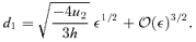
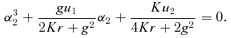
Our analytic expression for is only valid for sources sufficiently close to the caustic that higher-order terms are negligible. To quantify this statement, we compare our analytic approximation with the differential time delay computed numerically from the exact form of the lens equation. The numerical analysis requires a specific lens model, so we consider a SIE with axis ratio q= 0.5 as a representative example. We use the software of Keeton (2001) to compute the astroid caustic, and then choose a point on the caustic, far from a cusp, to serve as the origin of the (u₁, u₂) frame. For a given value of u₂, we solve the exact lens equation to obtain the image positions and time delay for the fold doublet. The top left panel of Fig. 2 shows in units of θ²_E as a function of u₂ in units of θ_E, where θ_E is the Einstein angle of the lens. The analytic and numerical results are in good agreement for sources within 0.05θ_E of the caustic, although the curves do begin to diverge as u₂ increases. The difference between the numerical and analytic curves (which represents the error in the analytic approximation, denoted by ɛ) is shown in the middle left panel. The bottom left panel shows the logarithmic slope of the error curve, d(ln ɛ)/d(ln u₂). Together, the middle and the bottom left panels verify that our analytic approximation is accurate at the order of ε^3/2. Furthermore, these panels suggest that the next non-vanishing term is of the order of ε^5/2 and has a positive coefficient. The interesting implication is that the coefficient of the ε² term seems to vanish. At our current order of approximation, we are not able to determine whether this is rigorously true, and if so, how general it is; we merely offer the remark in the hope that it may be useful for future analytic studies. For now, we focus on the verification that our analytic approximation is accurate at the order to which we work.

Figure 2

The top panels show the time delay for a fold pair as a function of source position (left-hand panel) and image separation (right-hand panel), for a SIE lens with axis ratio q= 0.5. The solid line shows our analytic approximation while the dotted line shows the exact result obtained by solving the lens equation numerically. The quantities u₂ and d₁ are defined in the text, and are shown here in units of the Einstein angle, θ_E. The time delay is given in units of θ²_E. The middle panels show the error in the analytic approximation, ⁠, due to our neglect of higher-order terms. The bottom panels show the logarithmic slope of the error curve, d(ln ɛ)/d(ln u₂) on the left-hand side and d(ln ɛ)/d(ln d₁) on the right-hand side. There is some numerical noise in the logarithmic slope due to numerical differentiation. Together, the middle and bottom panels verify that our analytic expression is accurate at order ε^3/2 (cf. equation 25).

Open in new tabDownload slide

Since the source position u₂ is not observable, we compare the analytic and numerical time delays as a function of the image separation d₁ in the right-hand panels of Fig. 2. The range of d₁ corresponds to that used for u₂ in the left-hand panels. For a canonical fold lens with d₁= 0.46θ_E (Keeton et al. 2005), our analytic expression gives a very good approximation, indicating that our analysis can be applied in astrophysically relevant situations – not just when the source is asymptotically close to the caustic, but even when it lies some small but finite distance away.

4 THE CUSP CASE

We now apply our perturbative method to the case of a source near a cusp point. This approach has not been applied to cusp lenses before. Appendix A of Keeton et al. (2003) derives the image positions and magnifications for a cusp triplet assuming a simplified form of the lens equation. As we noted in Section 1, this simplified lens equation assumes that certain terms may be set to zero, using criteria that are less than rigorous. We use the lens equation derived from the fourth-order lens potential, and use perturbation theory to verify the results of Keeton et al. (2003) and extend the analysis to a higher order of approximation. We also study time delays for a cusp lens for the first time. Our analysis does not involve simplifying assumptions, and indicates that perturbation theory is a powerful method in the study of lensing.

4.1 Image positions

We again expand the image positions, magnifications and time delays in the parameter ε, but with one notable difference. For a cusp oriented in the u₁ direction, a small ‘horizontal’ displacement of εu₁ from the cusp point permits a ‘vertical’ displacement of only ε^3/2u₂ (see Fig. 1), since larger vertical displacements would imply a source position outside the caustic (Blandford & Narayan 1986). The lens equation is then

26

27

(see Petters et al. 2001, theorem 9.1), where the θ²₂ term of equation (13) does not appear, since ψ₂₂₂(0) = 0 for a cusp, corresponding to h= 0 in equation (11).

As before, we write the image positions as a series expansion in ε, but now keeping an additional term (i.e. γ_iε^3/2). This is necessary since the vertical component of the source position enters the lens equation as ε^3/2u₂, rather than εu₂, as in the fold case. We have

28

29

The lens equation then becomes

30

31

As in the fold case (see equation 16), we find α₁= 0. Note that γ₂ appears only in the ε² coefficient of equation (31), but in a term multiplied by α₁. Hence, it will not be possible to solve for γ₂. Fortunately, it turns out that the expressions we would like to derive do not involve this parameter.

We can now write the lens equation as

32

33

Recalling that these equations must be satisfied at each order in ε, we then solve for the unknown coefficients:

34

35

36

where α₂ satisfies the cubic equation

37

This is equivalent to equation (A8) from Keeton et al. (2003), after making the replacements α₂→z, K→c, g→−b/2, r→−a/4. To leading order, the image positions can be written as

38

39

which are equivalent to equation (A7) from Keeton et al. (2003). The distance between any two images i and j is then

40

4.2 Magnifications

Substituting our perturbative expressions for the image positions into equation (8), we find that the inverse magnification of a cusp image is given by

41

We then find from equation (2) that

42

where d= max_ijd_ij is the largest separation between any two of the three cusp images. This expression shows that correction terms to the ideal cusp relation enter at second order in the image separation, which agrees with the conjecture of Keeton et al. (2003). To see this, we define m_i≡ |μ⁻¹_i|, which allows us to write

43

If the leading-order term in the numerator vanishes, so does the leading-order term in R_cusp. The zeroth-order term in R_cusp corresponds to a term of in the numerator, since the leading-order term in the denominator is ⁠. By substituting the solutions for α₂ into the numerator, we find that R_cusp= 0 to lowest order, in agreement with Keeton et al. (2003). We repeat this procedure for the next-leading term of in the numerator, and find that R_cusp= 0 at linear order in d[i.e. 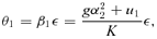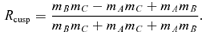] as well; this result was unattainable using the formalism of Keeton et al. (2003). To proceed to higher order, we must extend our perturbative analysis by including terms of the form δ_iε² in equations (28) and (29) for the image positions. We denote the coefficient of d² by A_cusp, which we do not write down here, since that would require several pages. Given the complexity of this term, it is not practical to evaluate A_cusp analytically. However, we have numerically computed R_cusp for the case of a SIE model with q= 0.5 (see Fig. 3) and find that R_cusp∝u₁∝d². While it is conceivable that A_cusp might be zero for some specific lens model, this is clearly not the case in general. We have thus analytically demonstrated that R_cusp vanishes through linear order in d, placing the numerical result of Keeton et al. (2003) on solid mathematical ground.

Figure 3

R_cusp as a function of u₁ (left-hand panel) and d (right-hand panel) for a SIE with q= 0.5, obtained by solving the lens equation numerically.

Open in new tabDownload slide

4.3 Time delays

For the cusp case, the scaled time delay takes the form

44

We find

45

corresponding to a differential time delay of

46

Unlike the fold case, the time delay for a pair of cusp images depends on both source coordinates (u₁, u₂). This means that it is not possible to write our current expression strictly in terms of observables, such as the image separation. Instead, all we can say is that the time delay scales quadratically with ε, or alternatively, with the fourth power of the image separation.

In the fold case, we found that the time delay scales as ε^3/2 and only depends on the lens potential through the parameter h. For a cusp, however, h= 0, so it is not surprising that the lowest-order term in the time delay is of ⁠. Furthermore, if we had not included the γ_i ε^3/2 terms in our expansions of the image positions for a cusp (equations 28 and 29), it would not have been possible to obtain a perturbative expression for the time delay; instead, we would simply have found ⁠.

5 SUMMARY

We have developed a unified, rigorous framework for studying lensing near fold and cusp critical points, which can (in principle) be extended to arbitrary order. We have found that the differential time delay of a fold pair assumes a particularly simple form, depending only on the image separation and the Taylor coefficient h=ψ₂₂₂(0)/6. This result is astrophysically relevant, since it is quite accurate even for sources that are not asymptotically close to the caustic. We have also obtained perturbative expressions for the image positions, magnifications and time delays of a cusp triplet. These results rest on the key insight that a source at a given distance ε from a cusp along the relevant symmetry axis of the caustic can only move a perpendicular distance of ε^3/2 in order to remain inside the caustic (Blandford & Narayan 1986). We have shown rigorously that the distance dependence of the magnification ratio R_cusp conjectured by Keeton et al. (2003) is correct. We have also demonstrated that the leading-order expression for the image positions is given by the relations presented by Keeton et al. (2003), and have provided the necessary framework for deriving the image positions corresponding to a Taylor expansion of the lens potential at arbitrary truncation order. Finally, we have derived cusp time delays analytically for the first time. Our results provide a rigorous foundation for identifying anomalous flux ratios and time delays in gravitational lens systems, and for using them to study small-scale structure in the mass distributions of distant galaxies.

We thank A. O. Petters and Peter Schneider for helpful discussions and suggestions, and for their careful reading of the manuscript. We also thank the anonymous referee for useful comments.

REFERENCES