Broad reprocessed Balmer emission from warped accretion discs Free

Abstract

1 INTRODUCTION

A small fraction of active galactic nuclei (AGN) show double-peaked broad emission-line profiles (Eracleous & Halpern 1994; Eracleous & Halpern 2003; Strateva et al. 2003; Gezari, Halpern & Eracleous 2007). The possibility has been considered for a long time that at least some of these lines arise directly from the accretion discs assumed to feed the central supermassive black holes. The Hα profile observed in the spectrum of Arp 102B was modelled as arising in a relativistic disc by Chen & Halpern (1989) and Chen, Halpern & Filippenko (1989) in an attempt to explain the asymmetric double-peaked profiles. In these stationary circular relativistic disc models, Doppler boosting will make the blue peak of the profile higher than the red one. However, Miller & Peterson (1990) questioned the relativistic disc explanation for Arp 102B, by showing that at least at some epochs the profile asymmetry is reversed, with the red peak higher than the blue one in contrary to the prediction of homogeneous, circular relativistic disc models. This type of profile asymmetry has been observed in some other double-peaked sources (Strateva et al. 2003; Gezari et al. 2007). Thus, other scenarios for the profile asymmetry were considered later on, including various physically plausible processes in the accretion flow, such as spiral shocks, eccentric discs, bipolar outflows (Zheng, Sulentic & Binette 1990; Veilleux & Zheng 1991; Chakrabarti & Wiita 1993,1994; Eracleous et al. 1995; Storchi-Bergmann et al. 1997), as well as a binary black hole system (Begelman, Blandford & Rees 1980; Gaskell 1996; Zhang, Dultzin-Hacyan & Wang 2007b).

In addition to the line profile asymmetry, the energetic budget for the line emission region has not been solved so far for the disc model. It is demonstrated that the local viscous heating in the accretion disc is not sufficient to explain the observed Hα intensity (Chen et al. 1989; Eracleous et al. 1997), thus reprocessing of ultraviolet (UV)/X-ray continuum from the inner accretion disc is required. However, only a very small fraction of radiation from inner disc is expected to intercept the outer part of the disc in the case of a flat geometrically thin disc. Two types of processes have been proposed to increase the fraction of light incident on to the disc emission-line region. Chen et al. (1989) proposed that the inner part of the accretion disc is hot and becomes geometrically thick due to insufficient radiative cooling, and the X-ray emission from such an ion-supported torus is responsible for such energy input. However, double peak emitters do not always have a low accretion rate (Bian et al. 2007; Zhang, Dultzin-Hacyan & Wang 2007a). Furthermore, a detailed calculation of advection-dominated accretion flow (ADAF) models suggests that only a small portion of X-rays actually hit the emission-line portion of the disc (Cao & Wang 2006). On the other hand, Cao & Wang (2006) proposed that a slow-moving jet can scatter a substantial fraction of UV/X-ray light from the inner accretion disc back to the outer part of the disc. While this may be the likely case for radio-loud double-peaked emitters, the majority of double-peaked emitters are radio-quiet.

On the other hand, warped accretion discs are believed to exist in a variety of astrophysical systems, including X-ray binaries, T Tauri stars and AGN. The dynamics of warping accretion discs has been discussed by a number of authors (Papaloizou & Pringle 1983; Papaloizou & Lin 1995; Nelson & Papaloizou 1999; Ogilvie 1999; Nelson & Papaloizou 2000; Nayakshin 2005). Four main mechanisms for exciting/maintaining warping in accretion discs have been proposed, including: tidally induced warping by a companion in a binary system (Terquem & Bertout 1993; Larwood et al. 1996; Terquem & Bertout 1996), radiation driven or self-inducing warping (Maloney, Begelman & Pringle 1996; Pringle 1996; Maloney & Begelman 1997; Pringle 1997; Maloney, Begelman & Nowak 1998), magnetically driven disc warping (Lai 1999,2003; Pfeiffer & Lai 2004), and frame dragging driven warping (Bardeen & Petterson 1975; Kumar & Pringle 1985; Armitage & Natarajan 1999). As a result, the accretion disc in some AGN should be non-planar. Evidence for the existence of warped discs in AGN has been found by observations (Herrnstein et al. 2005; Caproni et al. 2007). A warped disc makes it possible for the radiation from the inner disc to reach the outer parts, enhancing the reprocessing emission lines. Thus, this warping can solve the long-standing energy-budget problem because the subtending angle of the outer disc portion to the inner part has been increased by the warp. It can also provide the asymmetry required for the variations of the emission lines. The effect of disc warping on iron line profiles treated relativistically have been made by Hartnoll & Blackman (2000) and Čadež et al. (2003). Bachev (1999) studied the broad-line Hβ profiles from a warped disc. Nevertheless, his treatment is non-relativistic. A relativistic treatment of warped disc on the Balmer lines which can be compared with observations is still not available in the literature.

In this paper, the broad Balmer emission due to reprocessing of the central high-energy radiation by a warped accretion disc is investigated. Our main purpose here is to describe the effect of disc warping on the line profiles. A parametrized disc model is adopted. In Section 2 we summarize the assumptions behind our model, and present the basic equations relevant to our problem. We present our results and the comparison with observations in Section 3, and conclusion and discussion in Section 4.

2 ASSUMPTIONS AND METHOD OF CALCULATION

In this paper, we will focus on how a warped disc affects the optical emission-line profiles, such as Hα and Hβ. A geometrically thin disc and a central point-like source of ionizing radiation around a black hole are assumed.

2.1 Geometrical considerations

The disc can be treated as being composed of a series of concentric circular rings of increasing radii, and laying in different planes. The rings interact with each other via viscous stresses. Each ring is defined by two Eulerian angles β(R, t) and γ(R, t) (see Fig. 1) at radius R, where β(R, t) is the tilt angle of the disc with respect to the normal to the equatorial plane, while the twist angle γ(R, t) describes the orientation of the line of nodes with respect to a fixed axis in the equatorial plane. Note that R is a purely radial coordinate and not the cylindrical one. At each radius R from the centre, the disc has a unit tilt vector l(R, t) which varies continuously with radius R and time t. Following Pringle (1996), in an inertial frame OXYZ centred on the disc, the vector l(R, t) is given by

1

We define the normalized vector towards the observer as

2

where i is the angle between the line of sight and the normal to the equatorial plane lie in the XZ plane.

Figure 1

The geometry used in this paper. The warped accretion disc is modelled as a collection of inclined rings, each defined by two Eulerian angles β, γ and the radial distance R. The normal to the equatorial plane is aligned with the Z direction. The direction to the observer is denoted by i that is the angle between the direction of line of sight and the Z-axis.

Open in new tabDownload slide

We define the coordinates on the surface of the disc as (R, φ) with respect to a fixed Cartesian coordinate system (x, y, z), where φ is the azimuthal angle measured on the disc surface in the direction of flow, with φ=π/2 at the ascending node.1 The position vector of a point on the ring of radius R is R=Re_R, where

3

is the radial unit vector. Note that l·e_R= 0, since points on the ring lie in the plane that passes through the origin and is orthogonal to l. Now (R, φ) are (in general) non-orthogonal coordinates on the surface of the disc. The element of surface area is

4

by calculating these partial derivatives directly and after some algebra which simplifies to

5

where the primes indicate differentiation with respect to R, and hence, since l·e_R= 0,

6

The radiation flux L received from the central parts by the unit area is proportional to

7

if the element in question is not obscured by other interior parts of the disc, otherwise the flux is set to zero (see below). The Balmer lines in the illuminated surface are formed as a result of photoionization by UV/X-ray radiation from inner accretion disc. We assume that Balmer line intensity is proportional to the radiation being intercepted by the disc, thus the line emissivity ɛ on the disc surface can take the form ɛ∝L. A detailed treatment of line emission requires solving the vertical structure as well as the radiative transfer in the disc explicitly, which is beyond the scope of this paper. We also assume that the line emission is isotropic in the comoving frame.

An alternative useful formalism being used to describe the shape of the warped disc is introducing the scaleheight of the disc which is the displacement in the direction normal to the equatorial plane. The scaleheight denoted by h(r, ϕ) is a function of radius r and azimuthal angle ϕ in cylindrical coordinates with respect to Cartesian coordinate system (X, Y, Z). The two formalisms described above can be related by the formula

8

where ψ=ϕ−γ and it satisfies

9

Since it is difficult to calculate analytically the disc distortion induced by combined action of external torques mentioned above, here we do not consider the disc dynamics, and merely parametrize the disc geometry to capture the main characteristics of emission-line profiles from warped discs. In this paper, a steady disc is adopted, and the form of the two angles γ, β as a function of radius R are given by

10

11

where R_in and R_out are the disc inner and outer radii, n_i (i= 1, 2, 3) are three free parameters used to describe the warped disc geometry, γ₀ is a constant which is used to describe the longitude of the observer with respect to the coordinate system of the disc. This angle is mathematically equivalent to changing observational time for possible precession. Thus, the line profiles with different γ₀ can be compared with the data observed at different times.

2.2 Photon motions in the background metric

The propagation of radiation from the disc around a Kerr black hole and the particle kinematics in the disc were studied by many authors (Carter 1968; Bardeen, Press & Teukolsky 1972). We review properties of the Kerr metric and formulae for its particle orbits, and summarize here the basic equations relevant to this paper. Throughout the paper we use units in which G=c= 1, where G is the gravitational constant, c is the speed of light. In Boyer–Lindquist coordinates, the Kerr metric is given by

12

where

Here M, a are the black hole mass and specific angular momentum, respectively.

The general orbits of photons in the Kerr geometry can be expressed by a set of three constants of motion (Carter 1968). Those are the energy at infinity E, the axial component of angular momentum Eλ and Carter's constant ⁠. The 4-momentum of a geodesic has components

13

with

From this, the equations of motion governing the orbital trajectory can be obtained. The motion in the r–θ plane is governed by (Bardeen et al. 1972)

14

where r_e and θ_e are the starting values of r and θ. The φ coordinate along the trajectory is calculated by (Wilkins 1972; Viergutz 1993)

15

Consider the orbit equation in the form

16

where r_ms is the radius of the marginally stable orbit for a maximal Kerr black hole, a= 0.998. Then θ can be expressed in terms of P as follows (Čadež, Fanton & Calvani 1998):

17

where m=μ²₊/(μ²₊+μ²₋), μ²_± are defined by

18

and

19

where K(m) is the complete elliptic integral of the first kind.

For photons emitted from radii (>100r_g) propagating to infinity the differences between Kerr and Schwarzschild black holes are indistinguishable. Neglecting terms of order 1/r² and higher, the Kerr metric reduces to the Schwarzschild metric. The formulae for the particle orbits in this case are simplified. Here we summarize the basic equations relevant to this paper. The line element in Schwarzschild geometry is written as follows:

20

The observer is assumed to be located at (r_o, ϑ_o, φ_o). For an approximately spherical background, each inclined ring of the disc can be considered lying in the equatorial plane. Owing to a spherically symmetric metric there is no favoured direction for the black hole; in this sense, ϑ_o can be acted as the angle between the observer and the normal to the disc and is determined by taking the dot products of the unit vector l of the disc with the normalized vector i_obs to the observer. By definition, we get

21

The angle φ₀ can be obtained by setting the mixed triple product of three vectors i_obs, l and e_R equal zero, (i_obsle_R) = 0. From this equation, the angle is determined by

22

The photon motion equations are given by (Lu & Yu 2001)

23

24

where r_e, ϑ_e and φ_e are the starting values of r, ϑ and φ.

Define μ= cos ϑ, then in equations (23) and (24) the integral over μ can be worked out in terms of a trigonometric integral

25

26

where 0 ≤μ < μ₊, and Θ_μ(μ) =q²− (λ²+q²)μ². The integral over r can be worked out with inverse Jacobian elliptic integrals (see e.g. Čadež et al. 1998; Wu & Wang 2007).

Although our calculation is limited to Schwarzschild metric for photons travelling to infinity, for the radii (>100 r_g) taken into account in this paper, the results are essentially the same for the Kerr black hole. On the other hand, for the light from inner part of the disc, a maximal Kerr metric is still used.

2.3 The observed line flux

Due to relativistic effects, the photon frequency will shift from the emitted frequency ν_e to the observed one ν_o received by a rest observer with the hole at infinity. We introduce a g factor to describe the shift which is the ratio of observed frequency to emitted one:

27

where Ω=r^−3/2 is the Keplerian angular velocity, p, u_o, u_e are the 4-momentum of the photon, the 4-velocity of the observer and the emitter, respectively.

The specific flux density F_o(ν_o) at frequency ν_o as observed by an observer at infinity is defined as the sum of the observed specific intensities I_o(ν_o) from all parts of the accretion disc surface, which is given by (Cunningham 1975)

28

where dΩ_obs is the element of the solid angle subtended by the image of the disc on the observer's sky and we have made use of the relativistic invariance of I_ν/ν³, ν is the photon frequency measured by any local observer on the path. I_e(ν_e) is the specific intensity measured by an observer corotating with the disc, and can be approximated by a δ function, I′_e(ν′_e) =ɛδ(ν′_e−ν_e), where ɛ is the emissivity per unit surface area. From well-known transformation properties of δ functions we have δ(ν′_e−ν_e) =gδ(ν_o−gν_e); using this in equation (28), we obtain

29

In order to calculate the integration over d Ω_obs, using two impact parameters α and β, measured relative to the direction to the centre of the black hole, first introduced by Cunningham & Bardeen (1973) is convenient. They are related to two constants of motion λ and q by equations

30

The element of solid angle seen by the observer is then

31

where r_o is the distance from the observer to the black hole.

Substituting equation (31) into equation (29) gives the desired result:

32

In the calculation of the total flux of reprocessing emission line, shadowing of the elements by the inner parts of the disc must be taken into account. This has been done as follows. The contribution of each element denoted by (r, ϕ) to the total line flux from the disc is calculated by equation (32) only in the case that there does not exist another element with cos θ_i > cos θ(r_i, ϕ_i) tracing the trajectory of photon, and is zero in the opposite case. Here cos θ_i=h(r_i < r, ϕ_i)/r_i, ϕ_i and cos θ(r_i, ϕ_i) are calculated by equations (15) and (17), respectively:

33

34

Equation (33) is obtained by setting λ= 0 in equation (15) as an approximation for a point-like source assumption. In the calculation, the disc is divided into 1000 rings logarithmically spaced in radial direction, and we checked every increment of r for the inequality along the ray path. In the calculation we neglect the contribution from the lower surface of the disc or the higher order images of the emitter due to the fact that at low observer inclination angles the extra flux is small compared to the direct images. And a more correct calculation will need to handle these effects correctly and may give up to a factor of 2 change in the central region (see e.g. Viergutz 1993).

2.4 Method of calculation

With all of the preparation described in the previous section, we now turn to how to calculate the line profiles numerically. We divide the disc into a number of arbitrarily narrow rings, and emission from each ring is calculated by considering its axisymmetry. We shall denote by r_i the radius of each such emitting ring. For each ring there is a family of null geodesics along which radiation flows to a distant observer at polar angle ϑ_o from the disc's axis. As far as a specific emission line is concerned, for a given observed frequency ν_o the null geodesics in this family can be picked out if they exist. So, the weighted contribution of this ring to the line flux can be determined. The total observed flux can be obtained by summing over all emitting rings.

The main numerical procedures for computing the line profiles are as follows.

• Specify the relevant disc system parameters: r_in, r_out, n₁, n₂, n₃ and i, γ₀.

• The flux from the disc surface is integrated using Gauss–Legendre integration with an algorithm due to G. B. Rybicki (Press et al. 1992). The routine provides abscissas r_i and weights ω_i for the integration.

• For a given couple (r_i, g) of a ring, the two constants of motion λ and q are determined if they exist. This is done in the following way. The value of λ is obtained by an alternate form of equation (27):

  

  35

  the value of q is determined for solving photon trajectory equation (23). Then the contribution of this ring on the flux for a given frequency ν_o with respect to g is estimated. Varying g, this step is repeated, thus the flux contribution of this ring to all the possible frequency is obtained.
• For each g, the integration over r of equation (32) can be replaced by a sum over all the emitting rings weighted by ω_i:

  

  36

  The Jacobian [∂(λ, q)/∂(r, g)] in the above formula was evaluated by a finite difference scheme. In the calculation the self-obscuration along the line of sight are also taken into account. This has been done as follows. The contribution of each element denoted by (r_i, g) to the total line flux from the disc is calculated by equation (36) only in the case that there does not exist another element with cos θ_i > cos θ(r_i, ϕ_i) along the ray path, and is zero in the opposite case. Here cos θ_i=h(r_i, ϕ_i)/r_i, cos θ(r_i, ϕ_i) is calculated by

  

  37

  where the first equation describes the case with one turning point in θ component along the geodesic, ϕ_i can be calculated by equations (24) and (26) and P, KM, μ₊ satisfy

  

From the above formula, one determines the line flux at an arbitrary frequency ν_o from the disc. The observed line profile as a function of frequency ν_o is finally obtained in this way.

3 RESULTS

In the accretion disc model, the double-peaked emission lines are radiated from the disc region between around several hundred gravitational radii to more than 2000r_g; here r_g is the gravitational radius and the widths of double-peaked lines range from several thousand to nearly 40 000 km s⁻¹ (Wang et al. 2005). In our model, all of the parameters of the warped disc are set to be free. The reasonable ranges are: disc radius from 100r_g to 2000r_g, n₁ from 0 to 3π, n₂ from 2 to 4, n₂ from 0° to 30°. This model has the same number of free parameters as an eccentric disc model (Eracleous et al. 1995). In the range of frequency from 4.32 to 4.78 in units of 10¹⁴ Hz, 180 bins are used. Considering the broadening due to electron scattering or turbulence, all our results are smoothed by convolution with 3σ Gaussian (corresponding to 500 km s⁻¹).

3.1 Line profiles from twisted warping discs

We extend the numerical code developed by Wu & Wang (2007) to deal with the warped discs. The images of the illuminated area and the Hα line profiles computed by our code for a steady-state twisted warping disc are shown in Figs 2 and 3. The disc zone is from R_in= 100r_g to R_out= 1000r_g, the other parameters are i= 30°, n₁= 2.1π, n₂= 3.0, n₃= 10°, and i= 15°, n₁= 2.1π, n₂= 3.0, n₃= 20°, respectively. The longitude of the observer γ₀ with respect to the coordinate system of the disc from top left-hand side to bottom right-hand side varies from 0° to 330° with a step of 30°. The image of the illuminated portion of the disc has a shape similar to a one-armed disc. The image area of the disc being projected on the observer's sky from the far side of the disc due to a little angle between the tilt vector l(R, t) and the line of sight significantly larger than the near parts are indicated in Figs 2 and 3. In our code, one can specify an arbitrary grid for r or φ. In our calculations, all the images contain 400 × 360 pixels in this paper. The line profiles drawn in black are restricted to prograde disc models (relative to the normal to equatorial plane or black hole spin), the effects of a retrograde disc (identical to the prograde case with a reversed spin) on the line profiles should also be taken into account if the orientations of the AGN are isotropically distributed in space; those are drawn with dotted lines in the plots. The profiles from a prograde disc and its corresponding retrograde disc is close to but not exactly reflective symmetric about v= 0 because of relativistic boosting, the gravitational redshift and the asymmetry of the disc. Note also that there are triple-peaked profiles similar to those found by observations (Veilleux & Zheng 1991) and the obvious variation in the red/blue peak positions.

Figure 2

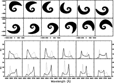
The images (upper panel) of the illuminated area of the disc and Hα line profiles (lower panel) computed by our code for twist warped disc case for i= 30°, n₁= 2.1π, n₂= 3.0, n₃= 10°, the disc zone is from R_in= 100r_g to R_out= 1000r_g. The profiles from both prograde disc (black line) and retrograde disc (dotted line) are shown. The longitude of the observer γ₀ with respect to the coordinate system of the disc takes steps of 30° from 0° to 330° (from top left-hand side to bottom right-hand side). All the results are smoothed by convolution with 3σ Gaussian (corresponding to 500 km s⁻¹).

Open in new tabDownload slide

Figure 3

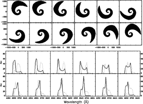
As in Fig. 2 but with i= 15°, n₃= 20°.

Open in new tabDownload slide

The influence of the phase amplitude (described by parameter n₁) on the line profiles for n₁= 0 (twist-free), π, 2π, 3π are shown in Fig. 4. The disc zone is from R_in= 100r_g to R_out= 1200 r_g, the other parameters are i= 30°, n₂= 3.0, n₃= 10°. The longitude of the observer γ₀ with respect to the coordinate system of the disc varies from 0° to 300° with a step of 60° (from left- to right-hand side). For twist-free and low phase amplitude discs, the asymmetric as well as frequency-shifted single-peaked line profiles expected in most cases are produced. For n₁ > 2π, there is a fairly large possibility for a triple-peaked line profile. The influence of the phase amplitude on the line profiles is remarkable.

Figure 4

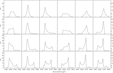
Comparison of the Hα line profiles generated by our code for warped disc cases with different phase amplitude (described by parameter n₁), n₁= 0, π, 2π, 3π (from top to bottom panels). The other parameters are: i= 30°, n₂= 3.0, n₃= 10°, R_in= 100r_g and R_out= 1200r_g. The longitude of the observer γ₀ with respect to the coordinate system of the disc varies from 0° to 300° with a step of 60° (from left- to right-hand side).

Open in new tabDownload slide

The fraction of light incident to the disc from the inner region is a function of n₁, n₃. We calculate the fraction received by a warped disc, the results are shown in Fig. 5. The fraction reaches 27.3 per cent for a twisted warp disc n₁= 2.0π, n₂= 3.0, n₃= 20°.

Figure 5

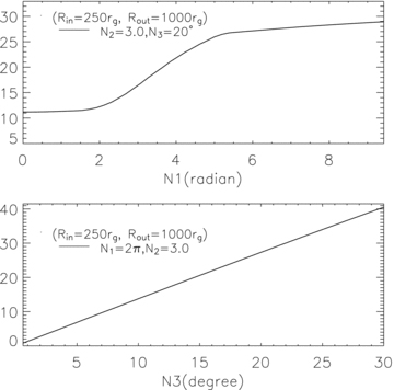
The fraction of light incident to the disc from the inner region as a function of n₁ or n₃. The disc zone is from R_in= 250r_g to R_out= 1000r_g.

Open in new tabDownload slide

3.2 Comparison with the observations

As the first step, our main purpose in this paper is to demonstrate the effect of disc warping on the line profiles, while the detailed fitting of the observational data will be presented in a future paper. From the sample of AGN with double-peaked Balmer lines drawn from the Sloan Digital Sky Survey (SDSS) spectroscopic data set (Shan et al., in preparation), we pick up four sources with peculiar profiles: SDSS J084205.57+075925.5, SDSS J232721.96+152437.3, SDSS J094321.97+042412.0, SDSS J093653.84+533126.8. Two of them have explicit triple-peaked profiles, the others show a net shift of the emission lines to the red. These features are hard to interpret via a homogeneous, circular relativistic disc model. The SDSS spectrum of one object (SDSS J232721.96+152437.3) is dominated by starlight from the host galaxy; we subtract the starlight and the nuclear continuum with the method as described in detail in Zhou et al. (2006). The other three spectra have little starlight contamination, the nuclear continuum and the Fe ii emission multiplets are modelled as described in detail in Dong et al. (2008). The Fe ii emission lines are apparent in J0936+5331.

The observed broad line spectrum of sources SDSS J084205.57+075925.5, SDSS J232721.96+152437.3 both have a third peak. The line profiles (grey line) calculated by our code compared with observations are shown in Figs 6 and 7. The disc zone is from R_in= 250r_g to R_out= 1000 r_g, and n₂= 3.0 for a prograde disc case. The other parameters are: i= 13°, n₁= 3.0π, n₃= 28°, γ₀= 95° for SDSS J084205.57+075925.5, i= 10°, n₁= 2.6π, n₃= 22°, γ₀= 88° for SDSS J232721.96+152437.3, respectively. We have taken the approach that the disc-like component should be fitted by eye to as much of the peaks' match as possible. While our model does not reproduce the extended wing, the peak positions and heights are reasonably in agreement with the observed profiles.

Figure 6

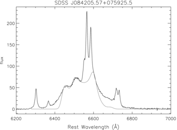
Comparison of the Hα line profiles computed by our code (grey line) with the observation of SDSS J084205.57+075925.5. The parameters are: i= 13°, n₁= 3.0π, n₂= 3.0, n₃= 28°, γ₀= 95°, the disc zone is from R_in= 250r_g to R_out= 1000r_g for a prograde disc.

Open in new tabDownload slide

Figure 7

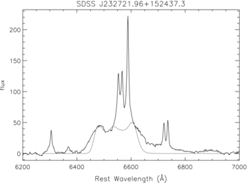
Comparison of the Hα line profiles computed by our code (grey line) with the observation of SDSS J232721.96+152437.3. The parameters are: i= 10°, n₁= 2.6π, n₂= 3.0, n₃= 22°, γ₀= 88°, the disc zone is from R_in= 250r_g to R_out= 1000 r_g for a prograde disc.

Open in new tabDownload slide

A retrograde disc is needed to match the line profiles with the observations for SDSS J094321.97+042412.0, J093653.84+533126.8. Fig. 8 shows the comparison between the line profiles and the observed profile for SDSS J094321.97+042412.0 with i= 17°, n₁= 2.1π, n₃= 24°, γ₀= 202°. And the parameters in Fig. 9 for SDSS J093653.84+533126.8 are: i= 8°, n₁= 2.1π, n₃= 6°, γ₀= 117°. The disc zone is still taken from R_in= 250r_g to R_out= 1000 r_g, and n₂= 3.0. We see that the overall match except that in two wings between the line profiles and the observations is good qualitatively. The deviation in the two wings may, mostly due to the central point-like source adopted, diminish the contribution from the relatively inner part of the reprocessing region.

Figure 8

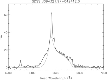
Comparison of the Hα line profiles computed by our code (grey line) with the observation of SDSS J094321.97+042412.0. The parameters are: i= 17°, n₁= 2.1π, n₂= 3.0, n₃= 24°, γ₀= 202°, the disc zone is from R_in= 250r_g to R_out= 1000r_g for a retrograde disc.

Open in new tabDownload slide

Figure 9

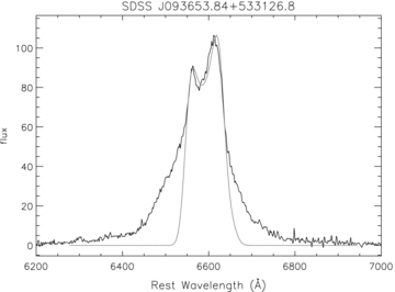
Comparison of the Hα line profiles computed by our code (grey line) with the observation of SDSS J093653.84+533126.8. The parameters are: i= 8°, n₁= 2.1π, n₂= 3.0, n₃= 6°, γ₀= 117°, the disc zone is from R_in= 250r_g to R_out= 1000r_g for a retrograde disc.

Open in new tabDownload slide

The line profiles with respect to different longitude of the observer are corresponding to the observations in different times in reality. Thus the variation of the line profiles with respect to different longitude can be compared with successive observations. The images of the illuminated area and the Hα line profiles for sources SDSS J232721.96+152437.3, SDSS J093653.84+533126.8 are shown in Figs 10 and 11. In Fig. 10 the parameters of the disc are: i= 10°, n₁= 2.6π, n₂= 3.0, n₃= 22°, R_in= 250r_g, R_out= 1000 r_g for a prograde disc. The longitude of the observer γ₀ from top left-hand side to bottom right-hand side takes steps of 10° from 30° to 140°. A retrograde disc with i= 8°, n₁= 2.1π, n₂= 3.0, n₃= 6°, R_in= 250r_g and R_out= 1000r_g, the longitude of the observer γ₀ from top left-hand side to bottom right-hand side takes steps of 10° from 50° to 160° (shown in Fig. 11). Long-term monitoring of these sources should provide critical tests for the disc warping scenarios.

Figure 10

The images (upper panel) of the illuminated area of the disc and Hα line profiles (lower panel) computed by our code for twist warped disc cases for i= 10°, n₁= 2.6π, n₂= 3.0, n₃= 22°, the disc zone is from R_in= 250r_g to R_out= 1000r_g for a prograde disc. The longitude of the observer γ₀ with respect to the coordinate system of the disc from top left-hand side to bottom right-hand side takes steps of 10° from 30° to 140°. The variation of the line profiles with respect to different longitude corresponds to different observation time and can be compared with the future observations of source SDSS J232721.96+152437.3.

Open in new tabDownload slide

Figure 11

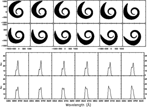
The images (upper panel) of the illuminated area of the disc and Hα line profiles (lower panel) computed by our code for twist warped disc cases for i= 8°, n₁= 2.1π, n₂= 3.0, n₃= 6°, the disc zone is from R_in= 250r_g to R_out= 1000r_g for a retrograde disc. The longitude of the observer γ₀ with respect to the coordinate system of the disc from top left-hand side to bottom right-hand side takes steps of 10° from 50° to 160°. The variation of the line profiles with respect to different longitude can be compared with successive observation of source SDSS J093653.84+533126.8.

Open in new tabDownload slide

4 SUMMARY

We compute the reprocessing emission-line profiles from a warped relativistic accretion disc around a central black hole by including all relativistic effects. A parametrized disc model is used to obtain an insight into the impact of disc warping on the double-peaked Balmer emission-line profiles. For simplicity, we assumed that the disc is illuminated by a point-like central source, which is a good approximation, the line emissivity is proportional to the continuum light intercepted by the accretion disc, and line emission is isotropic. We find the following.

• For twist-free or low phase amplitude (described by n₁) warped disc, the asymmetrical and frequency-shifted single-peaked line profiles as expected are produced in most cases. The rarity of such sources suggests that a warping disc is usually twisted.

• The flux ratio of the blue peak to red one becoming less than unity can be predicted by a twisted warp disc with high phase amplitude. The phase amplitude has a significant influence on the line profiles.

• A third peak and the variation in blue/red peak position which have been found by observations (Veilleux & Zheng 1991; Strateva et al. 2003) are produced in our model.

• The influence from retrograde disc on line profiles has a inverse effect compared with a prograde one.

• The fraction of the radiation incident to the outer disc from the inner part can be enhanced by disc warping. The results are shown in Fig. 5.

We showed that warped disc model is flexible enough to reproduce a variety of line profiles including triplet-peaked line profiles, or double-peaked profiles with additional plateaus in the line wing as observed in the SDSS spectra of some AGN, while the models have the same number of free parameters as eccentric disc models. While we leave the detailed fit to a future paper, the essential characteristics in the line profiles is in good agreement with observed line profiles. Future monitoring of line profile variability in these triplet sources can provide a critical test of the warped disc model.

We would like to thank the anonymous referee for his/her helpful suggestions and comments which helped to improve and clarify our paper.

REFERENCES