The metallicity extremes of the Sagittarius dSph: SALT spectroscopy of PNe* Free

Abstract

1 INTRODUCTION

The most common morphological type of the dwarf galaxies in the Local Group (LG) are the dwarf spheroidals (dSphs). They are also the least massive, least luminous and most gas-deficient galaxies in the LG. The dSph galaxies are mostly found as satellites of larger galaxies, and their properties are likely affected by their dominant neighbours. The main characteristics are a small size, a lack of interstellar gas and young stars, and a range of metallicities that extend to comparatively high values for their luminosity. The causes of these properties are disputed (Grebel, Gallagher & Harbeck 2003). Gas stripping by ram pressure is likely to be involved, and the steep increase of metallicity with age could be caused by removal of the primordial gas reservoir and/or accretion of metal-rich gas from the large neighbour (e.g. Zijlstra et al. 2006).

In gas-deficient galaxies, accurate nebular abundances can still be obtained from spectra of planetary nebulae (PNe). These provide information on elements that are not easily observed in stellar absorption-line spectra. For the LG and other nearby galaxies these abundance data can also be combined with star formation histories derived from colour–magnitude diagrams of resolved stars and ideally with stellar spectroscopic metallicities (e.g. Koch et al. 2007a,b, and references therein). In turn, this yields deeper insights into galaxy evolution, in particular on the overall chemical evolution of galaxies as a function of time. Only in two dSph galaxies in the LG have PNe been detected and observed to date: two in Fornax (Danziger et al. 1978; Kniazev et al. 2007; Larsen 2008) and four in Sagittarius (Zijlstra & Walsh 1996; Zijlstra et al. 2006).

With a heliocentric distance of ∼26 kpc to its central region (Monaco et al. 2004), the Sagittarius dwarf is the closest known dSph. Sgr was discovered by Ibata, Gilmore & Irvin (1994, 1995). It is strongly disrupted by its interaction with the Milky Way (Dohm-Palmer et al. 2001; Helmi & White 2001; Majewski et al. 2003; Newberg et al. 2003; Putman et al. 2004). Since Sgr is located behind the rich stellar population of the Galactic bulge, studies of the stellar population in this galaxy are difficult. Marconi et al. (1998) found that individual stars in Sgr have metallicities in the range −1.58 ≤[Fe/H]≤−0.71. Evidence for a more metal-rich population was presented by Bonifacio et al. (2004), who derived [Fe/H]∼−0.25 based on spectroscopy of 10 red giant stars, while Sbordone et al. (2007) have found even higher metallicities between [Fe/H]=−0.9 and 0. The existence of a significant, much more metal-poor population in Sgr is shown by the metal-poor clusters M 54, Arp 2 and Ter 8 (Layden & Sarajedini 1997,2000).

Zijlstra & Walsh (1996) discovered two PNe in the Sagittarius dwarf spheroidal galaxy that were previously catalogued as Galactic PNe: Wray 16-423 and He 2-436. The first spectroscopy for them was published by Walsh et al. (1997) and a detailed analysis based on ground-based spectra and radio-continuum data was carried out by Dudziak et al. (2000). Two further PNe were analysed in Zijlstra et al. (2006): a Sgr-core member, StWr 2-21, and a possible leading-tail member, BoBn 1. The first two PNe showed identical abundances, of [Fe/H]=−0.55 ± 0.05 (Walsh et al. 1997; Dudziak et al. 2000). The abundances of the two recent objects are less well defined, being based on less accurate spectroscopy. However, current results indicate that one shows a very high abundance for a dwarf galaxy ([Fe/H]≈−0.25), while the other, in contrast, has one of the lowest abundances of any known PN ([Fe/H]≈−2). BoBn 1 is located towards a tidal tail (Zijlstra et al. 2006), but its association with Sgr is not as secure as that of the other three; it could also be an unrelated Galactic halo object.

The goal of our present work is to improve our knowledge of the elemental abundances of the last two PNe in the Sagittarius dSph through new high-quality spectra obtained with the new effectively 8-m diameter Southern African Large Telescope (SALT). The contents of this paper are organized as follows. Section 2 gives the description of all observations and data reduction. In Section 3 we present our results, and discuss them in Section 4. The conclusions drawn from this study are summarized in Section 5.

2 OBSERVATIONS AND DATA REDUCTION

2.1 SALT spectroscopic observations

The observations of StWr 2-21 and BoBn 1 were obtained during the performance-verification (PV) phase of the SALT telescope (Buckley, Swart & Meiring 2006; O'Donoghue et al. 2006), and used the Robert Stobie Spectrograph (RSS; Burgh et al. 2003; Kobulnicky et al. 2003). The long-slit spectroscopy mode of the RSS was used, with three mosaicked 2048 × 4096 CCD detectors. The RSS pixel scale is 0.129 arcsec and the effective field of view is 8 arcmin in diameter. We utilized a binning factor of 2 to give a final spatial sampling of 0.258 arcsec pixel⁻¹. The volume phase holographic (VPH) grating GR900 was used in two spectral ranges: 3500–6600 Å and 5900–8930 Å with a final reciprocal dispersion of ∼0.95 Å pixel⁻¹ and spectral resolution full width at half-maximum (FWHM) of 5–6 Å. Each exposure was observed with the spectrograph slit aligned to the parallactic angle to avoid loss of light due to atmospheric differential refraction. As shown in Table 1, each exposure was broken up into 2–3 subexposures, 10 min each, to allow for removal of cosmic rays. Spectra of ThAr and Xe comparison arcs were obtained to calibrate the wavelength scale. Four spectrophotometric standard stars G 93-48, EG 21, BPM 16274 and SA95-42 (Stone & Baldwin 1983; Baldwin & Stone 1984; Massey et al. 1988; Oke 1990) were observed at the parallactic angles for relative flux calibration.

2.2 Data reduction

The data for each CCD detector were bias and overscan subtracted, gain corrected, trimmed and cross-talk corrected. After that they were mosaicked. The primary data reduction was done using the iraf1 package salt2 developed for SALT data. Cosmic ray removal was done with the task FILTER/COSMIC task in midas.3 We used the iraf software tasks in twodspec package to perform the wavelength calibration and to correct each frame for distortion and tilt. To derive the sensitivity curve, we fitted the observed spectral energy distribution of the standard stars by a low-order polynomial. All sensitivity curves observed during each night were compared and we found the final curves to have a precision better than 2–3 per cent over the whole optical range, except for the region blueward of λ3700 where precision decreases to 10–15 per cent. Spectra were corrected for the sensitivity curve using the Sutherland extinction curve. 1D spectra were then extracted using the iraf APALL task. All 1D spectra obtained with the same setup for the same object were then averaged. Finally, the blue and red parts of the total spectrum of BoBn 1 were combined. The resulting reduced spectra of StWr 2-21 and BoBn 1 are shown in Figs 1 and 2, respectively.

Figure 1

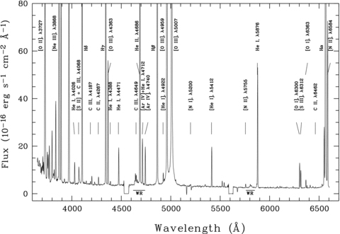
1D reduced spectrum of the planetary nebula StWr 2-21. The spectrum covers the wavelength range 3500–6630 Å. Most of the detected stronger emission lines are marked. All detected lines are listed in Table 2. The locations of detected stellar WR lines are also indicated.

Open in new tabDownload slide

Figure 2

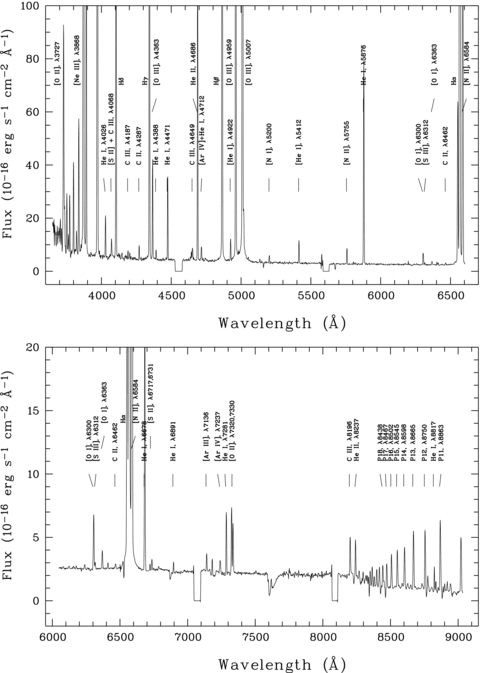
The 1D reduced spectra of the planetary nebula BoBn 1. The top spectrum covers a wavelength range of 3500–6630 Å and bottom spectrum covers a wavelength range of 6000–9050 Å. Most of the detected strong emission lines are marked. All detected lines are listed in Table 2.

Open in new tabDownload slide

All emission lines were measured applying the midas programs described in detail in Kniazev et al. (2000,2004). (1) The software is based on the midas Command Language. (2) The continuum noise estimation was done using the absolute median deviation (AMD) estimator. (3) The continuum was determined with the algorithm from Shergin, Kniazev & Lipovetsky (1996). (4) The programs dealing with the fitting of emission/absorption line parameters are based on the midas FIT package. (5) Every line was fitted with the corrected Gauss–Newton method as a single Gaussian superimposed on the continuum-subtracted spectrum. All overlapping lines were fitted simultaneously as a blend of two or more Gaussian features: the [O i]λ6300 and [S iii]λ6312, the Hαλ6563 and [N ii]λλ6548, 6584 lines, the [S ii]λλ6716, 6731 lines and the [O ii]λλ7320, 7330 lines. (6) The final errors in the line intensities, σ_tot, include two components: σ_p, due to the Poisson statistics of line photon flux, and σ_c, the error resulting from the creation of the underlying continuum and calculated using the AMD estimator. (7) All uncertainties were then propagated in the calculation of errors in electron number densities, electron temperatures and element abundances.

For the Wolf–Rayet (WR) features the Gaussian decomposition to the narrow lines and the broad components was also done using the same method.

SALT is a telescope with a variable pupil, where the illuminating beam changes continuously during the observations. This means that absolute flux calibration is not possible even using spectrophotometric standard stars. To calibrate absolute fluxes we used Hβ fluxes from other sources. For the Hβ flux calibration of BoBn 1 we used the mean value 3.57 × 10⁻¹³erg cm⁻²s⁻¹ calculated from Kwitter & Henry (1996) and Wright, Corradi & Perinotto (2005) which are in close agreement to each other. The value for the Hβ flux from Peña, Torres-Peimbert & Ruiz (1991)(2.19 × 10⁻¹³erg cm⁻²s⁻¹) is about 1.5 times weaker compared to the previous references and was ignored for this reason. For the Hβ flux calibration of StWr 2-21 we used the mean value 1.15 × 10⁻¹³erg cm⁻²s⁻¹ from Zijlstra et al. (2006). The resulting spectra in Figs 1 and 2 are shown after this calibration was performed.

2.3 Physical conditions and determination of heavy-element abundances

The spectra are interpreted by the technique of plasma diagnostics, i.e. assuming that all lines are produced in an isothermal gas at uniform density and ionization level. As a first step, the reddening correction, electron temperatures and density were calculated. These steps are repeated several times, until the values converge.

The measured emission line intensities F(λ) were corrected for reddening using the equation

1

where C(Hβ) is the extinction coefficient, I(λ) is the intrinsic line flux and F(λ) is the observed line flux corrected for atmospheric extinction. F(λ) is the reddening function, taken from Whitford (1958) and normalized at Hβ. Izotov, Thuan & Lipovetsky (1994) noted that this reddening function can be approximated over the whole spectral range with an accuracy better than 5 per cent by

2

where λ is in units of μm. The Balmer theoretical ratios from Brocklehurst (1971) were used with equation (1) in an iterative way for the intrinsic hydrogen line intensity ratios for estimated electron temperature.

For collisionally excited lines (CELs), we calculated ionic and total element abundances for O, N, S, Ne, Ar, Cl and Fe using equations from Izotov et al. (2006). These recent equations are based on sequences of photoionization models and used the new atomic data of Stasińska (2005).

Izotov et al. (2006) find that the electron temperature T_e (O iii) derived from the [O iii](λ4959 +λ5007)/λ4363 line ratio using old and new emissivities differ by less than 1 per cent in the temperature range 5000–20 000 K. For this reason the electron temperature T_e(O iii) was derived from an iterative procedure, using the equation from Aller (1984):

3

where t= 10⁻⁴T_e(O iii) and x= 10⁻⁴N_et^−0.5. The parameters C_T, a₁, a₂ were calculated using the following interpolations:

4

5

6

The density N_e was also derived iteratively, using the [S ii]λ6717/λ6731 line ratio. The [O iii] auroral λ4363 line was corrected for recombination excitation following the equation from Liu et al. (2000).

The line [N ii]λ5755 was detected in the spectra of both studied PNe, which allowed us to determine T_e(N ii) directly from the Q_N=[N II] (λ6548 +λ6584)/λ5755 line ratio. It is convenient to have an analytic expression linked the electron temperature T_e(N ii) to the value of the Q_N and the electron density N_e. To establish such a relation we have obtained the five-level-atom solution for the N⁺ ion, with a recent atomic data. The Einstein coefficients for spontaneous transitions and the energy levels for five low-lying levels were taken from Galavís, Mendoza & Zeippen (1997). The effective cross-sections or effective collision strengths for electron impact were taken from Hudson & Bell (2005). The effective cross-sections are continuous functions of temperatures, tabulated by Hudson & Bell (2005) at a fixed temperatures. The actual effective cross-sections for a given electron temperature are derived from two-order polynomial fits of the data from Hudson & Bell (2005) as a function of temperature.

We derived a numerical solution of the five-level-atom for a large range of values of electron temperature (within the range 5000–25 000 K) and of electron density (within the range 10–10⁶cm⁻³). The analytic relation was derived as an approximation of those numerical results. The following simple expression for the approximation was adopted (this type of expression was widely used by different authors)

7

where t= 10⁻⁴T_e(N ii) and coefficients C_i can be a function of the electron density. At N_e≲ 10³cm⁻³ the coefficients C_i are, in fact, independent of N_e, and the numerical results are well reproduced by the relation

8

derived by Pilyugin (2007) for N_e= 100 cm⁻³. At N_e≳ 10³cm⁻³ the dependence of the coefficients C_i on the electron density are reproduced by the following relations:

9

10

11

12

where w= log (N_e). The values of T_e(N ii) derived directly from the numerical solution and with the approximation differ by less than 3 per cent at N_e≲ 10⁵cm⁻³ and by around 5 per cent at N_e∼ 10⁶cm⁻³ and t ∼ 2.5. It should be emphasized that at N_e≲ 10³cm⁻³equations (9)–(12) are not workable, and equation (8) should be used in this case.

We thus used T_e(N ii) from equation (7) for the calculation of N⁺/H⁺, O⁺/H⁺, S⁺/H⁺ and Fe²⁺/H⁺ abundances. We calculated also T_e(O ii) and T_e(S iii) using approximations from Izotov et al. (2006). We used T_e(S iii) for the calculation of S²⁺/H⁺, Cl²⁺/H⁺ and Ar²⁺/H⁺ abundances and T_e(O iii) from equation (3) for the calculation of O²⁺/H⁺ and Ne²⁺/H⁺ abundances.

For StWr 2-21 only the [O ii]λλ3727, 3729 doublet was used to calculate O⁺/H⁺. In case of BoBn 1, O⁺/H⁺ was calculated as a weighted average of O⁺/H⁺ using intensities of the [O ii]λλ3727, 3729 doublet as well as using the [O ii]λλ7320, 7330 lines. The contribution to the intensities of the [O ii]λλ7320, 7330 lines due to recombination was taken into account following the correction from Liu et al. (2000).

The detection of a strong nebular He iiλ4686 emission implies the presence of a non-negligible amount of O³⁺. In this case its abundance is derived from the relation

13

After that, the total oxygen abundance is equal to

14

From measured intensities of optical recombination lines (ORLs), ionic abundances were calculated using the equation

15

where I_jk/I_Hβ is the intensity ratio of the ionic line to the Hβ line, λ_jk/λ_Hβ is the wavelength ratio of the ionic line to Hβ, α_Hβ is the effective recombination coefficient for Hβ and α_jk is the effective recombination coefficient for the ionic ORL. Ionic abundances derived from ORLs depend only weakly on the adopted temperature and are essentially independent of N_e. A temperature of T_e(O iii) was assumed throughout. The ionic abundance of observed C ii recombination lines was derived using calculated effective recombination coefficients from Davey, Storey & Kisielius (2000), which include both radiative and dielectronic recombination processes. The ionic abundance of observed C iii recombination lines was derived using effective recombination coefficients from Péquignot, Petitjean & Boisson (1991). The effective recombination coefficient for Hβ was taken from Péquignot et al. (1991) as well. Dielectronic recombination coefficients for C iii lines were taken from Nussbaumer & Storey (1984). ICF for C were calculated using Kingsburg & Barlow (1994).

Helium was calculated in the manner described in Izotov, Thuan & Lipovetsky (1997); Izotov & Thuan (1998,2004). The new Benjamin, Skillman & Smith (2002) fits were used to convert He i emission line strengths to singly ionized helium y⁺= He⁺/H⁺ abundances.

The [Cl iii]λ5518/λ5538 line ratio and [Ar iv]λ4711/λ4740 line ratio were also used to calculate the density for StWr 2-21. The TEMDEN task contained within the iraf NEBULAR package was used in this case. Since [Ar iv]λ4711 is contaminated by the He iλ4713 line, we have subtracted the latter adopting a He iλ4713/λ4471 recombination ratio (Brocklehurst 1972) that could be approximated for T_e varying between 10 000 and 20 000 K with a linear equation:

16

Unfortunately, these lines are very weak and have large errors in case of BoBn 1.

3 RESULTS

The measured heliocentric radial velocities for the two studied PNe are given in Table 1. The two independent measurements for BoBn 1 are consistent with each other and all measured velocities are consistent within the uncertainties with velocities published in Zijlstra et al. (2006).

Tables 2 and 3 list the relative intensities of all detected emission lines relative to Hβ[F(λ)/F(Hβ)], the ratios corrected for the extinction [I(λ)/I(Hβ)], as well as the derived extinction coefficient C(Hβ), and the equivalent width of the Hβ emission line EW(Hβ). C(Hβ) combines the internal extinction in each PN and the foreground extinction in the Milky Way, however internal extinction tends to be low in all but the youngest PNe. The electron temperatures T_e(O iii), T_e(N ii), the number densities N_e(S ii), N_e(Ar iv), N_e(Cl iii) are shown in Table 4 together with the line ratios that were used for their calculations. The ionic and total element abundances and ICFs for O, N, Ne, S, Ar, Fe, Cl, C and He are presented in Table 5.

It is desirable to compare densities derived from diagnostics that are observed in the same spectrum, in order to compare the same volume in the nebula. Stanghellini & Kaler (1989) examined densities derived for a large sample of PNe and have found that densities derived from the [O ii], [S ii], [Ar iv] and [Cl iii] doublet ratios agree to within ∼30 per cent. Kingsburg & English (1992) studied a sample of 57 PNe having densities in the range 500–10 000 sm⁻³ and showed that N_e(O ii) and N_e(S ii) are the same within the errors. As seen from Table 4, both PNe have densities that are equal within the formal observational errors and we may conclude that the nebulae are roughly homogeneous.

The comparison of measured line intensities for StWr 2-21 with those published by Zijlstra et al. (2006) show good agreement, within the cited errors. Our RSS spectra have a spectral resolution of 5–6 Å, which is about two times better than the spectral resolution of 11 ÅZijlstra et al. (2006) obtained with EFOSC2 on the ESO 3.6-m telescope. This allows for a more accurate detection of faint lines in the same spectral region and the possibility to fit in detail (see Fig. 1) both the blue and the red WR bumps clearly evident in our spectrum (see Section 3.1 for more details). There are many weak He lines detected in the spectrum of StWr 2-21, especially in the spectral region 5800–6550 Å. Since our observed spectral region for StWr 2-21 is limited to <6630 Å and our detected intensities for the relatively bright lines are very similar to those cited in Zijlstra et al. (2006, see their table 2), we additionally used those spectral data (for λ > 6630 Å) in our calculations of abundances of S, Ar and He. All these lines are marked in Table 3. The determined abundances of various elements using the SALT spectrum are fairly consistent with those published by Zijlstra et al. (2006) that have been obtained from models. Zijlstra et al. (2006) did not determine errors on their abundances. Our data also allow us, for the first time, to determine abundances of Fe and Cl in StWr 2-21.

Torres-Peimbert & Peimbert (1979), Barker (1980), Peña et al. (1991) and Wright et al. (2005) carried out previous spectroscopic observations of BoBn 1 PN using KPNO 2.1-m, CTIO 4-m and INT 2.5-m telescopes. Our data for BoBn 1 are considerably better than the earlier spectra, in terms of signal-to-noise ratio, resolution and spectral coverage, yielding a signal-to-noise ratio, for example, of 23 for the [O iii]λ4363 line. With our new SALT data we securely detect, for the first time, the weak [S ii]λλ6717, 6731 lines [I(6717+6731) ≈ 0.0025 I(Hβ)] and determine the electron number density to be three times as large as found before (Torres-Peimbert & Peimbert 1979; Peña et al. 1991). Unfortunately, even with our data the errors for [S ii]λλ6717, 6731 lines are still large, yielding large errors for the density. This leads to significant errors of practically all calculated abundances based on CELs. Our abundances for BoBn 1 are consistent within the uncertainties cited by (Peña et al. 1991). Abundances for BoBn 1 have been also obtained by Howard, Henry & McCartney (1997) and by Zijlstra et al. (2006) from models. However, both papers are based on the previous observational data (mainly from Peña et al. 1991), where the most important lines for determination of Ar, S and C were obtained with large uncertainties, the [N ii]λ5755 line was outside of the observed spectral region and [S iii]λ6312 was not detected.

The dichotomy between the ORL and CEL abundances is a well-known problem in nebular astrophysics (see Liu 2003, and references therein). Heavy-element abundances derived from ORLs are systematically higher than those derived from CELs. Torres-Peimbert & Peimbert (1979) calculated the abundance of C for BoBn 1 using the ultraviolet C iii]λ1909, comparing it with the C abundance calculated from ORLs and found agreement. Our total C abundance (see Table 5) derived using the five ORL C ii and C iii lines is consistent, within the quoted uncertainties, with their value of 12 + log(C/H) = 9.16 ± 0.15. Unfortunately, there were no ORL lines detected for other elements and we have to conclude that a higher S/N spectrum will be needed to identify any discrepancy between the ORL and CEL abundances for both StWr 2-21 and BoBn 1.

3.1 Wolf–Rayet features

Zijlstra et al. (2006) reported a detection, based on spectral synthesis, of two broad WR features at 3820 and 5805 Å in their StWr 2-21 spectrum. There is confirming evidence in our SALT data of broad blue (4640–4750 Å) and red (5750–5900 Å) WR bumps as it is shown on Fig. 3. We attempted to confirm the detection of broad WR features in our StWr 2-21 spectrum, and if possible to infer their properties.

Figure 3

Gaussian multicomponent fitting of the blue (top) and the red (bottom) WR bumps of StWr 2-21. In the top part of each panel the observed spectrum in the fitted region (dashed lines), fitted Gaussians and created continuum level are shown. In the bottom part of each panel residuals between the observed spectrum and the continuum plus fitted lines are plotted. The following lines from left- to right-hand side are separated. Top panel: The narrow lines (FWHM = 4.1 Å) N iiiλ4634, N iiiλ4640, C iiiλλ4647+4650, [Fe iii]λ4658, He iiλ4686 (narrow and broad components), narrow [Ar iv]+He iiλλ4711+4713 and [Ar iv]λ4740. Bottom panel: The narrow lines (FWHM = 5.15 Å) [N ii]λ5755, C ivλ5801 and C ivλ5812, He iiλ5869 and He iλ5876. Also the broad WR bump C iv was fitted with the centre at λ5805.

Open in new tabDownload slide

The analysis methods used are the same as those described in Section 2.2. A local underlying continuum at all the studied regions was defined for the total spectrum using the algorithm from Shergin et al. (1996). The continuum-subtracted spectral region of each studied spectral region was fitted simultaneously as a blend of a single wide and many narrow Gaussian features. Wavelengths of the narrow Gaussian features used were selected from the list of emission lines located at the respective spectral regions. This list was created by the authors and used by programs described in Section 2.2 for automatic measuring of emission lines. The exact wavelengths of the narrow emission lines were kept fixed during the fitting procedure. During this procedure, the FWHMs of most narrow emission lines were equal to each other, and equal to the FWHM of the strongest narrow emission line observed in the studied region, namely He iiλ4686 for the blue WR bump spectral region and He iλ5876 for the red WR bump region. The FWHM of the strongest narrow emission line, the FWHM of the broad component and its position, and the intensities of all emission lines were used as free parameters during the fitting procedure. Any Gaussian feature was formally detected if the derived intensity was greater than the total error found for this line (signal-to-noise ratio > 1). Gaussian features with detected signal-to-noise ratios less than unity were excluded, and the fitting procedure was repeated.

The results from the fitting procedures and residuals are shown in Fig. 3, while final intensities of all narrow emission lines are given in Table 2. It seems that the WR wide components are indeed present and have the following parameters resulting from the fitting procedure described above: (1) the broad component of the He iiλ4686 line (EW = 16 ± 5 Å, FWHM = 35 ± 15 Å, flux = 58 × 10⁻¹⁶erg s⁻¹cm⁻²); (2) the broad component of C iv centred at λ5805 (EW = 9 Å, FWHM = 42 ± 3 Å, flux = 22 × 10⁻¹⁶erg s⁻¹cm⁻²). Our fitting method is too unstable in the region of the O viλ3822 feature, found previously by Zijlstra et al. (2006), to make any definitive conclusions of its existence in our data.

Both of the broad features which were found, and reported above, show the same velocity range of ≈2200 km s⁻¹. The resulting detected line ratio He iiλ4686/C IV λ5805 ≈ 2.6 supports the conclusion of Zijlstra et al. (2006) that the central star of StWr 2-21 is a hot star midway between subclasses 2 and 3 ([WO 2–3]) according to the classification by Acker & Neiner (2003). The FWHMs of the detected broad lines also fit well those shown in Acker & Neiner (2003) for [WO 2–3] subclasses. No broad WR features were detected in the spectrum of BoBn 1 using the described fitting method.

Finally, four out of six PNe studied in dSphs (Walsh et al. 1997; Zijlstra et al. 2006; Kniazev et al. 2007; Larsen 2008, this work) show WR features in their spectra. This fraction (67 per cent) is much higher than the fraction of [WR]-type central PNe stars in both the Galactic disc (∼6.5 per cent) and the Galactic bulge (∼18 per cent; Górny 2001; Górny et al. 2004). This high fraction of [WR]-type of central PNe stars, as noted by Zijlstra et al. (2006), supports models in which the probability of star to develop a WR wind is determined by parameters of the progenitor star rather than models where this occurrence is a random event caused by a late thermal pulse (Gesicki et al. 2006).

4 DISCUSSION

4.1 Additional enrichment in PN progenitors

H ii region abundances mainly provide information about α-process elements, which are produced predominantly in short-lived massive stars. Because of their common origin, log(Ne/O), log(S/O) and log(Ar/O) should be constant and show no dependence on the oxygen abundance. Izotov & Thuan (1999) very accurately measured these α-element-to-oxygen abundance ratios in a large sample of H ii regions in blue compact galaxies. They found that log(Ne/O) =−0.72 ± 0.06, log(S/O) =−1.55 ± 0.06 and log(Ar/O) =−2.27 ± 0.10, as shown in Fig. 4. Recent spectrophotometric results of Izotov et al. (2006) for a large sample of H ii galaxies from the Sloan Digital Sky Survey DR3 data (Abazajian et al. 2005) support this conclusion. In addition, they found no significant trends with the oxygen abundance for the log(Cl/O) ratio. Using their published data we calculated weighted mean for the log(Cl/O) ratio as −3.46 ± 0.14 and plot these data in the bottom panel of Fig. 4.

Figure 4

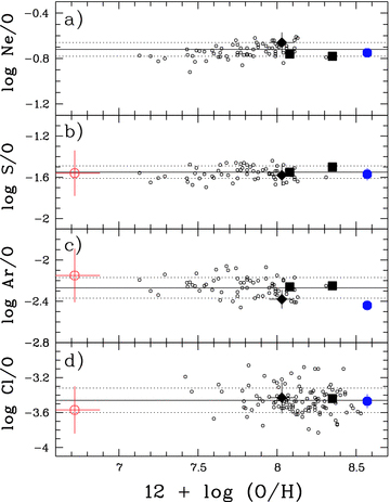
α-element-to-oxygen abundance ratios for log(Ne/O), log(S/O), log(Ar/O) and log(Cl/O) for H ii regions with their 1σ errors (short-dashed lines) as a function of oxygen abundance (Izotov & Thuan 1999; Izotov et al. 2006). Data from Izotov & Thuan (1999), Kniazev et al. (2003), Izotov et al. (2006) are overplotted. Data for PNe in Fornax (filled diamond) and in the Sagittarius dSph galaxies are shown with their 1σ errors. Ratios for PN in Fornax are corrected for self-pollution in oxygen by 0.27 dex (Kniazev et al. 2007). Ratios shown for BoBn 1 in Sgr are corrected for self-pollution in oxygen by 1.09 dex as discussed in Section 4.1, and are plotted as open circles. Data for StWr 2-21 from current work are plotted as filled circles. Data for two PNe in the Sagittarius dSph galaxy from Walsh et al. (1997) were recalculated in the same way as described in Section 2.3 and are plotted as filled squares.

Open in new tabDownload slide

In contrast to H ii regions, some elemental abundances in PNe are affected by the nucleosynthesis in the PN progenitors. Newly synthesized material can be dredged up by convection in the envelope, significantly altering abundances of He, C and N in the surface layers during the evolution of the PN progenitor stars on the giant branch and asymptotic giant branch (AGB). Also a certain amount of oxygen can be mixed in during the thermally pulsing phase of AGB evolution (Kingsburg & Barlow 1994; Péquignot et al. 2000; Leisy & Dennefeld 2006). In combination, it means that only the Ne, S, Cl and Ar abundances, observed in both H ii regions and PNe, can be considered as reliable probes of the enrichment history of galaxies, unaffected by the immediately preceding nucleosynthesis in the progenitor stars. Kniazev et al. (2005) compared observed α-element-to-oxygen abundance ratios to ones for H ii regions, to estimate additional enrichment in oxygen for Type I PN in the nearby galaxy Sextans A. These authors found significant self-pollution of the PN progenitor, by a factor of ∼10 in oxygen. Kniazev et al. (2007) used the same idea during a study of PN in the Fornax dSph galaxy and found that systematically lower ratios for log(S/O), log(Ar/O) and log(Ne/O) in this nebula can be easily explained with additional enrichment in oxygen by 0.27 ± 0.10 dex. After correction for this additional enrichment, all studied ratios increased to the values defined for H ii regions, as shown in Fig. 4. This conclusion is additionally supported by the fact that using the same correction for the observed log(Cl/O) ratio in the Fornax PN, moved the value to −3.41, consistent with the H ii regions [see panel (d) of Fig. 4].

BoBn 1 in Sgr has a complicated abundance pattern, which are hard to show in Fig. 4, since the differences are about 0.9 dex for log(S/O), log(Ar/O) and log(Cl/O) ratios but −0.9 dex for log(Ne/O). We will try to explain neon overabundance for BoBn 1 in Section 4.3 below. However, to explain the lower log(S/O), log(Ar/O) and log(Cl/O) ratios it is natural to suggest just an additional enrichment in oxygen, following Péquignot et al. (2000) and Kniazev et al. (2005,2007). Using the abundance ratios for H ii regions and our observed ratios, this self-pollution can be calculated as the weighted average, δO = 1.09 ± 0.13 dex. After the correction the resulting oxygen abundance 12 + log(O/H) is 6.72 ± 0.16 dex, that is, 1/110 the solar value (Lodders 2003), similar to the metallicity of the old globular cluster Terzan 8 in Sgr (Da Costa & Armandroff 1995). The corrected ratios (shown in Fig. 4 as open circles) are log(S/O) _corr=−1.54 ± 0.11, log(Ar/O) _corr=−2.25 ± 0.12 and log(Cl/O) _corr=−3.62 ± 0.23, consistent with the values in H ii regions, showing that a change in oxygen suffices. Finally, we can estimate that the PN progenitor in BoBn 1 enriched the ejecta by a factor of ∼12 in oxygen and by a factor of ∼240 in nitrogen.

Three of five PNe in dSph galaxies show observed log(Ne/O), log(S/O), log(Ar/O) and log(Cl/O) ratios consistent with abundance ratios for H ii regions. This implies that oxygen dredge-up affects abundances only under some circumstances. Richer & McCall (2007) analysed the abundances for the sample of bright PNe in dwarf irregular galaxies and also suggested that oxygen is dredged up on occasion, even at very low metallicity. Péquignot et al. (2000) argue that oxygen is a by-product of all third dredge-up, but leads to enrichment only at low metallicity. At solar metallicity, the dredged-up material has lower oxygen abundance than the original gas.

It is uncertain why BoBn 1 would show a 3^rd dredge-up (as evidenced by its carbon-rich nature) while other PNe at similar extreme abundances do not. Rotational mixing might be a reason (Siess, Goriely & Langer 2004). However, if BoBn 1 is a member of Sgr, it can have a younger age and larger progenitor mass than Galactic stars of the same metallicity, which favours the occurrence of third dredge-up.

4.2 Abundance comparison

Table 6 shows the elemental abundance of all known PNe in dSphs relative to the solar abundance of Lodders (2003). Values for He 2-436 and Wray 16-423 are from Dudziak et al. (2000), and for the Fornax PN from Kniazev et al. (2007). Dudziak et al. (2000) found that the abundances of the first two Sgr PNe are identical within their uncertainties (0.05 dex), which provides evidence that their progenitor stars formed in a single star burst event within a well-mixed interstellar medium. This star formation episode is estimated to have taken place 5 Gyr ago (Zijlstra et al. 2006). StWr 2-21 shows significantly higher abundances and likely dates from a more recent event of star formation. All four objects are strongly enriched in carbon, with C/O ratios between 3 and 29.

We find that StWr 2-21 is the most metal-rich PN known for the dwarf spheroidal galaxies. Its [O/H] is similar to that of the few most metal-rich PNe in the Large Magellanic Cloud (Leisy & Dennefeld 2006). It confirms the existence of a metal-rich population in Sgr (Zijlstra et al. 2006), in good agreement with what was found by the spectroscopic analysis of red giants (Bonifacio et al. 2004; Monaco et al. 2005; Sbordone et al. 2007). The lack of nitrogen enrichment shows that the initial mass of the progenitor star was M_i < 2.5 M_⊙ and therefore puts a lower limit to the age of t > 1 Gyr. The N/O versus N/H abundance ratio of StWr 2-21 closely follows the relation for Galactic PNe (Leisy & Dennefeld 2006).

BoBn 1 is, in contrast, the most metal-poor object with well-determined abundances, in Sgr. Zijlstra et al. (2006) argue, based on limited data, that its original abundance was [Fe/H] < −2. We find slightly higher values, with S, Ar, Cl and Fe uniformly indicating an original metallicity of [Fe/H]=−1.9. The low metallicity indicates that it belongs to the old population of Sgr (see also the discussion in Bellazzini, Ferraro & Buonanno 1999). The C/O = 25 is notable, showing that the nebular abundances are affected by extreme self-enrichment. In addition to C, this is also the case for N, O, and, surprisingly, for Ne.

4.3 The neon problem

BoBn 1 shows a very unusual abundance pattern, with neon more abundant by number than oxygen. Oxygen and neon are both produced in Type II supernovae, where they are produced in a fixed ratio. The abundance ratio is Ne/O ∼ 0.18 in a range of environments (Henry 1989; Izotov & Thuan 1999; Izotov et al. 2006; Leisy & Dennefeld 2006), in confirmation of their common origin. Neon is also produced in carbon burning high-mass AGB stars and in high-mass novae, but not in amounts exceeding oxygen. However, significant neon can be produced in the intershell of low-mass AGB stars, and this is the likely origin of the enrichment in BoBn 1. In the large sample of Leisy & Dennefeld (2006), the Ne/O ratio is always less than unity: BoBn 1 is unique, and either shows the result of a rather unusual event, or traces evolution within a rare parameter range like mass and/or metallicity.

The intershell contains the ashes of the preceding hydrogen burning. Following helium ignition, this intershell becomes convective and experiences burning at T∼ 3 × 10⁸K (Herwig 2005). The nitrogen is burned to²²Ne via two α captures. In high-mass stars, hot bottom burning destroys the neon, but in low-mass stars this does not occur and neon increases to 2 per cent by mass (Herwig 2005).

Intershell material is usually exposed only in hydrogen-poor stars, which are likely to have lost their hydrogen layer in a very late thermal pulse. These show significant enhancement in Ne (Werner et al. 2004), in two cases also with low O/Ne. Interestingly, the two cases with low O/Ne also show surface hydrogen, although still with H/He ∼1 by mass.

BoBn 1 shows no evidence for hydrogen depletion, or of a separate hydrogen-poor region, and is therefore probably not related to the hydrogen-poor stars. Its intershell products instead are visible due to dredge-up. The neon abundance in BoBn 1 is about 0.15 per cent by mass, compared to 2 per cent expected in the intershell. This suggests dilution by a factor of 15. Assuming an intershell mass of ∼10⁻²M_⊙ (Herwig 2005) we find that the envelope mass at the time of the mixing would have been ∼0.1 M_⊙. Assuming an initial metallicity of the envelope of 0.01 Z_⊙, we find that the final surface abundances of C, N, O, Ne are dominated by the intershell products, while the helium abundance remains dominated by the original envelope. This can consistently explain the observed abundances. The C/O ratio in the intershell is ∼20 (Iben & MacDonald 1995), which approaches the value seen in BoBn 1.

5 CONCLUSIONS

The first scientific results based on SALT observations were published by O'Donoghue et al. (2006), Woudt et al. (2006) and Brosch et al. (2007), based on imaging data. In this paper we present the first spectrophotometric results obtained with SALT and RSS during their PV phase that emphasize the long-slit capabilities of the RSS for spectrophotometric observations. The quality of our data permits us to measure line ratios of elements not accessible in earlier studies. We measured the electron temperatures, the electron densities and element abundances for O, N, Ne, Ar, S, Cl, Fe, C and He elements in two PNe in the Sagittarius dSph galaxy. These results are presented in several tables and plots. Based on the data and discussion presented in the paper, the following conclusions can be drawn.

1. We confirm that StWr 2-21 is the most metal-rich PN known in any dwarf spheroidal galaxies and has an oxygen abundance of 12 + log(O/H) = 8.57 ± 0.02 dex. This [O/H] shows that Sgr contains a younger stellar population with [Fe/H]≈−0.2, in good agreement with spectroscopic abundance measurements in Sgr stars. The element abundance ratios of Ne, S, Ar and Cl to O for StWr 2-21 are consistent with the expected patterns in H ii regions showing absence of any additional enrichment in oxygen in the PN progenitor. The lack of nitrogen enrichment puts a lower limit to the age of PN progenitor t > 1 Gyr.

2. We obtain an oxygen abundance of 12 + log(O/H) = 7.81 ± 0.09 for BoBn 1. According to our analysis, this value should be corrected downward by 1.09 ± 0.13 dex due to the self-pollution of oxygen by the PNe progenitor. After this correction the element abundance ratios S/O, Ar/O and Cl/O appear in a good overall accord with the trends seen for H ii regions. This implies that the PN progenitor had an oxygen abundance of 12 + log(O/H) = 6.72 ± 0.16 dex, or 1/110 of the solar value, similar to the metallicity of the old globular cluster Terzan 8 in Sgr (Da Costa & Armandroff 1995). BoBn 1 is therefore one of the most metal-poor PNe with well-determined abundances and belongs to the old population of Sgr. During its normal stellar evolution, the PN progenitor enriched the material by a factor of ∼12 in oxygen and by a factor of ∼240 in nitrogen.

3. BoBn 1 shows a very unusual pattern with neon being more abundant by number than oxygen. This neon enrichment could be explained by production of neon in the intershell of low-mass AGB stars. In this case the final surface abundances of C, N, O, Ne are dominated by the intershell products, which can consistently explain the observed abundances.

4. We confirm the existence of WR broad lines in StWr 2-21, but no WR features were detected in the spectrum of BoBn 1. The fraction of [WR]-type central PNe stars is 67 per cent for dSph galaxies, that supports models in which the probability of star to develop a WR wind is determined by parameters of the progenitor star.

We thank the anonymous referee for comments which improved the presentation of the manuscript. This paper was written while AAZ was a sabbatical visitor at the South African Astronomical Observatory in Cape Town; AAZ is grateful for the hospitality. We are grateful for the support of numerous people during the SALT PV phase. LSP acknowledges the partial support of the Cosmomicrophysics programme of the National Academy of Sciences and Space Agency of Ukraine.

REFERENCES