Self-similar solutions for the dynamical condensation of a radiative gas layer

Abstract

1 INTRODUCTION

Thermal instability (TI) is an important physical process in astrophysical environments that are subject to radiative cooling. Fall & Rees (1985) investigated the effect of TI caused by Bremsstrahlung on structure formation at galactic and subgalactic scales. TI also plays an important role in the interstellar medium (ISM). The ISM consists of a diffuse high-temperature phase (warm neutral medium, or WNM) and a clumpy low-temperature phase (cold neutral medium, or CNM) in supersonic turbulence. It is known that the ISM is thermally unstable in the temperature range between these two stable phases; that is, in the range T∼ 300 − 6000 K (Dalgarno & McCray 1972). Koyama & Inutsuka (2000,2002) suggested that the structure of the ISM is provided by the phase transition that is caused by the TI that occurs in a shock-compressed region.

The basic properties of TI were investigated by Field (1965), who investigated the TI of a spatially uniform gas using linear analysis for the unperturbed state in thermal equilibrium. The net cooling function per unit volume and time was assumed to be Λ₀ρ²T^α−Γ₀ρ. Field (1965) showed that gas is isobarically unstable for α < 1 and is isochorically unstable for α < 0. In thermal non-equilibrium, however, where the heating and the cooling rates are not equal in the unperturbed state, the stability condition of TI is different from that in thermal equilibrium. This situation is, for example, generated in a shock-compressed region. Balbus (1986) derived a general criterion for the TI of gas in a non-equilibrium state. A flow dominated by cooling is isobarically unstable for α≲ 2 and is also isochorically unstable for α≲ 1. Therefore, the phase with T∼ 300 − 6000 K is both isobarically and isochorically unstable.

The non-linear evolution of TI has been investigated by many authors (Koyama & Inutsuka 2002; Audit & Hennebelle 2005; Hennebelle & Audit 2007; Heitsch et al. 2006; Vazquez-Semadeni et al. 2007) using multi-dimensional simulations. However, the non-linear behaviour has only been investigated analytically by a few authors, using some simplifications in an attempt to gain a deeper insight into the nature of TI. Meerson (1989) investigated analytic solutions under the isobaric approximation. However, this approximation is valid only in the limit of short or intermediate scales.

In this paper, a new semi-analytic model for the non-linear hydrodynamical evolution of TI for a thermally non-equilibrium gas is considered without the isobaric approximation. Once TI occurs, the density increases dramatically until a thermally stable phase is reached. During this dynamical condensation, the gas is expected to lose its memory of the initial conditions, and is expected to behave in a self-similar manner (Zel'dovich & Raizer 1967; Landau & Lifshitz 1959). In particular, in star formation, self-similar (S-S) solutions for a runaway collapse of a self-gravitating gas have been investigated by many authors (Penston 1969; Larson 1969; Shu 1977; Hunter 1977; Whitworth & Summers 1985; Boily & Lynden-Bell 1995). In this paper, S-S solutions describing dynamical condensation by TI are investigated by assuming a simple cooling rate without self-gravity. A family of S-S solutions that have two asymptotic limits (the isobaric and the isochoric modes) is presented.

In Section 2, we derive the S-S equations, and describe the mathematical characteristics of our S-S equations as well as the numerical methods. In Section 3, our S-S solutions are presented and their properties are discussed. In Section 4, the S-S solutions are compared with the results of one-dimensional numerical simulations. The astrophysical implications of the S-S solutions and the effect of dissipation are also discussed. Our study is summarized in Section 5.

2 FORMULATION

2.1 Basic equations

In this paper, we consider S-S solutions describing runaway condensation in a region where the cooling rate dominates the heating rate. The S-S solutions describe the evolution of the fluid after its memories of initial and boundary conditions have been lost during the runaway condensation. Therefore, the solutions are independent of how a cooling-dominated region forms.

A net cooling rate is considered, where Λ and Γ are the cooling and heating rates per unit volume and time, respectively. In low-density regions, the main cooling process is spontaneous emission by collisionally excited gases. In this situation, the cooling rate is determined by the collision rate, which is proportional to ρ². Therefore, we adopt the following formula as the net cooling rate:

1

where P, c_s, γ and α are the pressure, sound speed, the ratio of specific heat, and a free parameter, respectively. The effects of viscosity and thermal conduction are neglected for simplicity.

The basic equations for a radiative gas under a plane-parallel geometry are the continuity equation,

2

the equation of motion,

3

and the energy equation,

4

where D/Dt=∂/∂t+v∂/∂x indicates the Lagrangian time derivative.

2.2 Derivation of self-similar equations

The density increases infinitely because the net cooling rate is assumed to be ∝ρ²c^2α_s in equation (1). The epoch at which the density becomes infinite is defined by t_c. We introduce a similarity variable ξ and assume that each physical quantity is given in the following form:

5

By assuming a power-law time dependence of x₀(t) =atⁿ_*, where t_*= 1 −t/t_c and n= 1/(1 −ω), we find the following relations:

6

where β=ω(3 − 2α) − 1. Because the dimensional scale is introduced only by Λ₀, the time dependence of the physical quantities cannot be fixed. Therefore, we leave ω as a free parameter.

For convenience, instead of ω, we can use a parameter η, which is given by

7

Using η, the time dependences of ρ₀(t) and P₀(t) are given by

8

Substituting equations (5) and (6) into the basic equations (2), (3) and (4), the similarity equations are obtained as

9

10

and

11

2.3 Homologous special solutions

The similarity equations (9), (10) and (11) have homologous special solutions with a spatially uniform density and sound speed. Substituting Ω(ξ) =Ω₀ and X(ξ) =X₀ into the similarity equations (9), (10) and (11), one obtains

12

13

and

14

Equation (12) can be integrated to give

15

where V(ξ= 0) = 0 is assumed. Substituting equation (15) into equation (13), one obtains

16

Therefore, homologous solutions exist for β= 0, ω= 0 or α= 1. Equation (14) gives the relation between Ω₀ and X₀. For β= 0, the solution is given by Ω(ξ) =Ω₀, V(ξ) = 0 and X(ξ) =X₀. The time dependences of the density and sound speed are given by

17

respectively. This is the homologous isochoric mode. For α≥ 1, the solution is unphysical because the sound speed is negative or complex. Therefore, no homologous isochoric solutions exist for α≥ 1. This fact is related to the Balbus criterion for the isochoric instability (Balbus 1986). The solution with ω= 0 indicates isothermal condensation. For α= 1, no S-S solutions are found except for the homologous solutions as shown in Section 3.

2.4 Asymptotic behaviour

In this subsection, the asymptotic behaviour of the S-S solutions at ξ→∞ and ξ→ 0 is investigated.

2.4.1 Solutions forξ→∞

Assuming that Ω(ξ) is a decreasing function of ξ and that |V(ξ)| and X(ξ) are increasing functions, equations (9), (10) and (11) become

18

to the lowest order. Expanding to the next order, the asymptotic solutions are given by

19

20

and

21

where

22

23

and

24

2.4.2 Solutions forξ→ 0

We expand Ω(ξ), V(ξ) and X(ξ) in the following forms:

and

25

Substituting equations (25) into (9), (10) and (11), we obtain the following relations for the coefficients:

26

The relation between Ω₀₀ and X₀₀ is given by

27

The relation between Ω⁽¹⁾₀₀ and X⁽¹⁾₀₀ is given by

28

and ν is given by

29

2.5 Critical point

Equations (9), (10) and (11) can be rewritten as

30

where

31

32

33

34

and

35

A singular point exists where I₁= 0 in each of the equations (30). This is the critical point (ξ=ξ_s). In the S-S solution which is smooth at this point, the numerators (I₂, I₃ and I₄) must vanish at ξ=ξ_s. Among the four conditions I₁=I₂=I₃=I₄= 0 there are two independent conditions that are given by

36

2.5.1 Topological properties of the critical point

In this subsection, the topological properties of the critical point are investigated. We introduce a new variable s, defined by ds=I₁dξ (Whitworth & Summers 1985). The dimensionless quantities at infinitesimal distances from the critical point, s_s+δs, are given by

37

where Q= (ξ, ln Ω, V, ln X). The subscript ‘s’ indicates the value at the critical point. Substituting equation (37) into equations (30) and linearizing, one obtains

38

The eigenvalues λ of A_ij describe the topology of the critical point. The eigenequation is given by

39

where

40

and

41

where ε_s= (γ− 1)Ω_sX^2(α−1)_s. The degenerate solution, λ= 0, is attributed to the homologous special solutions (see Subsection 2.3). Therefore, the topology is described by the two eigenvalues other than λ= 0.

2.6 Numerical methods

In this subsection, our numerical method for solving the similarity equations (30) is described. We adopt s as an integrating variable. Using s, equations (30) are rewritten as

42

which are not singular at the critical point.

The critical point is specified by (ξ_s, V_s) because there are four unknown quantities Q_s and two conditions, namely equations (36). Moreover, the similarity equations (42) are invariant under the transformation ξ→mξ, V →mV, Ω→m^−2(α−1)Ω and X→mX, where m is an arbitrary constant. Therefore, the S-S solution for (mξ_s, mV_s) is the same as that for (ξ_s, V_s). As one can take m in such a way that (ξ_s, V_s) satisfies the relation ξ²_s+V²_s= 1, the critical point is specified only by ξ_s.

Given ξ_s, the velocity is obtained as ⁠. From equations (36), Ω_s and X_s are determined. As X_s=V_s+ξ_s is positive, the range of ξ_s is ⁠. The similarity equations (42) are integrated from ξ_s in both directions (ξ→ 0 and ξ→∞) along the gradient derived from equation (38) using the fourth-order Runge–Kutta method. The position of the critical point ξ_s is determined iteratively by the bisection method until the solution satisfies the asymptotic behaviours (see Subsection 2.4).

3 RESULTS

3.1 Physically possible range of parameters (η, α)

In this section, we constrain the parameter space (η, α) by the physical properties of the flow.

3.1.1 Range ofη

Using equation (8), the time dependences of the central density and pressure are given by

43

where the subscript ‘00’ indicates the value at the centre. During S-S condensation by cooling, the central density (pressure) must increase (decrease) monotonically with time. Therefore, the following two conditions are obtained:

44

and

45

From equations (44) and (45), the range of η is given by

46

For η∼ 0, the time dependences of ρ₀₀ and P₀₀ are given by

47

This time evolution indicates the isochoric mode. For η∼ 1, the time dependences of ρ₀₀ and P₀₀ are given by

48

corresponding to the isobaric mode. The critical value of η=η_eq is given by the condition that the increasing rate of ρ₀₀(t) is equal to the rate of increase/decrease of P₀₀(t), which is given by

49

For η=η_eq, the time dependences of ρ₀₀ and P₀₀ are given by

50

Therefore, the S-S solutions for 0 < η < η_eq and η_eq < η < 1 are close to the isochoric and the isobaric modes, respectively.

3.1.2 The range ofα

In the similarity equations (42), the critical point is specified by ξ_s for given α and η. The topology of the critical point is given by the two eigenvalues of the eigenequation (39) other than λ= 0. When the two eigenvalues are real and have the same sign, the critical point is a node. When the two eigenvalues are real and have opposite signs, the critical point is a saddle. When the two eigenvalues are complex, the critical point is a spiral. Fig. 1 shows the topology of the critical point in the parameter space (ξ_s, η) for α= 0.3, 0.5, 0.8, 0.9, 1.1 and 1.2. In Fig. 1, the letters ‘N’, ‘SD’ and ‘SP’ indicate a node, a saddle and a spiral, respectively. The open circles indicate the numerically obtained S-S solutions presented in Subsection 3.2. Fig. 1 shows that the topology drastically changes at α= 1. For α < 1, because the critical point is a node or a saddle, the S-S solutions are expected to exist. For α≃ 1.1, a non-negligible fraction of the parameter space is covered by a spiral. Almost all the parameter space is a spiral for α≳ 1.2. We searched the S-S solutions that connect 0 < ξ < ∞ and found them only in N and SD for α < 1.

Figure 1

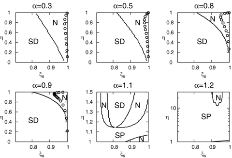
Topological properties of the critical point for α= 0.3, 0.5, 0.8, 0.9, 1.1 and 1.2. The ordinates and abscissas are η and ξ_s, respectively. The letters ‘N’, ‘SD’ and ‘SP’ indicate a node, a saddle and a spiral, respectively. The open circles indicate S-S solutions.

Open in new tabDownload slide

3.2 Self-similar solutions

In this subsection, we describe new S-S solutions and investigate their properties. As shown in Subsection 3.1.1, our S-S solutions exist for 0 < η < 1 and α < 1.

Figs 2(a),(b) and (c) show the obtained S-S solutions for α= 0.5 with η= 0.98, 0.76 and 0.12, respectively. The ordinates denote the dimensionless quantities (Ω, −V, Π, X). The abscissas denote the dimensionless coordinate ξ. The S-S solutions for η= 0.98 and 0.12 approximately represent the isobaric and the isochoric modes, respectively. The solution for η= 0.76 ∼η_eq corresponds to the intermediate mode shown in Subsection 3.1.1. The open circles indicate the critical points. In Figs 2(a),(b) and (c), one can see that the S-S solutions depend strongly on η. Let us focus on the dependence on η of the density and pressure, shown in Figs 2(d) and (e), respectively. In these figures, it can be seen that, for η= 0.98 (the isobaric mode), the density increases sharply towards ξ= 0, whereas the pressure is almost spatially constant. In contrast, for η= 0.12 (the isochoric mode), the density is almost spatially constant whereas the pressure decreases sharply towards ξ= 0.

Figure 2

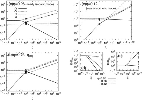
The distribution of dimensionless quantities (Ω, −V, Π, X) for (a) η= 0.98, (b) 0.76 and (c) 0.12. The open circles indicate the critical points. Panels (d) and (e) indicate the dependence of Ω/Ω₀₀ and Π/Π₀₀, respectively, on η.

Open in new tabDownload slide

Next, the S-S solutions are shown using the dimensional physical quantities for various values of η. Fig. 3 shows the time evolution of ρ (first row), P (second row) and −v (third row). The columns in Fig. 3 correspond to η= 0.98, 0.76 and 0.12 from left to right. The solid, long-dashed, short-dashed and dotted lines correspond to t_*= 1, 0.1, 0.01 and 0.001, respectively. From Fig. 3, it can clearly be seen that η specifies how the gas condenses. In the case with η= 0.98 (the isobaric mode), runaway condensation occurs and the density increases in the central region, whereas the pressure is spatially and temporally constant. In the case with η= 0.12 (the isochoric mode), the density is spatially and temporally constant and P₀₀ decreases considerably. In the case with η= 0.76, the condensation occurs in an intermediate manner between the isobaric and the isochoric modes.

Figure 3

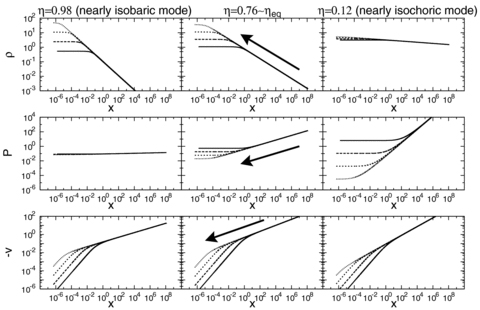
Time evolution of dimensional quantities (ρ, P, −v). The solid, long-dashed, short-dashed and dotted lines correspond to t_*= 1, 0.1, 0.01 and 0.001, respectively. The columns correspond to η= 0.98, 0.76 and 0.12 from left to right, respectively. The arrows indicate the time evolution of flow.

Open in new tabDownload slide

The relevant parameters (η, n, −η/(2 −α), (1 −η)/(1 −α), ξ_s, Ω₀₀, X₀₀, Ω_∞, V_∞, X_∞) for the S-S solutions obtained for α= 0.5 are summarized in Table 1.

From the above results, it is confirmed that the S-S solutions are specified by η and contain two asymptotic limits (the isobaric and the isochoric modes). Moreover, the parameter η is related to the ratio of the sound-crossing to the cooling time-scales in the central region. The time-scales are defined by

51

and

52

where c₀₀ is the sound speed at the centre, and the scale-lengths x_cen(t) and ξ_cen are defined by

53

From equations (51) and (52), the ratio τ of the above two time-scales is obtained as

54

Fig. 4 shows the dependence of τ on η for α=−0.5, 0.5 and 0.8. The figure shows that τ→ 0 for η→ 1 and τ→∞ for η→ 0, independent of α. For η∼ 1, because τ≪ 1, the gas condenses in pressure equilibrium with its surroundings. For η∼ 0, because τ≫ 1, the pressure decreases and the density increases only slightly. These facts are consistent with the discussion in Subsection 3.1.1 and with Fig. 3.

Figure 4

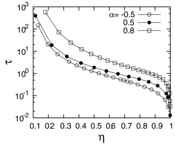
The dependence of τ (equation 54) on η. The open circles, filled circles and open boxes indicate the S-S solutions for α=−0.5, 0.5 and 0.8, respectively.

Open in new tabDownload slide

Finally, we consider the range of α for which the S-S solutions exist. When α= 1.0, no S-S solutions are found except for the homologous special solutions (see Subsection 2.3). Moreover, as mentioned in Subsection 2.3, there are no homologous isochoric solutions for α > 1. Therefore, for α > 1, the condensation of the fluid is not expected to be self-similar. Fouxon et al. (2007) found a family of exact solutions for α= 1.5 > 1. Their solutions are not self-similar because t^cen_sound and t^cen_cool in the central region obey the following different scaling laws: t^cen_sound∝t^3/2_* and t^cen_cool∝t_*. In their solution, during condensation, as t^cen_sound becomes much smaller than t^cen_cool, the pressure of the central region is expected to be constant and the isobaric approximation is locally valid.

4 DISCUSSION

4.1 Comparison with the results of time-dependent numerical hydrodynamics

We compare the S-S solutions with the results of time-dependent numerical hydrodynamics using the one-dimensional Lagrangian second-order Godunov method (van Leer 1997). A converging flow of an initially uniform and thermal-equilibrium gas (ρ(x) =P(x) = 1) is considered. An initial velocity field is given by v(x) =−2 tanh(x/L), where L is a parameter. The net cooling rate is assumed to be ⁠, where α= 0.5. The inflow creates two shock waves, which propagate outwards. Runaway condensation of the perturbation owing to TI occurs in the post-shock region because the cooling rate dominates the heating rate. The central density continues to grow and ultimately becomes infinite. During the runaway condensation, the flow in the central region is expected to lose the memory of the initial and the boundary conditions, and to converge to one of the S-S solutions. The scale of perturbation in the post-shock region can be controlled by the value of L. The larger L is, the larger the scale of perturbation becomes. We perform numerical simulations for L= 0.005, 0.01, 0.02, 0.2 and 0.5.

Fig. 5 shows the time evolution of ρ_cen(t) and P_cen(t) as a function of 1 −t/t_con, where ρ_cen and P_cen are the central density and pressure, and t_con is the epoch at which ρ_cen becomes infinite as estimated from the numerical results. The panels represent (a) L= 0.01, (b) 0.02, (c) 0.2 and (d) 0.5. Using equation (43), the time evolution of ρ_cen(t) and P_cen(t) of each simulation provides the corresponding η. As a result, the corresponding values of η are found to be (a) 0.99, (b) 0.98, (c) 0.76 and (d) 0.50. The thin solid lines in Fig. 5 indicate the corresponding S-S solutions. From the value of η and Fig. 5, cases (a) and (b) correspond to the isobaric mode, case (c) corresponds to the intermediate mode (η∼η_eq), and case (d) corresponds to the isochoric mode. There is a difference in the convergence speed from the corresponding S-S solution. Fig. 5 shows that the convergence speed of (a) and (b) is faster than that of (c) and (d). This is because the scale-length of the condensed region of (a) and (b) is smaller and the sound-crossing time-scale is shorter.

Figure 5

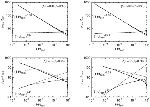
The time evolution of ρ₀₀ (thick lines) and P₀₀ (dashed lines) as a function of 1 −t/t_con for (a) L= 0.01, (b) 0.02, (c) 0.2 and (d) 0.5. The thin solid lines indicate the corresponding S-S solutions.

Open in new tabDownload slide

Fig. 6 shows the time evolution of the rescaled density ρ(1 −t/t_con)^η/(2−α) and pressure P(1 −t/t_con)^{−(1−η)/(1−α)} as a function of the rescaled coordinate x(1 −t/t_con)⁻ⁿ. The parameters L and η in Fig. 6 are the same as those in Fig. 5. The thin solid lines in Fig. 6 indicate the corresponding S-S solutions. In all cases (a–d), the central regions are well approximated by the corresponding S-S solutions. From Fig. 6, it can be seen that the region that is well approximated by the S-S solution spreads with time in each panel.

Figure 6

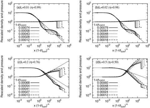
The distribution of the rescaled density ρ(1 −t/t_con)^η/(2−α) and pressure P(1 −t/t_con)^{−(1−η)/(2−α)} as a function of the scaled coordinate x(1 −t/t_con)⁻ⁿ. The L and η in each panel are the same as those in Fig. 5. The lines are labelled according to 1 −t/t_con. The rescaled density and pressure at the centre are set to 10 and 0.1, respectively. The thin solid lines indicate the corresponding S-S solutions.

Open in new tabDownload slide

From the above discussion, the non-linear evolution of perturbation is well approximated by one of the S-S solutions in the high-density limit. Which S-S solution (0 < η < 1) is more likely to be realized in actual environments where various scale perturbations exist? To answer this question, the dependence of t_con on L is investigated. Fig. 7 shows the dependence of 1/t_con on 1/L. Here, 1/L and 1/t_con correspond to the wavenumber and the growth rate of the perturbation, respectively. Therefore, Fig. 7 can be interpreted as an approximate dispersion relation for the non-linear evolution of TI. For larger 1/L, 1/t_con is larger, and 1/t_con appears to approach a certain asymptotic value. A similar behaviour is also found in the dispersion relation of Field (1965) without heat conduction. In Fig. 7, the condensation for 1/L= 5.0 corresponds to the intermediate mode. Furthermore, although the isobaric condensation grows faster, there is little difference between 1/t_con for 1/L= 200 (the isobaric mode) and 2 (the isochoric mode). Therefore, both the isobaric and the isochoric condensations are expected to coexist in actual astrophysical environments.

Figure 7

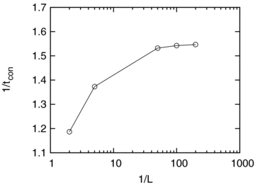
The dependence of the growth rate, 1/t_con, on the wavenumber, 1/L.

Open in new tabDownload slide

4.2 Astrophysical implications

In astrophysical environments, there are roughly two ranges of temperature with α < 1 where our S-S solutions are applicable.

In the high-temperature case, T≳ 2 × 10⁵K (Sutherland & Dopita 1993), the dominant coolants are metal lines and Bremsstrahlung. In a shock with a velocity greater than

55

the post-shock region is thermally unstable (α < 1). For example, a typical supernova satisfies this condition, and S-S condensation is expected to occur. In reality, the density does not become infinite because the cooling time-scale increases when the gas reaches the thermally stable phase. In this case, the cooled layer will rebound and overstability occur (Chevalier & Imamura 1982; Yamada & Nishi 2001; Sutherland, Bicknell & Dopita 2003).

In the low-temperature case, 300 ≲T≲ 6000 K, the dominant coolant is neutral carbon atom. Koyama & Inutsuka (2000) suggested that the structure of the ISM is caused by TI during the phase transition (WNM → CNM). The phase transition is induced by a shock wave. Hennebelle & Perault (1999) considered the converging flow of a WNM under a plane-parallel geometry using one-dimensional hydrodynamical calculations, and investigated the condensation condition of the Mach number and pressure in the pre-shock region. In situations that satisfy their condition, S-S condensation is expected to occur.

4.3 Effects of dissipation

In the actual gas, the effects of viscosity and heat conduction become important on small scales. The importance of dissipation can be evaluated by the ratio between the advection and the dissipation terms, or the Raynolds number, which is given by

56

where C_V, K (T) and U are the specific heat at constant volume, the heat conduction coefficient, and the typical velocity, respectively. The Plandtl number is implicitly assumed to be of order unity. A typical length-scale is assumed to be x_cen(t). If the flow converges to one of the S-S solutions, the ratio, τ, between the sound-crossing and the cooling time-scales is constant. Therefore, τ is defined by

57

Using τ, x_cen is written as

58

Substituting this equation into equation (56), one obtains

59

where U=f_vc₀₀(f_v < 1) and K(T₀₀) =K₀c^κ₀₀.

For the low-temperature case, we adopt (Parker 1953) and the following cooling function (Koyama & Inutsuka 2002):

60

From equation (59), the Raynolds number is given by

61

In the isobaric mode, τ∼ 0.1 from Fig. 4. Because the Raynolds number is much larger than unity, the dynamical condensation of the post-shock region is expected to be well described by the S-S solution with τ≳ 0.1.

For the high-temperature case, the cooling rate of metal lines (10⁵K < T < 10⁷K) is given by

62

We adopt K= 1.24 × 10⁻⁶T^5/2ergs cm⁻¹K⁻¹s⁻¹ (Parker 1953). Using this formula and eqution (59), the Raynolds number is given by

63

Because ⁠, in the high-temperature case the S-S solution with τ≳ 0.1 is expected to describe the dynamical condensation well.

As the temperature decreases, decreases and becomes less than unity at a certain epoch. Thereafter, our S-S solutions are invalid and the effect of dissipation becomes important.

5 SUMMARY

We have provided S-S solutions describing the dynamical condensation of a radiative gas with Λ−Γ∼ρ²T^α. The results of our investigation are summarized as follows.

• Given α, a family of S-S solutions written as equation (8) is found. The S-S solutions have the following two limits. The gas condenses almost isobarically for η∼ 1, and the gas condenses almost isochorically for η∼ 0. The S-S solutions exist for all values of η between the two limits (0 < η < 1). No S-S solutions are found for α > 1.

• The derived S-S solutions are compared with the results of numerical simulations for converging flows. In the case with any scale of perturbation in the post-shock region, our S-S solutions approximate the results of numerical simulations well in the high-density limit. In the post-shock region, smaller-scale perturbations grow faster and asymptotically approach the S-S solutions for η∼ 1. However, the difference of the growth rate between the isobaric mode (η_eq < η < 1) and the isochoric mode (0 < η < η_eq) is small. Therefore, in actual astrophysical environments, the S-S condensations for various η are expected to occur simultaneously.

In the S-S solutions presented in this paper, a plane-parallel geometry is assumed. This situation is much simpler than the two-dimensional simulations that are currently being carried out involving TI, so the results are of limited use, although they may be relevant to code tests that are run on a one-dimensional simulation. The stability analysis on the present S-S solution may provide some insight into the multi-dimensional turbulent velocity field. The effects of the magnetic field and self-gravity may also be important in the ISM, but they are neglected in this paper. These issues will be addressed in forthcoming papers.

This work was supported in part by the 21st Century COE Program ‘Towards a New Basic Science; Depth and Synthesis’ in Osaka University, funded by the Ministry of Education, Science, Sports and Culture of Japan.

REFERENCES