


Abstract
We have used the Sydney University Stellar Interferometer to measure the angular diameter of α Cir. This is the first detailed interferometric study of a rapidly oscillating A (roAp) star, α Cir being the brightest member of its class. We used the new and more accurate Hipparcos parallax to determine the radius to be 1.967 ± 0.066 R⊙. We have constrained the bolometric flux from calibrated spectra to determine an effective temperature of 7420 ± 170 K. This is the first direct determination of the temperature of an roAp star. Our temperature is at the low end of previous estimates, which span over 1000 K and were based on either photometric indices or spectroscopic methods. In addition, we have analysed two high-quality spectra of α Cir, obtained at different rotational phases and we find evidence for the presence of spots. In both spectra we find nearly solar abundances of C, O, Si, Ca and Fe, high abundance of Cr and Mn, while Co, Y, Nd and Eu are overabundant by about 1 dex. The results reported here provide important observational constraints for future studies of the atmospheric structure and pulsation of α Cir.
1 INTRODUCTION
The rapidly oscillating Ap (roAp) stars are chemically peculiar main-sequence stars with effective temperatures around 6500–8000 K. They are found around the classical instability strip but have quite different properties from the δ Scuti stars, due to their slow rotation and strong global magnetic fields (typically of several kilogauss (kG), and up to 24 kG). They have peculiar abundances of Sr, Co and certain rare earth elements such as Eu, Nd, Pr, Tb and Th that are found in high concentration high in the atmosphere (Ryabchikova et al. 2007). The roAp stars present an intriguing possibility to study element stratification, stellar evolution and pulsation in the presence of magnetic fields.
The roAp stars oscillate in high-overtone, low-degree p modes similar in period to the 5-min acoustic oscillations in the Sun, but with coupling of the magnetic field, rotation and the oscillations that must be considered (Cunha 2005). The excitation of high-overtone pulsations, instead of the low overtones found in δ Scuti stars, is thought to be directly related to the strong magnetic fields, which may suppress envelope convection, increasing the efficiency of the opacity mechanism in the region of hydrogen ionization (Balmforth et al. 2001; Cunha 2002). Asymptotic theory, valid for high overtones, predicts that regularly spaced peaks will dominate the frequency spectra of roAp stars, and this has been observed in photometric studies of several stars of the class (Matthews, Kurtz & Martinez 1999). More recently, detailed pulsation studies of roAp stars have used high-resolution spectra collected at high cadence. From analysis of the rare earth element lines a complex picture has emerged, in which the mode amplitudes and sometimes phases depend on atmospheric height, indicating the presence of running magneto-acoustic waves (Kurtz, Elkin & Mathys 2006b; Ryabchikova et al. 2007).
α Circini (HR 5463, HD 128898; V= 3.2) is the brightest of 40 currently known roAp stars. It has one dominant oscillation mode with a period of 6.8 min and a semi-amplitude of 2.5 mmag in B. Four other modes with amplitudes lower by an order of magnitude were detected in an extensive three-site ground-based campaign by Kurtz et al. (1994), but a clear signature of the large separation has so far not been found in the star. Recently, the WIRE satellite observed α Cir which for the first time directly showed the rotational modulation (Prot= 4.46 d) and a clear regular structure of the pulsation peaks, with three modes having comparable amplitudes. The equidistant separation between them has been interpreted as half the large separation (Bruntt et al., in preparation). This new result offers the possibility to confront observations with theoretical evolution and pulsation models for the star.
To make progress in the asteroseismic modelling of α Cir we not only need to measure accurate frequencies with secure mode identification, but also to know with good accuracy the fundamental parameters of the star. It is the goal of the current paper to determine the effective temperature, luminosity, mass and chemical composition of α Cir. A core-wing anomaly is seen in the Balmer lines of Ap stars (Cowley et al. 2001), indicating that the temperature structure is different from normal A-type stars. Therefore, estimates of fundamental parameters from photometric indices or spectral analysis are likely to be affected by systematic effects (Kochukhov, Khan & Shulyak 2005). For example, Teff estimates for α Cir cover the range 7470–8730 K (considering 1σ uncertainties; cf. Table 4), spanning a large part of the range of Teff of the stars belonging to the roAp class. Also, estimating the surface gravity from a classical abundance analysis (e.g. Kupka et al. 1996) by requiring lines of neutral and ionized lines to yield the same abundance is questionable (Ryabchikova et al. 2002).
Fundamental atmospheric parameters of α Cir as found in the literature and the current study.
| Study | T eff (K) | log g | [Fe/H] | Applied method |
| Kurtz & Martinez (1993) | 8000 | H β index | ||
| North et al. (1994) | 8000 | 4.42 | +0.2 | Geneva indices |
| Kupka et al. (1996) | 7900 ± 200 | 4.2 ± 0.15 | −0.13 ± 0.10 | Spectral analysis |
| – | 7950 | 4.3 | Strömgren indices | |
| – | 7880 | 4.4 | +0.3 | Geneva indices |
| Sokolov (1998) | 8440 ± 290 | Continuum slope | ||
| – | 7680 | Geneva indices | ||
| Matthews et al. (1999) | 8000 ± 100 | Hβ index | ||
| Kochukhov & Bagnulo (2006) | 7673 ± 200 | 4.12 ± 0.06 | Geneva indices | |
| This paper | 7420 ± 170 | 4.09 ± 0.08 | Interferometry + bolometric flux | |
| – | −0.12 ± 0.08 | Spectral analysis |
The importance of obtaining accurate fundamental parameters through interferometry for detailed asteroseismic studies was discussed in detail by Creevey et al. (2007) and Cunha et al. (2007). In the current paper we present new interferometric data to measure the angular diameter of α Cir. We use calibrated spectra to estimate the bolometric flux, which in turn allows us to determine the effective temperature nearly independently of atmospheric models. In our companion paper on the detection of the large frequency separation (Bruntt et al., in preparation), we apply the parameters found here in our theoretical modelling of the star.
The presence of strong magnetic fields in roAp stars is thought to suppress the turbulence in their outer atmospheres (Michaud 1970). For this reason, enhanced diffusion leads to stratification of elements (e.g. Babel & Lanz 1992). A more complicated picture was found in the roAp star HR 3831 by Kochukhov et al. (2004), who monitored significant changes in spectral lines with rotational phase. Using a Doppler imaging technique they found rings and spots of different spatial scales, with enhanced abundances up to 7 dex for some elements (see also Lüftinger et al. 2007). Such studies require high-quality data covering a wide range of rotational phases and this has not been done for α Cir. Single spectra indicate that it is a typical roAp star, with high abundances of certain elements such as Co and Nd (Kupka et al. 1996). To confirm the evidence of spots on α Cir found by Kochukhov & Ryabchikova (2001), we present in Section 6 an analysis of two high-resolution and high signal-to-noise ratio (S/N) spectra taken at different rotational phases.
2 OBSERVATIONS AND DATA REDUCTION
The Sydney University Stellar Interferometer (SUSI; Davis et al. 1999) was used to measure the squared visibility, i.e. the normalized squared modulus of the complex visibility or V2, on a total of eight nights. The red-table beam-combination system was employed with a filter of centre wavelength and full width half-maximum (FWHM) 700 and 80 nm, respectively. This system, including the standard SUSI observing procedure, data reduction and calibration, is described by Davis et al. (2007).
Target observations were bracketed with calibration measurements of nearby stars, which were chosen to be essentially unresolved. Using an intrinsic colour interpolation (and spread in data) of measurements made with the Narrabri Stellar Intensity Interferometer (Hanbury Brown, Davis & Allen 1974), the angular diameters (and associated uncertainty) of the calibrator stars were estimated and corrected for the effects of limb darkening. However, post-processing indicated that two of the calibrator stars (HR 4773: γ Mus and HR 5132: ε Cen) are binaries and could not provide adequate calibration information. The adopted stellar parameters of the remaining calibrator stars are given in Table 1. A linear interpolation of the calibrator transfer functions was then used to scale the observed squared visibility of the target. This procedure resulted in a total of 60 estimations of V2 and a summary of each night is given in Table 2.
Adopted parameters of the two calibrator stars. The primary calibrator, β Cir, was used on all nights while the secondary calibrator, σ Lup, was also used on April 22 and July 30.
| HR | Name | Spectral type | V (mag) | UD diameter (mas) | Separation from α Cir |
| 5670 | β Cir | A3 V | 4.05 | 0.58 ± 0.05 | 7°. 42 |
| 5425 | σ Lup | B2 III | 4.42 | 0.20 ± 0.04 | 14°. 59 |
| HR | Name | Spectral type | V (mag) | UD diameter (mas) | Separation from α Cir |
| 5670 | β Cir | A3 V | 4.05 | 0.58 ± 0.05 | 7°. 42 |
| 5425 | σ Lup | B2 III | 4.42 | 0.20 ± 0.04 | 14°. 59 |
Summary of observational interferometry data for α Cir from SUSI. The night of the observation is given in Columns 1 and 2 as a calendar date and the mean MJD −54000. The nominal and mean projected baselines in units of metres are given in Columns 3 and 4, respectively. The weighted-mean squared visibility, associated error and the number of observations during each night are given in the last three columns.
| Date in 2007 | MJD | Nominal baseline | Projected baseline |  |  | N |
| April 18 | 208.62 | 5 | 4.08 | 0.964 | 0.012 | 10 |
| April 20 | 210.63 | 20 | 16.37 | 1.039 | 0.016 | 9 |
| April 22 | 212.66 | 20 | 16.29 | 0.900 | 0.015 | 9 |
| May 24 | 244.56 | 80 | 65.25 | 0.533 | 0.008 | 8 |
| May 25 | 245.55 | 80 | 65.34 | 0.528 | 0.010 | 8 |
| June 22 | 273.46 | 5 | 4.10 | 0.987 | 0.024 | 4 |
| July 30 | 311.40 | 40 | 32.48 | 0.845 | 0.038 | 6 |
| August 4 | 316.40 | 80 | 64.42 | 0.560 | 0.013 | 6 |
| Date in 2007 | MJD | Nominal baseline | Projected baseline | | | N |
| April 18 | 208.62 | 5 | 4.08 | 0.964 | 0.012 | 10 |
| April 20 | 210.63 | 20 | 16.37 | 1.039 | 0.016 | 9 |
| April 22 | 212.66 | 20 | 16.29 | 0.900 | 0.015 | 9 |
| May 24 | 244.56 | 80 | 65.25 | 0.533 | 0.008 | 8 |
| May 25 | 245.55 | 80 | 65.34 | 0.528 | 0.010 | 8 |
| June 22 | 273.46 | 5 | 4.10 | 0.987 | 0.024 | 4 |
| July 30 | 311.40 | 40 | 32.48 | 0.845 | 0.038 | 6 |
| August 4 | 316.40 | 80 | 64.42 | 0.560 | 0.013 | 6 |
Summary of observational interferometry data for α Cir from SUSI. The night of the observation is given in Columns 1 and 2 as a calendar date and the mean MJD −54000. The nominal and mean projected baselines in units of metres are given in Columns 3 and 4, respectively. The weighted-mean squared visibility, associated error and the number of observations during each night are given in the last three columns.
| Date in 2007 | MJD | Nominal baseline | Projected baseline | | | N |
| April 18 | 208.62 | 5 | 4.08 | 0.964 | 0.012 | 10 |
| April 20 | 210.63 | 20 | 16.37 | 1.039 | 0.016 | 9 |
| April 22 | 212.66 | 20 | 16.29 | 0.900 | 0.015 | 9 |
| May 24 | 244.56 | 80 | 65.25 | 0.533 | 0.008 | 8 |
| May 25 | 245.55 | 80 | 65.34 | 0.528 | 0.010 | 8 |
| June 22 | 273.46 | 5 | 4.10 | 0.987 | 0.024 | 4 |
| July 30 | 311.40 | 40 | 32.48 | 0.845 | 0.038 | 6 |
| August 4 | 316.40 | 80 | 64.42 | 0.560 | 0.013 | 6 |
This calibration is not ideal due to (i) the latency between calibration and target measurements and (ii) the use of only one calibrator on all but two nights. However, the use of a non-linear function to correct partially for residual seeing effects (Ireland 2006) as part of the data reduction reduces any systematic error introduced.
It should also be noted that the uncertainty in the calibrator angular diameters only has a small effect on the final, calibrated target V2. Since our calibrators are nearly unresolved, their true visibilities are close to unity and depend only weakly on their actual diameters. Therefore, propagation of these uncertainties is greatly reduced and only has a minor effect on the final uncertainty of the diameter of α Cir.
3 ANGULAR DIAMETER
Equation (1) is strictly valid only for monochromatic observations, but is an excellent approximation when the effective wavelength is correctly defined (see Tango & Davis 2002; Davis et al. 2007). During the α Cir observations, the coherent field of view of SUSI was found to be greater than 6.6 mas, which is larger than the angular extent of α Cir (see below). Hence, bandwidth smearing can be considered negligible. The interferometer's effective wavelength when observing an A-type main-sequence star is approximately 696.0 ± 2.0 nm (Davis et al. 2007).
We estimated θUD and A by fitting equation (1) to the 60 individual measures of V2. The fit was achieved using a χ2 minimization with an implementation of the Levenberg–Marquardt method. The reduced χ2 of the fit was 2.2, implying that the measurement uncertainties were underestimated. We have therefore multiplied the V2 measurement uncertainties by  to obtain a reduced χ2 of unity. In Fig. 1 the fitted uniform disc model (solid line) is compared to the weighted-mean
  measures at each of the four baselines. The bottom panels show the individual measures at each baseline. The plotted error bars are scaled by fχ.
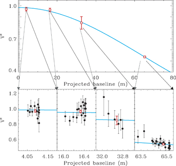
The top panel shows the baseline-averaged  measures (open circles) with the fitted uniform disc model overlaid (solid line). The bottom panels show the individual V2 measures (filled circles) at each baseline.
Formal uncertainties in θUD and A, derived from the diagonal elements of the covariance matrix, may be underestimates for three reasons: the visibility measurement errors may not strictly conform to a normal distribution, equation (1) is non-linear, and the primary calibrator is partially resolved. The effect of these factors on the model parameter uncertainties was investigated using Markov Chain Monte Carlo (MCMC) simulations. This method involves a likelihood-based random walk through parameter space, using an implementation of a Metropolis–Hastings algorithm, and yields the full marginal posterior probability density function (PDF; for an introduction to MCMC see chapter 12 of Gregory 2005). Furthermore, the current knowledge of the system can be included in the analysis by assuming an a priori distribution. For example, knowledge of the effective wavelength and calibrator angular diameter (and associated uncertainties) can be included into the uncertainty estimation of the model parameters.
Over 25 MCMC simulations were completed, each with 106 iterations, and adopting Gaussian likelihood distributions for the effective wavelength and calibrator angular diameters. The resulting PDFs for θUD produced a 1σ parameter uncertainty approximately twice as large as the formal uncertainty derived from the covariance matrix, while those for A were approximately equal. Since the simulations take into account the uncertainties in the effective wavelength and calibrator angular diameter, we adopt the standard deviations from the MCMC simulations. We believe they represent the most realistic and conservative parameter uncertainty estimates for our data set.
Final values of θUD and A are 1.063 ± 0.034 mas and 0.992 ± 0.006, respectively. The value of A, while close to unity, indicates that the measurements are affected slightly by the incoherent flux of the faint star GJ 560 B.
The work of Davis et al. (2000) can be used to correct the angular diameter for the effect of limb darkening, provided the effective temperature (Teff), surface gravity (log g) and metallicity ([Fe/H]) are known. Since roAp stars have non-standard atmospheres and Davis et al. (2000) used atlas9 atmospheric models, we investigated the limb-darkening correction within the following large region of parameter space: Teff= 7250–8500 K, log g= 4.0–4.5, [Fe/H] =−0.3 to +0.3. The limb-darkening correction of Davis et al. (2000), at an observing wavelength 696 nm, varies between 1.0344 and 1.0426 and is more sensitive to changes in Teff than in log g or [Fe/H]. We conservatively set an uncertainty of 0.010 in the limb-darkening correction, but note that this uncertainty is small compared to the uniform disc angular diameter uncertainty.
For the fundamental parameters found in Section 5, we get a limb-darkening correction of 1.039 ± 0.010, to obtain the limb-darkened (LD) angular diameter of θLD= 1.105 ± 0.037 mas.
4 THE BOLOMETRIC FLUX OF α Cir
We derived the bolometric flux of α Cir using two different data sets. The first value was obtained by combining the observed ultraviolet flux retrieved from IUE Newly Extracted Spectra (INES) data archive, with the theoretical flux obtained from a Kurucz model (with idl routine KURGET1). To compute the integrated fluxes, we followed the same method as North (1981). The IUE measurements were used to compute the flux in the wavelength interval 1150 < λ < 3207 Å, while the flux from λ= 3210 Å to infinity was computed from the Kurucz model that best fitted the seven intrinsic colours of the star in the Geneva photometric system, retrieved from the catalogue of Rufener (1989). Moreover, the energy distribution was extrapolated to the interval 912 < λ < 1150 Å, assuming zero flux at λ= 912 Å. The resulting integrated flux was fbol= (1.28 ± 0.02) × 10−6erg cm−2 s−1, where the quoted uncertainty range corresponds to the difference between the maximum and minimum integrated fluxes allowed by the uncertainties in the parameters of the Kurucz model adopted, which, in turn, reflect the uncertainties in the photometric data.
The abnormal flux distributions that are characteristic of Ap stars make determinations such as that described above, based on atmospheric models appropriate to normal stars, rather unreliable. When spectra calibrated in flux are also available for visible wavelengths, a more reliable determination of the bolometric flux can in principle be obtained. Unfortunately, even though two low-resolution spectra calibrated in flux are available in the literature for α Cir (see catalogues by Burnashev 1985; Alekseeva et al. 1996), the errors associated with the calibrations in flux as function of wavelength are not given in the corresponding bibliographic sources. Nevertheless, we have calculated a second value for the bolometric flux using the same method as above, but replacing the synthetic spectra obtained for the Kurucz model by the two low-resolution spectra of α Cir, calibrated in flux, retrieved from the catalogues mentioned above. In this case, the flux as function of wavelength was obtained by combining the IUE measurements in the wavelength interval 1150 < λ < 3349 Å, the mean of the two low-resolution spectra calibrated in flux in the interval 3200 < λ < 7350 Å, and the flux derived from the mean of the two Kurucz models that best fitted each of the two low-resolution spectra, for wavelengths longer than 7370 Å. The integrated flux obtained in this way was fbol= (1.18 ± 0.01) × 10−6erg cm−2 s−1, where the uncertainties reflect the difference between the integrated fluxes derived when each of the two low-resolution spectra (and corresponding best-fitting Kurucz model at higher wavelengths) were considered separately.
Since the details and associated uncertainties of the calibrations in flux of the low-resolution spectra used in the latter calculation are unknown, we will take a conservative approach and allow the bolometric flux to vary within the two extremes of the values derived through the two different approaches. Hence, in what follows, we use for the bolometric flux, the mean value fbol= (1.23 ± 0.07) × 10−6erg cm−2 s−1.
5 FUNDAMENTAL PARAMETERS OF α Cir

Physical parameters of α Cir. All parameters are from the current study except the Hipparcos parallax (van Leeuwen 2007).
| Parameter | Value | Uncertainty (per cent) |
| θLD (mas) | 1.105 ± 0.037 | 3.4 |
| f bol(10−9Wm−2) | 1.23 ± 0.07 | 5.7 |
| πp (mas) | 60.36 ± 0.14 | 0.2 |
| T eff (K) | 7420 ± 170 | 2.3 |
| R (R⊙) | 1.967 ± 0.066 | 3.4 |
| L (L⊙) | 10.51 ± 0.60 | 5.7 |
| M (M⊙) | 1.7 ± 0.2 | 12 |
| Parameter | Value | Uncertainty (per cent) |
| θLD (mas) | 1.105 ± 0.037 | 3.4 |
| f bol(10−9Wm−2) | 1.23 ± 0.07 | 5.7 |
| πp (mas) | 60.36 ± 0.14 | 0.2 |
| T eff (K) | 7420 ± 170 | 2.3 |
| R (R⊙) | 1.967 ± 0.066 | 3.4 |
| L (L⊙) | 10.51 ± 0.60 | 5.7 |
| M (M⊙) | 1.7 ± 0.2 | 12 |
In Fig. 2 we show the location of α Cir in the Hertzsprung–Russell diagram. The 1σ error box and diagonal lines are based on the fundamental parameters and associated errors derived in this study (see Table 3). Three CESAM (Morel 1997) evolutionary tracks crossing the error box for α Cir are also shown. The tracks were calculated for solar metallicity using a mixing length parameter of α= 1.6. Diffusion and rotation were not included. Note that changes in the model input parameters can significantly modify the evolutionary tracks for models with the same mass. In a study of the roAp star HR 1217, Cunha, Fernandes & Monteiro (2003) found that, while changes in the mixing length parameter and convective overshoot had a minor impact on the mass derived from model fitting of the classical observables, the uncertainties in the initial helium abundance and in the global metallicity of the star resulted in a significant uncertainty in the mass determination that in the worst case could be as large as 10 per cent. Therefore, from Fig. 2 and the results of Cunha et al. (2003), we conservatively estimate the mass of α Cir to be M= 1.7 ± 0.2 M⊙. Even so, we obtain an accurate surface gravity of log g= 4.09 ± 0.08. This is a consequence of the accurately measured interferometric radius.
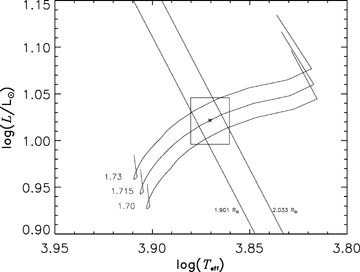
The position of α Cir in the Hertzsprung–Russell diagram, with three evolution tracks for models with masses of 1.70, 1.715 and 1.73 M⊙ for comparison. The constraints on the fundamental parameters are indicated by the 1σ error box (Teff, L/L⊙) and the diagonal lines (radius).
5.1 Comparison with previous estimates
Previous studies of α Cir have used either spectroscopy or photometric indices to estimate the fundamental atmospheric parameters. We list some recent estimates from the literature in Table 4. Kurtz & Martinez (1993) and Matthews et al. (1999) used the Strömgren Hβ index to estimate Teff. North, Berthet & Lanz (1994) made an abundance analysis of α Cir based on a few selected wavelength regions with high resolution, but the fundamental parameters were fixed based on Geneva photometry. Kupka et al. (1996) analysed high-resolution spectra of α Cir and estimated the fundamental parameters using Geneva and Strömgren photometric indices, the Balmer lines and a detailed classical analysis of several iron-peak lines. Sokolov (1998) proposed a new method to estimate Teff of roAp stars based on the slope of the continuum near the Balmer jump and found a high Teff for α Cir. Kochukhov & Bagnulo (2006) analysed a large sample of magnetic chemically peculiar stars and they used Geneva indices to estimate the fundamental parameters of α Cir. Some of the studies mentioned here that used photometric indices have not given uncertainties on the parameters. Realistic values are about 200 K, 0.2 and 0.1 dex on Teff, log g and [Fe/H], respectively (Kupka & Bruntt 2001). Kochukhov et al. (2005) explored the influence of magnetic fields on the photometric indices and found relatively small corrections, especially for field strengths of a few kG or less, as found in α Cir (see Section 6.1).
Previous estimates of log g lie in the range from 4.1 to 4.6, considering 1σ error bars. We have obtained an accurate estimate, log g = 4.09 ± 0.08, which is lower than previous estimates but in general agreement. The range in Teff estimated for α Cir in the literature is 7470–8730 K, considering 1σ error bars. This has hampered detailed studies of α Cir that rely on theoretical models, such as spectroscopic analysis (atmospheric models) or asteroseismology (evolution and pulsation models). In general the Geneva colours give lower Teff than the Strömgren or Hβ indices. The slight differences in the parameters found using the same photometric system are due to different calibrations being used. Our value, Teff= 7420 ± 170 K, is the lowest of all temperature determinations. However, it is in acceptable agreement with the Teff from Geneva indices (the mean value from four estimates is 7810 ± 160 K), and barely agrees with Teff= 7900 ± 200 K found by Kupka et al. (1996) based on spectroscopic analysis of Fe i and Fe ii lines. We note that a higher Teff is also implied in our analysis (in Section 6) of Fe i spectral lines due to a strong correlation with excitation potential. This could either imply stratification of Fe, as seen in other roAp stars, or, alternatively, that Teff of the atmospheric model is too low by 600 K. We believe the higher Teff found by Kupka et al. (1996) is explained by this.
We stress that our estimates of log g and Teff are largely model independent, unlike the previous estimates. Therefore we recommend that these values be used in future studies of α Cir. Our value for Teff depends on the angular diameter from interferometry and the bolometric flux. The latter estimate should be confirmed by making new observations.
6 SPECTRAL ANALYSIS OF α Cir
We have obtained high-quality spectra of α Cir with the Ultraviolet and Visual Echelle Spectrograph (UVES) on the Very Large Telescope. The spectra were collected as part of asteroseismic campaigns in 2004 (Kurtz et al. 2006b) and 2006. In the latter case, the spectra were used to compare the variability of α Cir in radial velocity and photometry from the star tracker on the WIRE satellite and from the ground (Bruntt et al., in preparation). The spectrum from 2004 comprises 64 co-added spectra collected over 0.5 h, at a mean rotational phase of 0.230. We define phase zero to be at minimum light in the rotational modulation curve measured with WIRE (Bruntt et al., in preparation). The spectrum from 2006 comprises 149 co-added spectra collected over 2.4 h at mean rotational phase 0.975, i.e. close to minimum light. The resulting spectra have S/N of 800 and 1100, respectively, in the continuum around 5500 Å. The spectral resolution is about R= 110 000 and we used spectra from the red arm in the wavelength ranges 4970–5950 and 6090–6900 Å. We avoided the range 5880–5950 Å, which is affected by many telluric lines. This was especially the case for the 2006 spectrum, which was collected through cloud. For this reason, we base our final results on the spectrum from 2004. The spectra were carefully normalized by identifying continuum windows in a synthetic spectrum with the same parameters as α Cir.
The spectral lines were analysed using the vwa package (Bruntt et al. 2004; Bruntt, De Cat & Aerts 2008). The abundance analysis relies on the calculation of synthetic spectra with the synth code by Valenti & Piskunov (1996). Atomic parameters and line broadening coefficients were extracted from the VALD data base (Kupka et al. 1999). Table 5 lists the lines we have used in the analysis. We used modified atlas9 models from Heiter et al. (2002) with the adopted parameters from interferometry Teff= 7420 ± 170 K and log g= 4.09 ± 0.08. We initially assumed solar metallicity, but adjusted the abundances of individual elements in the model after a few iterations. We adjusted the microturbulence to ξt= 1.60 ± 0.15 km s−1 by requiring that there is no correlation between the abundance and strength of 50 weak Fe i lines with equivalent widths <90 mÅ and excitation potentials in the range 3–5 eV. We repeated our analysis with vwa using the llmodels code (Shulyak et al. 2004), and found the same result for all elements, with differences below 0.03 dex.
The atomic number, element name, wavelength and oscillator strength (log gf) from the VALD data base for lines used in the abundance analysis. This is a sample of the full table, which is available in the online version of the article.
| Element | λ (Å) | log gf | Element | λ (Å) | log gf | Element | λ (Å) | log gf | Element | λ (Å) | log gf | Element | λ (Å) | log gf |
| 6C i | 5017.090 | −2.500 | Ti ii | 5490.690 | −2.650 | Fe i | 5217.389 | −1.070 | Fe i | 5859.578 | −0.398 | Co i | 5287.782 | −0.381 |
| C i | 5540.751 | −2.376 | 23V i | 5670.853 | −0.420 | Fe i | 5232.940 | −0.058 | Fe i | 5862.353 | −0.058 | Co i | 5342.695 | +0.690 |
| C i | 5603.724 | −2.418 | V i | 6081.441 | −0.579 | Fe i | 5242.491 | −0.967 | Fe i | 5927.789 | −1.090 | Co i | 5343.378 | −0.263 |
| C i | 5643.368 | −2.670 | V i | 6199.197 | −1.300 | Fe i | 5250.646 | −2.181 | Fe i | 5934.655 | −1.170 | Co i | 5344.560 | +0.097 |
| C i | 5800.602 | −2.338 | 24Cr i | 5204.506 | −0.208 | Fe i | 5253.462 | −1.573 | Fe i | 6056.005 | −0.460 | Co i | 5347.494 | −0.160 |
| C i | 6413.547 | −2.001 | Cr i | 5224.972 | −0.096 | Fe i | 5263.306 | −0.879 | Fe i | 6065.482 | −1.530 | Co i | 5352.045 | +0.060 |
| 8O i | 5330.737 | −0.984 | Cr i | 5247.566 | −1.640 | Fe i | 5269.537 | −1.321 | Fe i | 6078.491 | −0.424 | Co i | 5359.192 | +0.340 |
| O i | 6155.986 | −1.120 | Cr i | 5296.691 | −1.400 | Fe i | 5281.790 | −0.834 | Fe i | 6127.907 | −1.399 | Co i | 5381.768 | −0.032 |
| O i | 6156.776 | −0.694 | Cr i | 5297.376 | +0.167 | Fe i | 5283.621 | −0.432 | Fe i | 6136.615 | −1.400 | Co i | 5454.572 | −0.238 |
| O i | 6158.186 | −0.409 | Cr i | 5348.312 | −1.290 | Fe i | 5288.525 | −1.508 | Fe i | 6137.692 | −1.403 | Co i | 5483.344 | −1.490 |
The abundances relative to the Sun for 23 species2 are given in Table 6. To estimate uncertainties in the abundances we measured abundances for model atmospheres with higher values of Teff (+300 K), log g (+0.3 dex) and microturbulence (+0.4 km s−1), and made a linear interpolation using the uncertainties of these parameters. In addition, we added  to the uncertainty, where N is the number of lines, and 0.17 is the average rms standard deviation on the abundances for four elements with the most spectral lines, i.e. Ca, Fe, Co and Nd. For example, for Fe i the estimated uncertainty on the abundance is 0.08 dex, including contributions from the uncertainty on the fundamental parameters.
Abundance of α Cir relative to the Sun based on the analysis of the spectrum from 2004. The mean abundance and the number of neutral and ionized lines are denoted I and II.
| Element | [A]I | N I | [A]II | N II |
| C | +0.05 ± 0.07 | 6 | ||
| O | −0.15 ± 0.09 | 4 | ||
| Na | −0.21 ± 0.14 | 2 | ||
| Mg | −0.01 ± 0.17 | 2 | ||
| Al | +0.18 ± 0.19 | 2 | ||
| Si | −0.14 ± 0.20 | 7 | ||
| S | +0.35 ± 0.08 | 5 | ||
| Ca | +0.19 ± 0.10 | 20 | ||
| Sc | −0.42 ± 0.11 | 3 | ||
| Ti | −0.20 ± 0.13 | 5 | −0.17 ± 0.09 | 5 |
| V | +0.60 ± 0.21 | 3 | ||
| Cr | +0.48 ± 0.11 | 8 | +0.49 ± 0.10 | 11 |
| Mn | +0.68 ± 0.14 | 7 | +0.68 ± 0.09 | 4 |
| Fe | −0.12 ± 0.08 | 125 | −0.03 ± 0.05 | 20 |
| Co | +1.20 ± 0.08 | 21 | ||
| Ni | −0.58 ± 0.10 | 7 | ||
| Cu | −1.02 ± 0.18 | 2 | ||
| Y | +0.88 ± 0.12 | 10 | ||
| Zr | +0.37 ± 0.23 | 1 | ||
| Ba | −0.70 ± 0.18 | 2 | ||
| Ce | +0.74 ± 0.13 | 3 | ||
| Nda | +1.03 ± 0.10 | 12 | ||
| Eu | +1.58 ± 0.15 | 2 |
aFrom three Nd iii lines we find [Nd]=+2.06 ± 0.12.
The Fe i lines are the most numerous in the observed spectra. We find a significantly lower abundance from Fe i lines with low excitation potential, ε. For lines with 1 < ε(eV) < 3 the abundance relative to the Sun is −0.33 ± 0.02 (28 lines) and for 3 < ε(eV) < 5 the abundance is −0.07 ± 0.02 (89 lines). The quoted uncertainties are the rms on the mean value, and represent only the internal error. The difference between low and high excitation lines is significant and could be an indication of vertical stratification, meaning the abundance of Fe is higher in the deeper layers, as discussed by Ryabchikova et al. (2002, 2007).
In Fig. 3 we show a small region of the observed spectra from 2004 (solid thick line) and 2006 (dashed thick line), with identification of the elements causing the lines. We show two synthetic spectra (thin lines) with different abundances of cobalt and the rare earth element neodymium. In the first synthetic spectrum the abundances are solar and in the second we have adjusted the abundances of Co and Nd to fit the observed spectrum from 2004. We find overabundances of Co i and Nd ii of +1.20 ± 0.08 and +1.03 ± 0.11 using 21 and 12 lines, respectively. This is in acceptable agreement with the analysis by Kupka et al. (1996) who found +1.62 ± 0.20 and +1.24 ± 0.25, using six lines of each ion. For other ions listed in Table 6 we find general agreement with the previous detailed study by Kupka et al. (1996).
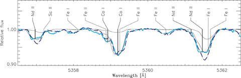
The two observed UVES spectra of α Cir are compared (solid and dashed thick lines) in a region with strong neodymium and cobalt lines. Also shown are two synthetic spectra (thin lines) for solar abundance and when the abundance of Nd and Co is increased by about a factor of 10.
The two spectra we analysed yield the same mean abundances, when averaging over several lines, with the mean abundances differing by less than 0.05–0.10 dex in the two spectra. A difference of 0.20 dex was found for V i and Eu ii, but the analysis is based on just three and two lines, respectively. It is interesting to note that the equivalent widths and detailed shapes of the Co i and Nd ii lines are significantly different in the two observed UVES spectra shown in Fig. 3. This indicates the presence of spots on the surface, as first reported by Kochukhov & Ryabchikova (2001). A more detailed study of α Cir is required to explore this, as was done for the roAp star HR 3831 by Kochukhov et al. (2004).
6.1 Limits on the magnetic field strength
The roAp stars are magnetic, with surface field strengths as high as 24.5 kG in HD 154708 (Hubrig et al. 2005), but more typically of several kG (see Kurtz et al. 2006a). Knowledge of the magnetic field strength and structure is important for the study of α Cir. A variable longitudinal magnetic field was discovered in this star by Borra & Landstreet (1975) and Wood & Campusano (1975). The latter paper shows a variable field with negative polarity and field strength extremum of −1.5 kG, but with a large uncertainty. Borra & Landstreet (1975) obtained more precise results using a photoelectric Balmer line polarimeter and could not confirm the extremum obtained by Wood & Campusano (1975). They made seven measurements over seven consecutive nights, from which they detected a variable field ranging from −560 to +420 G. From these observations they proposed a rotation period of the order of 12 d – a value we now know to be incorrect. Mathys (1991) attempted to test the possibility of a short rotation period close to 1 d by observing the longitudinal field strength. He obtained five spectra in three nights and did not detect any magnetic field within the errors of his observations. Mathys & Hubrig (1997) presented two more longitudinal field measurements which show a negative polarity magnetic field, but their results were still below the 3σ level.
From these observations it is clear that the star does have a magnetic field and that the longitudinal component is rather weak. The precision of the published observations is insufficient, however, to prove variability with the known rotation period of Prot= 4.46 d (Kurtz et al. 1994; Bruntt et al., in preparation). Bychkov, Bychkova & Madej (2005), for example, combined the data and derived a magnetic variation period equal to the known rotation period, but we conservatively are not convinced that rotational magnetic variability has been found, given the error bars of the individual measurements. While there is an indication of a rotational magnetic curve, additional high-precision observations of the longitudinal magnetic field for this bright star are sorely needed.
Estimating the magnetic field modulus 〈H〉 for α Cir is also not a simple task, given its weak longitudinal field and rather high (for an roAp star) rotational velocity of v sin i= 13 km s−1. No Zeeman components can be seen directly in our high-resolution spectra, so we searched for the effect of magnetic broadening by measuring the FWHM for selected unblended spectral lines with a spread of Landé factors. This gives a value of the magnetic field similar to the mean magnetic field modulus obtained from split Zeeman components in slowly rotating stars where the components are resolved. From the measurement of the FWHM for 20 Fe and Cr lines we obtained a magnetic field modulus of 0.9 ± 0.5 kG, a significant improvement on the upper limit of 3–3.5 kG set by Kupka et al. (1996), using a similar approach.
We estimated an upper limit for 〈H〉 by comparing average observed spectral lines with calculated lines in the presence of a magnetic field using the synthmag code (Piskunov 1999). The line of Cr ii 5116 Å with a large Landé factor of g= 2.92 is rather weak and asymmetric with a stronger blue part of the profile in the first observing set of 2004 and with a stronger red part for the second observing set from 2006. The synthetic line profile fit to this line using synthmag needed no magnetic field strength greater than 1–1.5 kG. Line profiles with large Landé factors belonging to iron, such as Fe i at 5501, 5507 and 6337 Å, fitted slightly better for a magnetic field strength up to 2 kG, in comparison with synthetic spectra with zero magnetic field. We therefore place an upper limit of 〈H〉 < 2 kG.
Romanyuk (2004) compared longitudinal magnetic field extrema with the mean magnetic field modulus for 39 Ap stars and found a linear relation: 〈H〉= 1.01 + 3.16〈Hl〉 kG. Using this relation and the extremum of the longitudinal field measurements obtained by Borra & Landstreet (1975) and Mathys & Hubrig (1997) gives a mean magnetic field modulus of 1.8 and 1.3 kG, respectively. These values are consistent with the upper limit estimated from our UVES spectra.
6.2 Simplifications: magnetic fields and NLTE
All atmospheric models include simplifications to the physical conditions in real atmospheres. This is especially the case for the roAp stars, in which magnetic fields may alter the atmospheric structure (Kochukhov et al. 2005) and where observational evidence for stratification of certain elements is found (Ryabchikova et al. 2002). More realistic models of magnetic stars are being developed (Kochukhov et al. 2005), but they indicate that the structure in α Cir should only be mildly affected by the relatively weak magnetic field of ≤2 kG that we determined above.
The atlas9 models we applied assume local thermodynamical equilibrium (LTE), but at Teff above 7000 K non-LTE (NLTE) effects become important. For a normal star with solar metallicity and Teff= 7500 K, the correction for neutral iron is [Fe i/H]NLTE= [Fe i/H]LTE+ 0.1 dex (Rentzsch-Holm 1996). This seems to agree with the slight difference in Fe abundance we find from neutral and ionized lines. We adopt this correction for our final result for the photospheric metallicity, which is the mean of the 125 Fe i lines in α Cir and, hence, [Fe/H]=−0.12 ± 0.08. We note that the overall metallicity of α Cir, below its photosphere, is much more uncertain.
7 CONCLUSION
We present the first angular diameter measurement of an roAp star, α Cir, based on interferometric measurements with SUSI. In combination with our estimate for the bolometric flux and the new Hipparcos parallax, we have determined the stellar radius and effective temperature nearly independent of theoretical atmospheric models. The constraints found in this work on the luminosity, Teff and radius will be invaluable for critically testing theoretical pulsation models of α Cir. We will present this in our companion paper, where we report the detection of the large frequency spacing in α Cir, based on photometry from the WIRE satellite (Bruntt et al., in preparation).
We analysed high-resolution spectra taken at two different rotational phases. The detailed abundance analyses yield the same mean abundances for the two spectra, but differences in the line shapes of certain elements give evidence for spots on the surface of α Cir. We confirm the abundance pattern seen in α Cir in an earlier study using fewer lines (Kupka et al. 1996). The results follow the general trend in other roAp stars, i.e. high photospheric abundance of Cr, Co, Y and the rare earth elements Nd and Eu.
Poveda et al. (1994) list the magnitude V= 8.47, while Gould & Chanamé (2004) list V= 9.46 and a separation from α Cir of 15.7 arcsec.
We quote the abundance of an ion A as [A]= log NA/Ntot− (log NA/Ntot)⊙, where N is the number of atoms and the solar values are taken from Grevesse, Asplund & Sauval (2007).
This research has been jointly funded by the University of Sydney and the Australian Research Council as part of the SUSI project. We acknowledge the support provided by a University of Sydney Postgraduate Award (APJ) and Denison Postgraduate Awards (APJ and SMO). VGE and DWK acknowledge support from the UK STFC. MC is supported by the European Community's FP6, FCT and FEDER (POCI2010) through the HELAS international collaboration and through the projects POCI/CTE-AST/57610/2004 and PTDC/CTE-AST/66181/2006 FCT-Portugal. This research has made use of the SIMBAD data base, operated at CDS, Strasbourg, France. We made use of atomic data compiled in the VALD data base (Kupka et al. 1999). We thank Christian Stütz for supplying the llmodels (Shulyak et al. 2004) we used in the analysis. We wish to thank Brendon Brewer for his assistance with the theory and practicalities of MCMC simulations.
REFERENCES
SUPPLEMENTARY MATERIAL
The following supplementary material is available for this article.
This material is available as part of the online paper from: http://www.blackwell-synergy.com/doi/abs/10.1111/j.1365-2966.2008.13167.x (this link will take you to the article abstract).
Please note: Blackwell Publishing are not responsible for the content or functionality of any supplementary materials supplied by the authors. Any queries (other than missing material) should be directed to the corresponding author for the article.
Author notes
Based on observations with the Sydney University Stellar Interferometer at the Paul Wild Observatory, Narrabri (Australia) and observations collected at the European Southern Observatory, Paranal (Chile), as part of programmes 072.D-0138 and 077.D-0150.
