


Abstract
We present the SWIRE Photometric Redshift Catalogue 1 025 119 redshifts of unprecedented reliability and of accuracy comparable with or better than previous work. Our methodology is based on fixed galaxy and quasi-stellar object templates applied to data at 0.36–4.5 μm, and on a set of four infrared emission templates fitted to infrared excess data at 3.6–170 μm. The galaxy templates are initially empirical, but are given greater physical validity by fitting star formation histories to them, which also allows us to estimate stellar masses. The code involves two passes through the data, to try to optimize recognition of active galactic nucleus (AGN) dust tori. A few carefully justified priors are used and are the key to supression of outliers. Extinction, AV, is allowed as a free parameter. The full reduced χ2ν (z) distribution is given for each source, so the full error distribution can be used, and aliases investigated.
We use a set of 5982 spectroscopic redshifts, taken from the literature and from our own spectroscopic surveys, to analyse the performance of our method as a function of the number of photometric bands used in the solution and the reduced χ2ν. For seven photometric bands (5 optical + 3.6, 4.5 μm), the rms value of (zphot−zspec)/(1 +zspec) is 3.5 per cent, and the percentage of catastrophic outliers [defined as >15 per cent error in (1 +z)], is ∼1 per cent. These rms values are comparable with the best achieved in other studies, and the outlier fraction is significantly better. The inclusion of the 3.6- and 4.5-μm IRAC bands is crucial in supression of outliers.
We discuss the redshift distributions at 3.6 and 24 μm. In individual fields, structure in the redshift distribution corresponds to clusters which can be seen in the spectroscopic redshift distribution, so the photometric redshifts are a powerful tool for large-scale structure studies. 10 per cent of sources in the SWIRE photometric redshift catalogue have z > 2, and 4 per cent have z > 3, so this catalogue is a huge resource for high-redshift galaxies.
A key parameter for understanding the evolutionary status of infrared galaxies is Lir/Lopt. For cirrus galaxies this is a measure of the mean extinction in the interstellar medium of the galaxy. There is a population of ultraluminous galaxies with cool dust and we have shown SEDs for some of the reliable examples. For starbursts, we estimate the specific star formation rate, φ*/M*. Although the very highest values of this ratio tend to be associated with Arp220 starbursts, by no means all ultraluminous galaxies are. We discuss an interesting population of galaxies with elliptical-like spectral energy distributions in the optical and luminous starbursts in the infrared.
For dust tori around type 1 AGN, Ltor/Lopt is a measure of the torus covering factor and we deduce a mean covering factor of 40 per cent.
Our infrared templates also allow us to estimate dust masses for all galaxies with an infrared excess.
1 INTRODUCTION
The ideal data-set for studying the large-scale structure of the universe and the evolution and star formation history of galaxies is a large-area spectroscopic redshift survey. The advent of the Hubble Deep Field, the first of a series of deep extragalactic surveys with deep multiband photometry but no possibility of determining spectroscopic redshifts for all the objects in the survey, has led to an explosion of interest in photometric redshifts (Gwynn & Hartwick 1996; Lanzetta, Yahil & Fernandez-Soto 1996; Mobasher et al. 1996; Sawicki, Lin & Yee 1997; Mobasher & Mazzei 1998; Arnouts et al. 1999; Fernandez-Soto, Lanzetta & Yahil 1999; Benitez 2000; Bolzonella, Miralles & Pello 2000; Fontana et al. 2000; Teplitz et al. 2001; Thompson, Weymann & Storrie-Lombardi 2001; Fernandez-Soto et al. 2002; Firth et al. 2002; Lanzetta et al. 2002; Le Borgne & Rocca-Volmerange 2002; Chen & Lanzetta 2003; Firth et al. 2003; Rowan-Robinson 2003a; Babbedge et al. 2004; Vanzella et al. 2004; Benitez et al. 2004; Collister & Lahav 2004; Gabasch et al. 2004; Mobasher et al. 2004; Rowan-Robinson et al. 2004, 2005; Wolf et al. 2004; Hsieh et al. 2005; Brodwin et al. 2006; Ilbert et al. 2006; Polletta et al. 2007). Large planned photometric surveys, both space and ground based, make these methods of even greater interest.
Here we apply the template-fitting method of Rowan-Robinson (2003a), Rowan-Robinson et al. (2004, 2005), Babbedge et al. (2004), to the data from the SPITZER-SWIRE Legacy Survey (Lonsdale et al. 2003). We have been able to make significant improvements to our method. Our goal is to derive a robust method which can cope with a range of optical photometric bands, take advantage of the Spitzer IRAC bands, give good discrimination between galaxies and quasi-stellar objects (QSOs), cope with extinguished objects, and deliver accurate redshifts out to z= 3 and beyond. With this paper we supply photometric redshifts for 1 025 119 infrared-selected galaxies and quasars which we believe are of unparalleled reliability, and of accuracy at least comparable with the best of previous work.
The areas from the SWIRE Survey in which we have optical photometry and are able to derive photometric redshifts are as follows. (1) 8.72 deg2 of ELAIS-N1, in which we have five-band (U′g′r′i′Z′) photometry from the Wide Field Survey (WFS, McMahon et al. 2001; Irwin & Lewis 2001), (2) 4.84 deg2 of ELAIS-N2, in which we have five-band (U′g′r′i′Z′ photometry from the WFS, (3) 7.53 deg2 of the Lockman Hole, in which we have 3-band photometry (g′r′i′) from the SWIRE photometry programme, with U-band photometry in 1.24 deg2, (4) 4.56 deg2 in Chandra Deep Field South (CDFS), in which we have 3-band (g′r′i′) photometry from the SWIRE photometry programme, (5)6.97 deg2 of XMM-LSS, in which we have five-band (UgriZ) photometry from Pierre et al. (2007). In addition within XMM we have 10-band photometry (ugrizUBVRI) from the VVDS programme of McCracken et al. (2003), Le Févre et al. (2004) (0.79 deg2), and very deep five-band photometry (BVRi′z′) in 1.12 deg2 of the Subaru XMM Deep Survey (SXDS, Sekiguchi et al. 2005; Furusawa et al. 2008). The SWIRE data are described in Surace et al. (2004).
Apart from the use of flags denoting objects that are morphologically stellar at some points in the code (see Section 2), we make no other use of morphological information in determining galaxy types. Thus, reference to ‘ellipticals’ etc refers to classification by the optical spectral energy distribution (SED).
A cosmological model with Λ= 0.7, h0= 0.72 has been used throughout.
2 PHOTOMETRIC REDSHIFT METHOD
In this paper, we have analysed the catalogues of SWIRE sources with optical associations with the ImpZ code [Rowan-Robinson 2003a (hereafter RR03), Rowan-Robinson et al. 2004, 2005; Babbedge et al. 2004, (hereafter B04)] which uses a small set of optical templates for galaxies and active galactic nuclei (AGN). The galaxy templates were based originally on empirical SEDs by Yoshii & Takahara (1988) and Calzetti & Kinney (1992) but have been subsequently modified in Rowan-Robinson (2003a), Rowan-Robinson et al. (2004, 2005) and Babbedge et al. (2004). Here we have modified the templates further (section 3), taking account of the large VVDS sample with spectroscopic redshifts and good multiband photometry.
The other main changes we have made to the code described by Rowan-Robinson (2003a) and Babbedge et al. (2004) are as follows.
The code involves two passes through the data. In the first pass we use six galaxy templates and three AGN templates (see section 3) and each source selects the best solution from these 9 templates. The redshift resolution is 0.01 in log10(1 +z). Quasar templates are permitted only if the source is flagged as morphologically stellar. 3.6- and 4.5-μm data are only used in the solution if log10[S(3.6)/Sr] < 0.5: this is to avoid distortion of the solution by contributions from AGN dust tori in the 3.6- and 4.5-μm bands. Longer wavelength Spitzer bands are not used in the optical template fitting.
Before commencing the solution we create a colour table for all the galaxy and QSO templates, for each of the photometric bands required, for 0.002 bins in log10(1 +z), from 0–0.85 (z= 0–6). This involves a full integration over the profile of each filter, and calculation of the effects of intergalactic absorption, for each template and redshift bin, as described in Babbedge et al. (2004). Prior creation of a colour table saves computational time.
After pass one we fit the Spitzer bands for which there is an excess relative to the starlight or QSO solution with one of four infrared templates: cirrus, M82 starburst, Arp 220 starburst and AGN dust torus, provided there is an excess at either 8 or 24 μm (cf. Rowan-Robinson et al. 2004). 3.6- and 4.5-μm data are not used in the second pass redshift solution if the emisision at 8 μm is dominated by an AGN dust torus.
In the second pass we use a redshift resolution of 0.002 in log10(1 +z). Galaxies and quasars are treated separately and for galaxies the limit on log10[S(3.6)/Sr] for use of 3.6- and 4.5-μm data in the solution is raised to 2.5, which comfortably includes all the galaxy templates for z < 6.
In pass 2, we use two elliptical galaxy templates, one corresponding to an old (12 Gyr) stellar population (which is also used in the first pass) and one corresponding to a much more recent (1 Gyr) starburst (Maraston 2005). For z > 2.5 we permit only the latter template.
In pass 2, we interpolate between the 5 spiral and starburst templates to yield a total of 11 such templates. Finer interpolation between the templates did not improve the solution.
Extinction up to AV= 1.0 is permitted for galaxies of type Sbc and later, ie no extinction for Sab galaxies or ellipticals. For quasars the limit on the permitted extinction is AV= 0.3, unless the condition S(5.8) > 1.2 S(3.6) is satisfied, in which case we allow extinction up to AV= 1.0. This condition is a good selector of objects with strong AGN dust tori (Lacy et al. 2004). If we allow AV up to 1.0 for all QSO fits, then we find serious aliasing with low redshift galaxies. The assumptions made here allow the identification of a small class of heavily reddened QSOs which is clearly of some interest. A few galaxies and quasars might find a better fit to their SEDs with AV > 1 but we found that allowing this possibility resulted in a significant increase in aliasing and a degradation of the overall quality of the redshift fits. A separate search will be needed to identify such objects.
As in Rowan-Robinson et al. (2004), a prior assumption of a power-law distribution function of AV is introduced by adding 1.5 AV to χ2ν. This avoids an excessive number of large values of AV being selected.
For galaxies, we used a standard Galactic extinction. For QSOs, we used an Large Magellanic Cloud type extinction, following Richards et al. (2003).
As in our previous work there is an important prior on the range of absolute B magnitude, essentially corresponding, for galaxies, to a range in stellar mass. Because there is strong evolution in the mass-to-light ratio (M/L) between z= 0 and 2.5, the MB limit needs to evolve with redshift. We have assumed an upper luminosity limit for galaxies of MB=−22.5 −z for z < 2.5, =−25.0 for z > 2.5, and a lower limit of MB=−17.0 −z for z < 2.5, =−19.5 for z > 2.5. For quasars we assume the upper and lower limits on luminosity correspond to MB=−26.7 and −18.7 (see Section 4 and Fig. 2 for a justification of these assumptions). We do not make any prior assumption about the shape of the luminosity function. Strictly speaking, it would be better to limit the near infrared luminosity to constrain the range of stellar mass, but we found that by specifying a limited range of MB we were also eliminating unreasonably large star formation rates in late-type galaxies.
We have accepted the argument of Ilbert et al. (2006) that it is necessary to apply a multiplicative in-band correction factor to each band to take account of incorrect photometry and calibration factors. Table 1 gives these factors for each of our areas, determined from samples with spectroscopic redshifts.
In calculating the reduced χ2ν for the redshift solution we use the quoted photometric uncertainties, but we set a floor to the error in each band, typically 0.03 magnitudes for g, r, i, 0.05 mag for u, z, 1.5 μJy for 3.6 μm and 2.0 μJy for 4.5 μm.
This also implies a maximum weight given to any band in the solution. Without this assumption, there would be cases where a band attracted unreasonably high weight because of a spuriously low estimate of the photometric error.
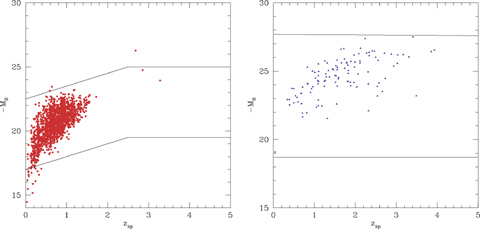
Left-hand panel: absolute blue magnitude, MB, versus spectroscopic redshift for galaxies in SWIRE-VVDS (L) and QSOs in SWIRE-Lockman (R).
Correction factors for fluxes in each band, by area.
| Area | U′ | g′ | r′ | i′ | Z′ | J | H | K | 3.6 μm | 4.5 μm |
| EN1,EN2 | 1.114 | 0.988 | 0.951 | 0.994 | 1.004 | 1.238 | 1.171 | 1.130 | 0.954 | 0.993 |
| Lockman | 1.057 | 1.031 | 0.901 | 0.910 | 1.050 | 1.002 | ||||
| VVDS | 1.046 | 0.969 | 0.928 | 0.960 | 0.972 | 1.173 | 1.029 | 1.085 | 1.015 | |
| XMM-LSS | 1.046 | 0.969 | 0.928 | 0.960 | 0.972 | 1.085 | 1.015 | |||
| CDFS | 1.046 | 0.969 | 0.916 | 0.991 | 0.972 | 1.045 | 1.037 |
We have not used some of the other priors used by Ilbert et al. (2006), for example use of prior information about the redshift distribution, nor their very detailed interpolation between templates. We have found that while carefully chosen priors are essential to eliminate aliases, which are the main cause of outliers, it is also crucial to keep the code as simple as possible since unnecessary complexity creates new outliers.
Aperture matching between bands is a crucial issue for photometric redshifts and we have proceeded as follows. At optical wavelengths we use colours determined in a point-source aperture, but then apply an aperture correction to all bands defined in the r band by the difference between the Sextractor mag-auto and the point-source magnitude. For the IRAC bands, we use ‘ap-2’ magnitudes, corresponding to a 1.9-arcsec-radius aperture, except that if the the source is clearly extended, defined by Area (3.6) > 250, we use Kron magnitudes. For the 2MASS J, H, K magnitudes, we use the extended source catalogue magnitude in a 10-arcsec aperture, if available, and the point-source catalogue magnitude otherwise. For 80 per cent of sources with 2MASS associations, the JHK magnitudes improve the fit slightly, but for 20 per cent the addition of the JHK magnitudes makes the χ2 for the solution significantly worse. We found the same problem for associations with the UKIDSS DXS survey in EN1, with the corresponding proportions being 70:30. The issue is almost certainly one of aperture matching. We have not included JHK data in the analysis of the performance of the photometric redshift method given here.
The requirement for entry to the code is that a source be detected in at least one SWIRE band and in at least one optical band out of gri. We are then able to determine redshifts for ∼95 per cent of sources, except in EN1, where the figure drops to 85 per cent. The additional failure rate n EN1 is primarily due to photometry in one of the optical bands being out of line with the other bands. Other reasons for failure can be that after imposing 3σ limits on all bands, there are no longer two bands available out of UgriZ, 3.6, 4.5 μm. Of course redshifts determined from only two photometric bands are of low reliability (see Section 4.3).
3 TEMPLATES
3.1 Galaxy templates
The choice of the number and types of template to use is very important. If there are too few templates, populations of real sources will not be represented, whilst if there are too many there will be too much opportunity for aliases and degeneracy.
The ImpZ code uses six galaxy templates (RR03, B04 and Babbedge et al. 2006); E, Sab, Sbc, Scd, Sdm and starburst galaxies. These six templates (or similar versions) have been found to provide a good general representation of observed galaxy SEDs. The original empirical templates used in RR03 were adapted from Yoshii & Takahara (1988), apart from the starburst template, which was adapted from observations by Calzetti & Kinney (1992). These templates have been subsequently modified, as described below, to improve the photometric redshift results.
In B04 those empirical templates were regenerated to higher resolution using simple stellar populations (SSPs), each weighted by a different SFR and extinguished by a different amount of dust, AV. This procedure, based on the synthesis code of Poggianti (2001), gave the templates a physical validity. Minimization was based on the Adaptive Simulated Annealing algorithm. Details on this algorithm and on the fitting technique are given in Berta et al. (2004). These templates were used by ImpZ in Babbedge et al. (2006) in order to obtain photometric redshifts and calculate luminosity functions for IRAC and MIPS sources in the ELAIS N1 field of the SWIRE survey.
We have now improved these templates further in a two stage process using the rich multi-wavelength photometry and spectroscopic redshifts in the CFH12K-VIRMOS survey (Le Févre et al. 2004): a deep BVRI imaging survey conducted with the CFH-12K camera in four fields. Additionally, there are U-band data from the 2.2-m telescope in La Silla, J and K data from the NTT and IRAC and MIPS photometry from the SWIRE survey. The spectroscopic redshifts come from the follow-up VIRMOS-VLT Deep Survey (VVDS: Le Févre et al. 2003), a large spectroscopic follow-up survey which overlaps with the SWIRE data in the XMM-LSS field.
The spectroscopic sample is sufficiently large (5976 redshifts) and wide ranging in redshift (0.01 < z < 4) to allow a detailed comparison between the template SEDs and observed SEDs. We first find the best-fitting template SED for each VVDS source with the photometric redshift set to the spectroscopic redshift (for sources with i < 22.5, nzflag = 3 or 4 (Le Févre et al. 2005; Gavignaud et al. 2006), ie reliable galaxy redshifts). We typically find ∼100–400 sources for each of the six galaxy templates (after discarding those which do not obtain a fit with reduced χ2ν < 5). A comparison of the renormalized, extinction-corrected rest-frame fluxes from each set of sources to their best-fitting galaxy template then highlights potential wavelength ranges of the template that fail to reproduce well the observed fluxes (typically from ∼1200 Å to >5 μm). This comparison is shown in Fig. 1. We then adapt those regions of the templates to follow the average track shown by the observed datapoints. These adapted templates are once again empirical and in order to recover their physical basis we then reproduce them via the same SSP method as used in B04. These final templates are then both physically based and provide a very good representation of the observed sources from the VVDS survey. For a comparison, see Fig. 1 and for details of the SSPs and their contribution to each template, see Table 2.
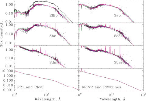
The new SED templates (red) compared with the old ones (green) and data from VVDS photometry (purple: r < 21.5, black: r > 21.5). The black SED (displaced) is the modified Maraston (2005) proto-elliptical.
The six galaxy templates and the SSPs that were used to create them. SFR is scaled to give a total mass of 1E11 M⊙.
| SSP | SED template | |||||||||||||
| # | Age (yr) | Δt (yr) | Elliptical (E1) | Sab | Sbc | Scd | Sdm | Starburst | ||||||
| SFR | E(B−V) | SFR | E(B−V) | SFR | E(B−V) | SFR | E(B−V) | SFR | E(B−V) | SFR | E(B−V) | |||
| 1 | 1 × 10⁶ | 2 × 10⁶ | – | – | – | – | – | – | – | – | – | – | 181.5 | 1.4 |
| 2 | 3 × 10⁶ | 4 × 10⁶ | – | – | – | – | – | – | – | – | – | – | 8.74 | 4.8E−6 |
| 3 | 7 × 10⁶ | 1.3 × 10⁷ | – | – | 1.71 | 0.11 | 8.7 | 0.17 | 53.4 | 0.77 | 47.6 | 0.079 | – | – |
| 4 | 8 × 10⁶ | 3 × 10⁶ | – | – | – | – | – | – | – | – | – | – | 1.2E−3 | 4.8E−6 |
| 5 | 1 × 10⁷ | 4 × 10⁶ | – | – | – | – | – | – | – | – | – | – | 3.2E−4 | 4.8E−6 |
| 6 | 5 × 10⁷ | 6.2 × 10⁷ | – | – | – | – | – | – | – | – | – | – | 2.9E−4 | 4.8E−6 |
| 7 | 9 × 10⁷ | 1.87 × 10⁸ | – | – | 3.1E−3 | 0.11 | 2.5E−3 | 0.17 | 1.12 | 0.047 | 4.6E−2 | 0.079 | – | – |
| 8 | 1 × 10⁸ | 1.25 × 10⁸ | 0.53 | 4.3E−7 | – | – | – | – | – | – | – | – | 3.4E−4 | 4.8E−6 |
| 9 | 3 × 10⁸ | 2 × 10⁸ | 1.5E−4 | 4.3E−7 | – | – | – | – | – | – | – | 45.4 | 7.7E−10 | |
| 10 | 4.5 × 10⁸ | 5.5 × 10⁸ | – | – | 2.27 | 1.8E−4 | 6.1 | 1.9E−4 | 7.15 | 0.007 | 45.5 | 8.1E−9 | – | – |
| 11 | 5 × 10⁸ | 3.5 × 10⁸ | 2.7E−3 | 4.3E−7 | – | – | – | – | – | – | – | – | 1.0E−3 | 7.7E−10 |
| 12 | 1 × 10⁹ | 1.25 × 10⁹ | 3.38 | 3.3E−8 | 1.3E−3 | 1.8E−4 | 2.7E−5 | 1.9E−4 | 7.9E−3 | 0.0071 | – | – | 2.6E−5 | 7.7E−10 |
| 13 | 2 × 10⁹ | 1 × 10⁹ | 1.5E−3 | 3.3E−8 | 4.6E−3 | 1.8E−4 | 1.2E−4 | 1.9E−4 | 8.0E−2 | 0.0071 | 2.3E−2 | 8.1E−9 | 2.0E−5 | 7.7E−10 |
| 14 | 4 × 10⁹ | 1.5 × 10⁹ | 1.1E−3 | 3.3E−8 | 6.3E−4 | 1.8E−4 | – | – | 4.0E−2 | 0.0071 | 2.2E−3 | 8.1E−9 | 9.6E−6 | 7.7E−10 |
| 15 | 7 × 10⁹ | 3 × 10⁹ | 3.0E−4 | 3.3E−8 | 5.2E−3 | 1.8E−4 | 8.9E−5 | 1.9E−4 | 6.4E−2 | 0.0071 | 9.7E−3 | 8.1E−9 | 3.8E4 | 7.7E−10 |
| 16 | 1 × 10¹⁰ | 3 × 10⁹ | 3.3E−3 | 3.3E−8 | 1.9E−4 | 1.8E−4 | 3.3E−3 | 1.9E−4 | 26.8 | 0.0071 | 2.5E−2 | 8.1E−9 | 2.9E−4 | 7.7E−10 |
| 17 | 1.2 × 10¹⁰ | 2 × 10⁹ | 47.8 | 3.3E−8 | 49.4 | 1.1E−6 | 48.3 | 2.3E−5 | 23.5 | 2.1E−4 | 44.5 | 8.1E−9 | 45.3 | 7.7E−10 |
3.1.1 Ellipticals
In addition to our standard elliptical template we now include (in the second pass) a young elliptical template. This young elliptical is based on a 1-Gyr-old SSP provided by Claudia Maraston (2005). A significant improvement for high-redshift galaxy studies is the treatment in this template of thermally pulsing the asymptotic giant branch (TP-AGB) phase of stellar evolution, particularly in the near-IR. Maraston (2006) has demonstrated that this phase has a strong contribution to the infrared SED of galaxies in the high-redshift Universe (z∼ 2). Because of the limited time for evolution available at higher redshifts, we restrict ellipticals to just this template for z > 2.5.
The Maraston elliptical template did not have a ‘ultraviolet (UV) bump’ but since we have found that our higher redshift ellipticals did exhibit some UV emission, we have replaced the template shortward of 2100 Å with the UV behaviour of our old (12 Gyr) elliptical. We are not able to say whether this UV upturn is due to a recent burst of star formation (but see section 8 for some hint that this may be relevant), to horizontal branch stars, or to binary star evolution. Additionally, as the TP-AGB stellar templates incorporated into the evolutionary population synthesis of Maraston (2006) are empirical, they do not extend longward of 3 μm, so we have followed a similar procedure as above to derive the behaviour at λ > 3 μm.
An important benefit of these stellar synthesis fits to our templates is that we can estimate stellar masses for all SWIRE galaxies (see Section 8).
3.2 AGN templates
As well as galaxy templates, the inclusion of a number of different AGN templates has been considered to allow the ImpZ code to identify quasar-type objects as well as normal galaxies. B04 tested the success of including the the SDSS median composite quasar spectrum (Vanden Berk 2001) and red AGN templates such as the z= 2.216 FIRST J013435.7−093102 source from Gregg (2002) but found that two simpler AGN templates were most useful. These were based on the mean optical quasar spectrum of Rowan-Robinson (1995), spanning 400 Å to 25 μm. For wavelengths longer than Lyα the templates are essentially αλ≈−1.5 power laws, with slight variations included to take account of observed SEDs of ELAIS AGN (Rowan-Robinson et al. 2004). Following a number of further tests and template alterations, we now make use of updated versions of these two AGN templates: AGN1 has been improved (now called RR1v2) in a similar procedure as applied in Section 3.1 using the spectroscopic dataset to indicate regions of poor agreement between the template and photometry; AGN2 (now RR2v2) has also been modified to create a third template, RR2v2lines, by adding Lyα and C iv emission lines and the whole template then adapted via comparison to photometry (as with the other templates). This means ImpZ makes use of three AGN templates, whose main difference is the presence/lack of Lyα and C iv emission, as well as the amount of flux longward of 1 μm. The numbers of quasars selecting the 3 templates are 6568 (0.65 per cent) (RR1v2), 5253 (0.52 per cent) (RR2v2) and 5853 (0.58 per cent) (RR2v2lines). Use of a template like that derived by Richards et al. (2003) from SDSS quasars, which has very strong emission lines, generated many more aliases.
4 RESULTS FROM THE IMPZ2 PHOTOMETRIC REDSHIFT CODE
4.1 Justification of priors on MB
Fig. 2 shows the absolute B magnitude versus spectroscopic redshift for galaxies and quasars. The photometric redshift code was run with z forced to be equal to the spectroscopic redshift, but other parameters (template type, extinction) allowed to vary, and MB then calculated for the best solution. The assumed limits on MB are shown and look reasonable. The limit at the low end does exclude some very low luminosity galaxies and for these the photometric redshift would be biased to slightly higher redshift. However, lowering the lower boundary results in low-redshift aliases for galaxies whose true redshift is much higher.
The increase of maximum luminosity with redshift reflects the strong evolution in mass-to-light ratio with redshift since z∼ 2. van der Wel et al. (2005) find d ln(M*/LK) ∼−1.2 z and d ln(M*/LB) ∼−1.5 z for 0 < z < 1.2 for early-type galaxies. We needed to continue this trend to redshift 2.5 to accomodate some of the z∼ 3 galaxies found by Berta et al. (in preparation), based on the IRAC ‘bump’ technique of Lonsdale et al. (2007). At higher redshifts, the maximum luminosity should decline, reflecting the accumulation of galaxies, but we have not tried to model that in detail here. The apparent increase in the maximum luminosity with redshift may also be in part due to the increasing volume being sampled as redshift increases.
4.2 Impact of number of photometric bands available
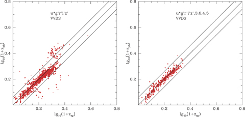
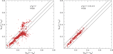
To analyse the impact of the number of optical photometric bands available, and of what improvement is afforded by being able to use the Spitzer 3.6- and 4.5-μm data, we have carried out a detailed analysis of the spectroscopic sample from the VVDS survey (Le Févre et al. 2004). Figs 3–7 show results from our code, paired so that the left-hand plot in each case is the result for optical data only, while the right-hand plots show the impact of including 3.6- and 4.5-μm data in the solution. Note that there are some additional objects on the left-hand plots which are undetected at 3.6 or 4.5 μm. Figs 3(L)–7(L) show a comparison of log10(1 +zphot) versus log10(1 +zspec) for VVDS using 10 (ugrizUBVRI), five (ugriz), four (ugri or griz) and three (gri) optical bands without using 3.6- and 4.5-μm data. Figs 3(R)–6(R) show corresponding plots when 3.6- and 4.5-μm data are used. The latter show a dramatic reduction in the number of outliers. Inclusion of 3.6- and 4.5-μm bands has a more significant effect than Increasing the number of optical bands from 5 to 10. Absence of the U band does significantly worsen performance, especially at z < 1, but with gri+ 3.6, 4.5 there is still an acceptable performance.
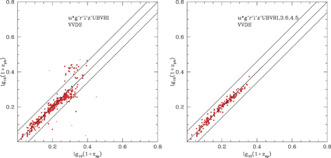
Left-hand panel: photometric versus spectroscopic redshift for SWIRE-VVDS sources, using 10 optical bands (ugrizBV RI) and requiring r < 23.5. The larger dots are those classified spectroscopically as galaxies, while the small dots are those classified spectroscopically as quasars (but our code selects a galaxy template). Right-hand panel: Photometric versus spectroscopic redshift for SWIRE-VVDS sources, using 10 optical bands (ugrizBV RI) + 3.6, 4.5 μm, and requiring r〈23.5, S(3.6)〉 7.5 μJy. The tram-lines in this and subsequent plots correspond to Δlog10(1 +z) =±0.06, that is, ±15 per cent, our boundary for catastrophic outliers.
Left-hand panel: photometric versus spectroscopic redshift for SWIRE-VVDS sources, using five optical bands only (ugriz) and requiring r < 23.5. Right-hand panel: photometric versus spectroscopic redshift for SWIRE-VVDS sources, using five optical bands (ugriz) + 3.6, 4.5 μm, and requiring r < 23.5, S(3.6) > 7.5 μJy.
Left-hand panel: photometric versus spectroscopic redshift for SWIRE-VVDS sources, using four optical bands only (ugri) and requiring r < 23.5. Right-hand panel: photometric versus spectroscopic redshift for SWIRE-VVDS sources, using four optical bands (ugri) + 3.6, 4.5 μm, and requiring r < 23.5, S(3.6) > 7.5 μJy.
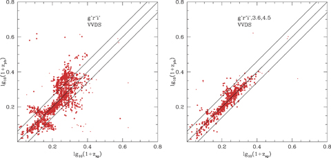
Left-hand panel: photometric versus spectroscopic redshift for SWIRE-VVDS sources, using three optical bands only (gri) and requiring r < 23.5. Right-hand panel: photometric versus spectroscopic redshift for SWIRE-VVDS sources, using three optical bands (gri) + 3.6, 4.5 μm, and requiring r < 23.5, S(3.6) > 7.5 μJy.
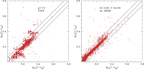
Left-hand panel: photometric versus spectroscopic redshift for SWIRE-VVDS sources, using four optical bands only (griz) and requiring r < 23.5. Right-hand panel: photometric versus spectroscopic redshift for all SWIRE sources with spectroscopic redshift, using at least four bands in total and requiring r < 23.5, S(3.6) > 7.5 μJy
Fig. 7(R) shows log10(1 +zphot) versus log10(1 +zspec) for the whole SWIRE survey requiring at least 4 bands in total, S(3.6) > 7.5 μ Jy, r < 23.5, 4 photometric bands (which could be, say, gri+ 3.6 μm) is the minimum number for reliable photometric redshifts. Fig. 8 shows the corresponding plots in the SWIRE-EN1 and SWIRE-Lockman areas, where we have carried out programs of spectroscopy (Trichas et al., in preparation; Owen & Morrison, in preparation; Berta et al. 2007), for a minimum of six photometric bands in total, and Fig. 9 shows the same plot for the whole of SWIRE, requiring a minimum of 6 photometric bands. We see that our method gives an excellent performance for galaxies out to z= 1 (and beyond). Demanding more photometric bands discriminates against high-redshift objects, which will start to drop out in short wavelength bands, and against quasars because they tend to have dust tori and therefore the 3.6- and 4.5-μm bands are not used in the solution.
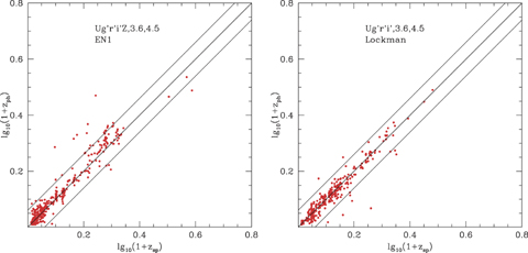
Left-hand panel: photometric versus spectroscopic redshift for SWIRE-EN1 sources (UgriZ+ 3.6, 4.5 μm), using at least 6 bands and requiring r < 23.5, S(3.6) > 7.5 μ Jy. Most of the spectroscopic redshifts at z > 0.5 are from the programme of Berta et al. (2007) and Trichas et al. (in preparation). Right-hand panel: photometric versus spectroscopic redshift for SWIRE-Lockman sources (Ugri+ 3.6, 4.5 μm), using six bands and requiring r < 23.5, S(3.6) > 7.5 μJy. Most of the spectroscopic redshifts at z > 0.5 are from the programme of Berta et al. (2007) and Smith et al. (in preparation).
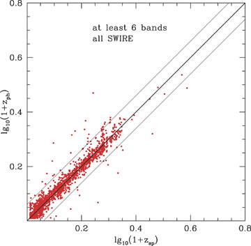
Photometric versus spectroscopic redshift for all SWIRE galaxies with spectroscopic redshifts, using at least six bands and requiring r < 23.5, S(3.6) > 7.5 μ Jy.
The performance worsens for z > 1.5, though we do not really have enough spectroscopic data to fully characterize this. For 31 galaxies with zph, detected in at least five bands, with r < 23.5, S(3.6) > 7.5 μJy, we found that nine (29 per cent) had |log10(1 +zphot) − log10(1 +zspec| > 0.15, and the rms of (zphot−zspec)/(1 +zspec) for the remainder was 11 per cent.
In EN1, there appears to be a slight systematic overestimation of the redshift around z∼ 1, by about 0.1. This is not seen in the VVDS or Lockman samples, or in the overall plot for the whole SWIRE Catalogue (Fig. 9). The most likely explanation is some bias in the WFS photometry at fainter magnitudes.
4.3 Dependence of performance on r and χ2ν
The rms deviation of (zphot−zspec)/(1 +zspec) depends on the number of photometric bands, the limiting optical magnitude, and the limiting value of χ2 (see Figs 11 and 12), but a typical value for galaxies is 4 per cent, a significant improvement on our earlier work. For comparison, typical rms values found by Rowan-Robinson (2003a) and Rowan-Robinson et al. (2004) from UgriZ, JHK data alone were 9.6 and 7 per cent, respectively.
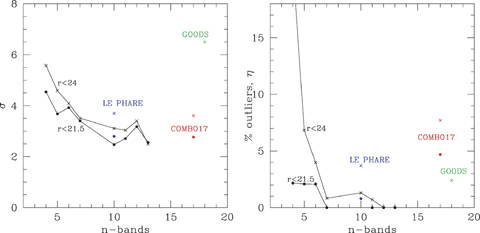
Left-hand panel: per cent rms of (zphot−zspec)/(1 +zspec), excluding outliers, versus total number of photometric bands for SWIRE sources. Figures for 10 or more bands are from the SWIRE-VVDS survey. Figures for COMBO-17 (Wolf et al. 2004) and GOODS (Mobasher et al. 2004) are also shown. Right-hand panel: η per cent outliers versus total number of photometric bands for SWIRE sources. The filled circles are values for r < 21.5, and the crosses are for r < 24.
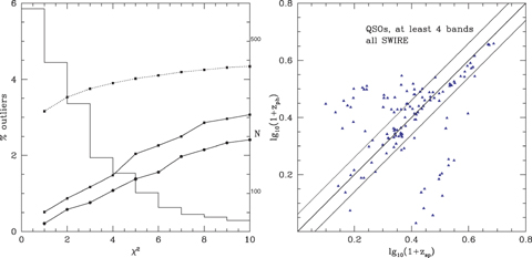
Left-hand panel: per cent rms of (zphot−zspec)/(1 +zspec) versus χ2 limit (dotted curve, left-hand scale) for SWIRE sources with at least seven photometric bands. Per cent outliers versus χ2ν limit (solid curves, left-hand scale, upper curve r < 24, lower curve r < 21.5). Also shown is a histogram of χ2ν values (right-hand scale). Right-hand panel: photometric versus spectroscopic redshift for SWIRE quasars detected in four photometric bands.
Fig. 10 shows the dependence of log10(1 +zphot)/(1 +zspec) on the r magnitude and on the value of the reduced χ2ν. The percentage of outliers stars to increase for r > 22. Although we treat χ2ν > 10 as a failure of the photometric method (due for example to poor photometry or confusion with a nearby optical object), there is still a good correlation of photometric and spectroscopic redshift.
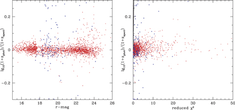
Left-hand panel: log10(1 +zphot/(1 +zspec) versus r for all SWIRE sources. Red = galaxies, blue = quasars. Right-hand panel: log10(1 +zphot/(1 +zspec) versus χ2 for all SWIRE sources.
Fig. 11 shows how the rms value of log10(1 +zphot)/(1 +zspec), σ and the percentage of outliers, η, defined as objects with |log10(1 +zphot)/(1 +zspec)| > 0.06, as a function of the total number of photometric bands. The rms values are comparable or slightly better than those of Ilbert et al. (2006) derived from the VVDS optical data using the le phare code. For seven or more bands (e.g. UgriZ+ 3.6, 4.5 μm) the rms performance is comparable to the 17-band estimates of COMBO-17 (Wolf et al. 2004), significantly better than those of Mobasher et al. (2004) with GOODS data, and comparable to Mobasher et al. (2007). The outlier performance is significantly better than Wolf et al. (2004), Ilbert et al. (2006) and Mobasher et al. (2007), which we attribute to the use of the SWIRE 3.6- and 4.5-μm bands. Fig. 12(L) show the same quantities as a function of the limit on the reduced χ2ν, together with a histogram of χ2ν values, for SWIRE sources with at least seven photometric bands. The figures for COMBO-17 data were derived from their published catalogue using exactly the same procedure as for the SWIRE data. Those for GOODS were taken from table 1 of Mobasher et al. (2004). Of course, where the number of optical bands is greater than 5, there is generally considerable overlap between the bands (typically U′griZ′ plus U BV RI), so the number of bands is not a totally fair measure of the amount of independent data being used (this applies to our analysis of the VVDS data, and to the GOODS and COMBO17 analyses).
While the rms values found in several different studies are comparable, the dramatic improvement here is in the reduction of the number of outliers, when sufficient photometric bands are available. The remaining outliers tend to be due either to bad photometry in one band or to aliases.
4.4 Performance for QSOs
The photometric estimates of redshift for AGN are more uncertain than those for galaxies, due to aliassing problems, but the code is effective at identifying type 1 AGN from the optical and near ir data. For some quasars there is significant torus dust emission in the 3.6- and 4.5-μm bands, and since the strength of this component varies from object to object, inclusion of these bands in photometric redshift determination with a fixed template can make the fit worse rather than better. We have therefore omitted the 3.6- and 4.5-μm bands if S(3.6)/S(r) > 3. Note that only 1.75 per cent of SWIRE sources are identified by the photometric redshift code as type 1 AGN, and of these only 5 per cent are found to have AV > 0.5.
Fig. 12(R) shows photometric versus spectroscopic redshift for SWIRE quasars detected in at least four photometric bands. One-third of QSOs (53/158) have |log10(1 +zphot)/log10(1 +zspec)| > 0.10 and the rms deviation for the remainder is 9.3 per cent. Many of the outliers are cases where because an almost power-law SED is being fitted, the redshift uncertainty is very wide indeed.
Redshift estimates for AGN can be affected by optical variability since optical photometry for different bands may have been taken at different epochs, as in the INT-WFS photometry in EN1 and EN2 (Afonso-Luis et al. 2004).
Richards et al. (2001) and Ball et al. (2007) have given similar estimates of rms and outlier rate for photometric redshifts for quasars. Because we are rarely able to use 3.6- and 4.5-μm data in the photometric redshift solution, we do not expect to have any advantage over fits using purely optical data. However, it is worth emphasizing that our code appears to be effective in selecting the type 1 AGN without any spectroscopic information.
5 CATALOGUE DESCRIPTION
The SWIRE Photometric Redshift Catalogue consists of 1 025 119 sources, split between the SWIRE fields as follows: EN1 (218 117), EN2 (125 364), Lockman (229 238), SWIRE-VVDS (34 630), SWIRE-SXDS (55 432), XMM (excluding VVDS and SXDS) (212 572), Chandra DFS (149 766). It is available via IRSA and also at http://astro.ic.ac.uk/~mrr/swirephotzcat.
The columns listed are:
nidir(i8), infrared identifier
nidopt(i8), optical identifier
RA(f11.6), RA in degrees
Dec.(f11.6), Dec. in degrees
s36(f10.2), S(3.6 μm) in μJy
s24(f10.2), S(24 μm) in μJy
s70(f10.2), S(70 μm) in μJy
am3(f8.2), r-band mangnitude (AB magnitudes for XMM-LSS,
Vega for all the other regions)
j1(i3), optical template type (1–11 galaxies (one E, two E′, three
Sab, five Sbc, seven Scd, nine Sdm, 11 Sb), 13–15 QSOs) for
AV= 0 solution
alz(f7.3), log10(1 +zphot) for AV= 0 solution
err0(f10.3), reduced χ2 for AV= 0 solution
j2(i3), optical template type (1–11 galaxies, 13–15 QSOs) for free
AV solution
alz2(f7.3), log10(1 +zphot) for free AV solution
av1(f6.2), AV
err1(f10.3), reduced χ2 for free AV solution
n91(i3), total number of photometric bands in solution
nbopt(i3), number of optical bands in solution
amb2(f8.2), MB (corrected for extinction) for free AV solution
alb(f8.2), log10LB, in solar units
spectz0(f10.5), spectroscopic redshift
nzref0(i4), reference for spectroscopic redshift [N1,N2: nzref0 = 1-9, as in Rowan-Robinson 2003a; = 11 Keck redshifts (Berta et al. 2007), = 20 WIYN redshifts (Trichas et al., in preparation), = 25 GMOS redshifts (Trichas et al., in preparation), = 30 (Swinbank et al. 2007); VVDS: nzref0 = 3-14 VVDS quality flag; Lockman: nzref0 =−1, 1 to 4 (Steffen et al. 2004), = 5 NED, = 10 WIYN, Keck, Gemini redshifts (Smith et al., in preparation), = 11 Keck redshifts (Berta et al. 2007); XMM, CDFS: nzref0 = 5 NED]
nir(i3), number of bands with infrared excess
alp1(f6.2), relative amplitude of cirrus component at 8 μm (s.t. alp1+alp2+alp3+alp4=1)
alp2(f6.2), relative amplitude of M82 starburst component at 8 μm
alp3(f6.2), relative amplitude of AGN dust torus component at 8 μm
alp4(f6.2), relative amplitude of A220 component at 8 μm
errir3(f10.3), reduced χ2ν of infrared template fit
alcirr(f8.2), log10Lcirr in solar units (1-1000 μm), upper limits shown −ve, assuming alp1 ≤0.05
alsb(f8.2), log10LM82 in solar units, upper limits shown −ve, assuming alp2 ≤0.05
alagn(f8.2), log10Ltor in solar units, upper limits shown −ve, assuming alp3 ≤0.05
al220(f8.2), log10LA220 in solar units, upper limits shown −ve, assuming alp4 ≤0.05
alir(f8.2), log10Lir in solar units
nirtemi3, ir template type (dominated by cirrus(1), M82 starburst(2), A220 starburst(3), AGN dust torus(4), single band excess(5), no excess(6)
als70(f6.2), log10 S70, als160(f6.2), log10 S160, als350(f6.2), log10 S350, als450(f6.2), log10 S450, als850(f6.2), log10 S850, als1250(f6.2), log10 S1250, predicted from in template fit in μJy
al36(f8.2), log10L(3.6 μ) in units of L⊙
alm(f8.2) log10M*/M⊙, stellar mass in solar units
alsfr(f8.2) log10sfr, star formation rate in M⊙ yr−1
almdust(f8.2) log10Mdust/M⊙, dust mass in solar units
chi2(85f6.2), array of reduced χ2ν as function of alz2, minimized over all templates, in bins of 0.01 in log10(1 +zph), from 0.01 to 0.85.
6 REDSHIFT DISTRIBUTIONS
Fig. 13L shows the redshift distributions derived in this way for SWIRE-SXDS sources with S(3.6) > 5 μJy, above which flux the optical identifications (to r∼ 27.5) are relatively complete, with a breakdown into elliptical, spiral + starburst and quasar SEDs based on the photometric redshift fits. Fig. 13(R) shows the corresponding histograms for the whole SWIRE catalogue. Here we have subdivided this into E, Sab, Sbc, Scd, starbursts and quasars. The latter distribution starts to cut off at slightly lower redshift, ∼1.5, because the typical depth of the optical data is r∼ 24–25 instead of 27.5.
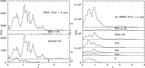
Left-hand panel: photometric redshift histogram for SWIRE-SXDS sources with six good photometric bands, and S(3.6) > 5 μJy, r < 27.5. Top panel: all sources; lower panels: separate breakdown of contributions of ellipticals, spirals (Sab + Sbc + Scd) + starbursts (Sdm + Sb), and quasars. The histogram for quasars has been multiplied by 20. Right-hand panel: photometric redshift histogram for all SWIRE sources with four good photometric bands, and S(3.6) > 5 μJy. Top panel: all sources; lower panels: separate breakdown of contributions of ellipticals, Sab, Sbc, Scd, starbursts (Sdm + Sb), and quasars. The histogram for quasars has been multiplied by 10.
A small secondary redshift peak appears for galaxies at z∼ 3. About two-thirds of these have aliases at lower redshifts and some of these z∼ 3 sources are spurious (see Fig. 7R). However, there is a real effect favouring detection of galaxies at z∼ 3, that the starlight peak at ∼1 μm entering the IRAC bands generates a negative K-correction at 3.6 and 4.5 μm. Spectroscopy is needed to ascertain the reality of this peak.
Ellipticals cut off fairly sharply at z∼ 1. At z > 2 sources tend to be starbursts or quasars. The structure seen in the redshift distribution may be partly a result of redshift aliasing, but bearing in mind the estimated accuracy of these redshifts [typically 4 per cent in (1 +z)], some of the grosser features may indicate large-scale structure within the SWIRE fields. Fig. 14(L) shows the redshift distribution in EN1, in which peaks appear at z∼ 0.3, 0.5, 0.9, 1.1. From Fig. 8L, we see that the spectroscopic redshifts show clear clusters at z= 0.31, 0.35, 0.47, 0.9 and 1.1, so the peaks in Fig. 14(L) do seem to correspond to real structure. The peak at z∼ 0.9 corresponds to the supercluster seen by Swinbank et al. (2007).
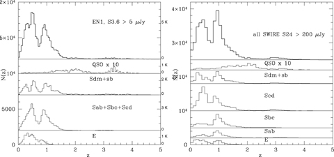
Left-hand panel: photometric redshift histogram for SWIRE-EN1 sources with at least five photometric bands, and S(3.6) > 5 μJy. Top panel: all sources; lower panels: separate breakdown of contributions of ellipticals, spirals (Sab + Sbc + Scd) + starbursts (Sdm + Sb), and quasars. The histogram for quasars has been multiplied by 20. Right-hand panel: photometric redshift histogram for all SWIRE sources with three-band optical IDs, and S(324) > 200 μJy. Top panel: all sources; lower panels: separate breakdown of contributions of ellipticals, Sab, Sbc, Scd, starbursts (Sdm + Sb), and quasars. The histogram for quasars has been multiplied by 10.
Fig. 14(R) shows the redshift distribution for SWIRE 24-μm sources with S(24) > 200 μJy. Here the broad peak at redshift ∼1 is partly due to the shifting of the 11.7-μm PAH feature through the 24-μm band.
10 per cent of sources in the SWIRE photometric redshift catalogue have z > 2, and 4 per cent have z > 3, so this catalogue is a huge resource for high-redshift galaxies.
7 EXTINCTION ESTIMATES
We have estimated the extinction for 456470 spiral galaxies (excluding E, Sab, Sbc) and 11 538 quasars, those sources which have at least three optical bands available. The profile of the mean extinction for all galaxies, and for quasars, with redshift is shown in Fig. 15 and follows a similar pattern to that found by Rowan-Robinson (2003a). This can be understood in terms of simple star formation histories, where the gas mass in galaxies, and star formation rate, decline sharply from z∼ 1 to the present. At higher redshifts, the dust extinction in galaxies is expected to decline with redshift, reflecting the build-up of heavy elements with time.
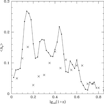
Mean value of AV as a function of redshift, for galaxies (filled circles and solid line) and quasars (crosses).
There is some tendency for aliasing between extinction and galaxy template type, and this is probably responsible for the peaks and troughs in the AV distribution.
The extinctions measured here represents an excess extinction over the standard templates used, which already have some extinction present. The average extinction in local spiral galaxies is AV∼ 0.3 (Rowan-Robinson 2003b).
We find that 9 per cent of SWIRE galaxies and 6 per cent of quasars have AV≥ 0.5. A few galaxies and quasars would have found a better fit with AV > 1, but these represent <1 per cent of the population.
The redshift solutions with extinction appear to be better than those with extinction set to zero.
8 INFRARED GALAXY POPULATIONS
Our infrared template fits, for sources with infrared excess at λ≥ 8 μm, allow us to estimate the bolometric infrared luminosity, Lir, which can be a measure of the total star formation rate in a galaxy (if there is no contribution from an AGN dust torus). Since the optical bolometric luminosity of a galaxy, corrected for extinction, is a measure of the stellar mass, the ratio Lir/Lopt is a measure of the specific star formation rate in the galaxy, ie the rate of star formation per unit mass in stars. However, there are some caveats which should be borne in mind throughout this discussion. First, uncertainties in photometric redshifts, and the possibility of catastrophic outliers, will affect the accuracy of the luminosities. Because these depend on the number of photometric bands available, they are best evaluated by reference to Fig. 11. For redshifts determined from at least five bands, the rms uncertainty in log10(1 +zphot) ≤ 0.017 and the corresponding uncertainty in luminosity at z= 0.2, 0.5, 1 and 1.5 is 0.20, 0.10, 0.07 and 0.06 dex, respectively, with a few per cent being catastrophically wrong. Secondly, if we only have data out to 24 μm we need to bear in mind that the estimate of the infrared bolometric luminosity is uncertain by a factor of ∼2 due to uncertainties in the correct template fit (Rowan-Robinson et al. 2005; Siebenmorgen & Krugel 2007; Reddy et al. 2006 quote 2-3), and this applies also to derived quantities like the star formation rate. Finally there is the issue of whether the 8–160 μm sources have been associated with the correct optical counterpart in cases of confusion. The process of band-merging of Spitzer data in the SWIRE survey and of optical association has been described by Surace et al. (2004, in preparation) and Rowan-Robinson et al. (2005). The probability of incorrect association of 3.6–24 μm sources is very low for this survey. Similarly the incidence of multiple possible associations between 3.6 and optical sources within our chosen search radius of 1.5 arcsec is very low (<1 per cent). Association of 70- and 160-μm sources with SWIRE 3.6–24 μm sources is made only if there is a 24-μm detection and with the brightest 24-μm source if there are multiple associations. A more sophisticated analysis would involve distributing the far-infrared flux between the different candidates. The impact of confusion on the subsequent discussion is expected to be small, though it may affect individual objects. It does not affect any of the more unusual classes of galaxy discussed below.
Fig. 16(L) shows the ratio Lir/Lopt versus Lir for our most-reliable subsample, galaxies with spectroscopic redshift and 70-μm detections, with different colour-coding sources dominated by cirrus, M82 or A220 starbursts or ‘AGN dust tori. Unfortunately, this sample is heavily biased to low redshifts and does not contain many examples of ultraluminous galaxies (Lir > 1012L⊙), or of galaxies with Lir/Lopt > 1.
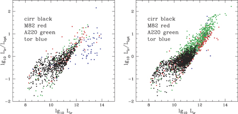
Left-hand panel: ratio of infrared to optical bolometric luminosity, log10(Lir/Lopt), versus 1–1000 μm infrared luminosity, Lir for SWIRE galaxies and quasars with spectroscopic redshifts and 70-μm detections. Right-hand panel: ratio of infrared to optical bolometric luminosity, log10(Lir/Lopt), versus 1–1000 μm infrared luminosity, Lir for SWIRE galaxies and quasars with photometric redshifts determined from at least six photometric bands and with reduced χ2 <5 and with 24- and 70-μm detections.
In Fig. 16(R), we show the same plot but we have dropped the requirement of spectroscopic redshift to that of highly reliable photometric redshifts (at least 6 photometric bands, reduced χ2 < 5). We now see large numbers of ultraluminous galaxies, especially with A220 templates. We also see a small number of cool luminous galaxies, sources with Lir > 1012 L⊙ and Lir/Lopt > 1 whose far infared spectra are fitted with a cirrus template, as was seen in the ISO ELAIS survey (Rowan-Robinson et al. 2004).
Fig. 17(L) shows Lir/Lopt versus M* for cirrus galaxies, colour-coded by optical SED type. Since the emission is due to interstellar dust heated by the general stellar radiation field, Lir/Lopt is a measure of the dust opacity of the interstellar medium. Although many galaxies with elliptical SEDs have Lir/Lopt≪ 1, consistent with low dust opacity, significant numbers of galaxies with elliptical SEDs in the optical seem to have values of Lir/Lopt comparable with spirals. There is a population of high-mass spirals with dust opacity ≥1.
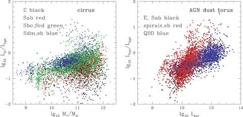
Left-hand panel: ratio of infrared to optical bolometric luminosity, log10(Lir/Lopt), versus stellar mass, M* for SWIRE galaxies with photometric redshifts determined from at least six photometric bands and with reduced χ2 < 5 and with 24-μm detections, with infrared excess fitted by cirrus template. Right-hand panel: ratio of dust torus luminosity to optical bolometric luminosity, log10(Ltor/Lopt), versus dust torus luminosity, Ltor, for SWIRE galaxies with photometric redshifts determined from at least six photometric bands and with reduced χ2 < 5 and with 24-μm detections, with infrared excess fitted by AGN dust torus template.
Fig. 18 shows the specific star formation rate, φ*/M*, versus Lir for M82 (left-hand panel) and A220 (right-hand panel) starbursts. The specific star formation rate ranges from 0.003 to 2 Gyr−1 for M82 starbursts and from 0.03 to 10 for A220 starbursts. It is by no means the case that ultraluminous starbursts are predominantly of the A220 type, as is often assumed in the literature. There is an interesting population of galaxies with elliptical SEDs in the optical, with associated starbursts in the ir luminosity range 109–1011 L⊙, similar to those found by Davoodi et al. (2006).
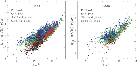
Left-hand panel: specific star formation rate, φ*/M*, in Gyr−1, versus stellar mass, M*, for SWIRE galaxies with photometric redshifts determined from at least six photometric bands and with reduced χ2 < 5 and with 24-μm detections, with infrared excess fitted by M82 template. Right-hand panel: specific star formation rate, φ*/M*, in Gyr−1, versus stellar mass, M*, for SWIRE galaxies with photometric redshifts determined from at least six photometric bands and with reduced χ2 < 5 and with 24-μm detections, with infrared excess fitted by A220 template.
Fig. 17(R) shows log10(Ltor/Lopt) versus Ltor for objects dominated by AGN dust tori at 8 μm, with different coloured symbols for different optical SED types. Ltor/Lopt can be interpreted as ftorkopt, where ftor is the covering factor of the torus and kopt is the bolometric correction that needs to be applied to the optical luminosity to acount for emission shortward of the Lyman limit. Fig. 19 shows the distribution of log10(Ltor/Lopt) for galaxies and quasars with log10Ltor > 11.5, z < 2, which is an approximately volume-limited sample. The distribution for QSOs is well fitted by a Gaussian with mean −0.10, and standard deviation 0.26.
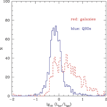
Histogram of log10(Ltor/Lopt) for QSOs (solid) and galaxies (broken).
Assuming kopt∼ 2, as implied by the composite QSO templates of Telfer et al. (2002) and Trammell et al. (2007), we deduce that the mean value of the dust covering factor ftor for quasars is 0.40. The 2σ range would be 0.1–1.0 We can use this mean value to infer the approximate luminosity of the underlying QSO in the galaxies with AGN dust tori, since LQSO∼ 2.5Ltor, and hence deduce that most of the galaxies with Ltor/Lopt > 2.5 should be type 2 objects, since the implied QSO luminosity, if it was being viewed face-on, would be sufficient to outshine the host galaxy. There are 413 such galaxies in this distribution. QSOs with Ltor/Lopt > 2 should also be type 2 objects, although they must be presumed to be cases similar to SWIRE J104409.95+585224.8 (Polletta et al. 2006), where the optical light is scattered light representing only a fraction of the total intrinsic optical output. There are 84 of these. These 497 type 2 objects can be compared with the 796 QSOs with Ltor/Lopt < 2, which are type 1 objects, yielding a type 2 fraction of 0.41, in good agreement with the covering factor deduced above.
Most of the galaxies with log10Ltor < 11.5 in Fig. 17(R) tend to lie at progressively lower values of Ltor/Lopt than the QSOs, by an amount that increases towards lower Ltor, consistent with an increasing contribution of starlight to Lopt.
Fig. 20 shows SEDs for examples of two populations of interest. Fig. 20(L) shows the SEDs of five galaxies with good quality photometric redshifts (at least six photometric bands, reduced χ2 < 5, and 24- and 70-μm detections (in two cases also 160 μm), with the infrared template fitting requiring a very luminous cool component (>1012 L⊙). The luminosity in this cool component is clearly substantially greater than the optical bolometric luminosity, suggesting that the optical depth of the interstellar medium in these galaxies is >1 (Efstathiou & Rowan-Robinson 2003; Rowan-Robinson et al. 2004).
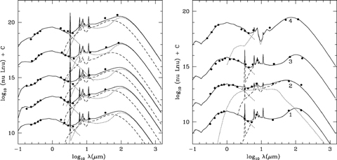
Left-hand panel: SEDs of luminous cool galaxies with good photometric redshifts (more than five photometric bands, reduced χ2 < 5) and 24- and 70-μm detections. In each case, the infrared SEDs are fitted by cirrus and M82 starburst components, with the dominant luminosity coming from the cool cirrus component. Right-hand panel: SEDs of luminous infrared galaxies with elliptical galaxy SEDs in the optical, 24-, 70- and 160-μm detections, and spectroscopic redshifts.
Fig. 20(R) shows the SEDs of four galaxies with elliptical galaxy template fits in the optical, spectroscopic redshifts and Lir > Lopt. These are galaxies that in optical surveys would be classified as red, early-type galaxies. In the infrared two are fitted by cirrus components (objects 1 and 3), one by an Arp220 starburst (object 4) and one by a combination of an AGN dust torus and an M82 starburst (object 2). Since highly extinguished starbursts like Arp220, which are probably the product of a major merger, do look like ellipticals in the optical because the optical light from the young stars is almost completely extinguished, object 4 is consistent with being a highly obscured starburst. For object 2, an elliptical galaxy SED in the optical coupled with an AGN dust torus in the mid infrared implies the presence of a type 2 QSO, in which the QSO is hidden behind the dust torus. The infrared SED of this object (object 2) also shows evidence for strong star formation, so this also appears to be a case of an obscured starburst. The two galaxies with elliptical-like SEDs in the optical and with strong cirrus components (objects 1 and 3) are harder to understand. If the emission is from interstellar dust and the dust were being illuminated solely by the old stellar population, then a high optical depth would be implied by the fact that Lir > Lopt, but the optical SED shows no evidence of extinction. The implication is that they are probably also obscured starbursts, perhaps with star formation extended through the galaxy to account for the form of the infrared SED. To see whether the morphology can help the interpretation, we show in Fig. 21 IRAC images of these four galaxies, colour-coded as blue for 3.6 μm and red for 8 μm. Objects 1 and 2 look elliptical and object 3 looks lenticular. All three are strongly reddened in their outer parts, indicating that the long wavelength radiation is coming from the outer parts of the galaxies. This suggests that the infrared emission is associated with infalling gas and dust. Object 4 appears more compact, consistent with being similar to Arp 220.
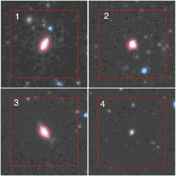
Postage stamps for the four elliptical galaxies of Fig. 19(R), colour-coded with blue = 3.6 μm, red = 8 μm. The size of each postage stamp is 1 arcmin.
Fig. 22R shows the specific star formation rate versus stellar mass for 4135 SWIRE galaxies with 1.5 < zphot < 2.5, 24 μm detections and ir excesses in at least two bands, and reduced χ2ν < 5. This can be contrasted with fig. 15 of Reddy et al. (2006), based on 200 galaxies identified by Lyman drop-out and near-infrared excess techniques. SWIRE is clearly a source of high-redshift galaxies with infrared data which far exceeds previous optical-based samples. Compared with the Reddy et al. (2007) we note that in the range log10M*/M⊙∼ 11–12), we find a far larger range of specific star formation rate. Because the depth of our optical surveys is typically r∼ 23.5–25, we do not sample the low-mass end of the galaxy distribution at these redshifts as well as Reddy et al. (2006).
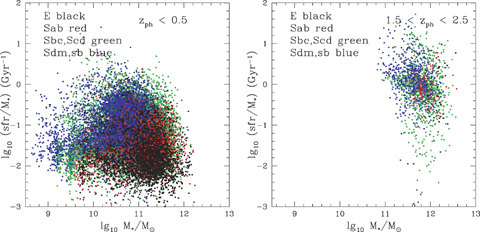
The specific star formation rate φ*/M*, versus stellar mass, M*, for galaxies with (L) z < 0.5, (R)1.5 < zphot < 2.5, colour-coded by optical SED type.
Fig. 22(L) shows the same plot for z < 0.5. We see that at the present epoch specific star formation rates >1 Gyr−1 are rare, whereas they seem to have been common, at least amongst massive galaxies, at z∼ 2. At low redshifts, we see some evidence for ‘downsizing’, in that elliptical galaxies, which tend to be of higher mass, have significantly lower specific star formation rates than lower mass galaxies, which tend to have late-type spiral or starburst SEDs.
Fig. 23L shows the star formation rate φ* against redshift. Although the distribution is subject to strong selection effects, with the minimum detectable φ* increasing steeply with redshift to z∼ 2 and then decreasing towards higher redshift because of the negative K-correction at 8 μm, the plot is consistent with a star formation history in which the star formation rate increases form z= 0–1.5 and then remains steady from z= 1.5–3.
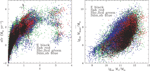
Left-hand panel: the star formation rate φ*, in M⊙ yr−1, versus redshift, colour-coded by optical SED type. Right-hand panel: the dust mass, Mdust/M⊙ versus stellar mass, M*, for SWIRE galaxies, colour-coded by optical SED type.

These dust masses have been given in the catalogue (section 5) and Fig. 23(R) shows the dust mass, Mdust, versus the stellar mass, M*, for SWIRE galaxies, coded by optical SED type. For most galaxies Mdust/M* ranges from 10−6 to 10−2, with the expected progression through this ratio with Hubble type. Galaxies with exceptionally high values of this ratio presumably have gas masses comparable to the stellar mass, assuming the usual gas-to-dust ratios. The dust masses will be uncertain because the uncertainty in photometric redshifts makes luminosities uncertain by a factor ranging from 0.06 dex at z= 1 to 0.20 dex at z= 0.2 (see start of this section). There will also be a larger uncertainty associated with ambiguity in the template fitting. To estimate this, we looked at all fits to the infrared excess where there is an excess in at least two bands, excluding cases with an AGN dust torus component, and with reduced χ2 for the infrared fit <5. Relative to the best-fitting dust mass, we find an rms uncertainty of ±0.8 dex, or a factor of 6, so these dust mass estimates have to be treated with caution. This uncertainty is substantially reduced if 70- or 160-μm data are available. Data from Herschel will allow these dust mass estimates to be greatly improved.
9 CONCLUSIONS
We have presented the SWIRE Photometric Redshift Catalogue 1 025 119 redshifts of unprecedented reliability and good accuracy. Our methodology is an extension of earlier work by Rowan-Robinson (2003a), Rowan-Robinson et al. (2004, 2005) and Babbedge et al. (2004) and is based on fixed galaxy and QSO templates applied to data at 0.36–4.5 μm, and on a set of four infrared emission templates fitted to infrared excess data at 3.6–170 μm. The galaxy templates are initially empirical, but have been given greater physical validity by fitting star formation histories to them. The code involves two passes through the data, to try to optimize recognition of AGN dust tori. A few carefully justified priors are used and are the key to suppression of outliers. Extinction, AV, is allowed as a free parameter. We have provided the full reduced χ2ν (z) distribution for each source, so that the full error distribution can be used, and aliases investigated
We use a set of 5982 spectroscopic redshifts taken from the VVDS survey (Le Févre et al. 2004), the ELAIS survey (Rowan-Robinson 2003a), the SLOAN survey, NED, our own spectroscopic surveys (Smith et al., in preparation; Trichas et al., in preparation; Swinbank et al. 2007) to analyse the performance of our method as a function of the number of photometric bands used in the solution and the reduced χ2ν. For seven photometric bands (5 optical + 3.6, 4.5 μm), the rms value of (zphot−zspec)/(1 +zspec) is 3.5 per cent, and the percentage of catastrophic outliers (defined as >15 per cent error in 1 +z) is ∼1 per cent. These rms values are comparable with those achieved by the COMBO-17 collaboration (Wolf et al. 2004), and the outlier fraction is significantly better. The inclusion of the 3.6- and 4.5-μm IRAC bands is crucial in suppression of outliers.
We have shown the redshift distributions at 3.6 and 24 μm. In individual fields, structure in the redshift distribution corresponds to real large-scale structure which can be seen in the spectroscopic redshift distribution, so these redshifts are a powerful tool for large-scale structure studies.
10 per cent of sources in the SWIRE photometric redshift catalogue have z > 2, and 4 per cent have z > 3, so this catalogue is a huge resource for high-redshift galaxies. The redshift calibration is less reliable at z > 2 and high-redshift sources often have significant aliases, because the sources are detected in fewer bands.
We have shown the distribution of the mean extinction, AV, as a function of redshift. It shows a peak at z∼ 0.5–1.5 and then a decline to higher redshift, as expected from the star formation history for galaxies.
A key parameter for understanding the evolutionary status of infrared galaxies is Lir/Lopt, which can be analysed by optical and infrared template type. For cirrus galaxies this ratio is a measure of the mean extinction in the interstellar medium of the galaxy. There appears to be a population of ultraluminous galaxies with cool dust and we have shown SEDs for some of the reliable examples. For starbursts Lir/Lopt can be converted to the specific star formation rate. Although the very highest values of this ratio tend to be associated with Arp220 starbursts, by no means all ultraluminous galaxies are. There is a population of galaxies with elliptical SEDs in the optical and with luminous starbursts, and we have shown SEDs for four of these with data in all Spitzer bands and spectroscopic redshifts. For three of them, the IRAC colour-coded images show that the 8-μm emission is coming from the outer regions of the galaxies, suggesting that the star formation is associated with infalling gas and dust.
Analysis of the VVDS area was based on observations obtained with MegaPrime/MegaCam, a joint project of CFHT and CEA/DAPNIA, at the Canada–France–Hawaii Telescope (CFHT) which is operated by the National Research Council (NRC) of Canada, the Institut National des Sciences de L'Univers of the Centre National de la Recherche Scientifique (CNRS) of France, and the University of Hawaii. The work is based in part on data products produced at TERAPIX and the Canadian Astronomy Data Centre as part of the Canada–France–Hawaii Telescope Legacy Survey, a collaborative project of NRC and CNRS.
We are grateful for financial support from NASA and from PPARC/STFC.
We thank Max Pettini for helpful comments.
REFERENCES
