Analytic central orbits and their transformation group Free

Abstract

1 INTRODUCTION

Since schooldays when we encountered the rigid pendulum, most of us have been frustrated by our inability to integrate in elementary terms Abelian expressions of the form ⁠, where S(u) has simple zeros at u_a and u_p≥u_a but is not quadratic. In practice S usually depends linearly or quadratically on parameters which we shall call ɛ and h, and its zeros u_p and u_a depend on ɛ and h often in quite complicated ways. In Appendix A we relieve this frustration by showing how for each pair of u_a and u_p, S may be replaced at lowest order by a quadratic function with the same zeros and the integral may be approximately evaluated parametrically via perturbation theory.

We do not have to solve S(ɛ, h, u) for its zeros u_p and u_a. Instead we regard u_p and u_a as parameters and then easily find the ɛ(u_a, u_p) and h(u_a, u_p) to which they correspond. The process of replacing S by a different quadratic function for each pair of zeros u_p and u_a we call quadrating (after the old verb ‘to quadrate’ which means ‘to make square’). Surely using ‘quadrate’ to mean ‘to make quadratic’ is not too great an extension! As the simple, though crude, method developed can be applied to a far wider class of problems than those encountered here, we have mentioned it first in Section 1.

Orbits of the general form

1

have a long history. Newton in Principia (1687) showed that orbits of this form with k= 1 occurred when the central force was an inverse-square law supplemented by an inverse cube force. His celebrated theorem on revolving orbits demonstrates that if r=r(φ) is an orbit of angular momentum h under any central force ⁠, then r=r(mφ) is an orbit of angular momentum m h under the central force ⁠. Newton also pointed out that r(t) was the same for both orbits, so, if the new orbit were viewed from axes revolving at the rate ⁠, then the two orbits would have the same shape. But note that is not a constant rotation rate, but speeds up when r is small and slows down when r is large. When we view the orbit from axes that rotate uniformly at the same mean rate ⁠, the orbits can have very different shapes involving figures of eight for the more eccentric ones (Lynden-Bell & Lynden-Bell 1995).

Recently in a fine paper, Struck (2006) showed that orbits of moderate or low eccentricity in logarithmic or power-law potentials with or without cores were well approximated by analytic orbits of the form (1). His approximate orbits are surprisingly accurate. Struck was, in part, stimulated to find this result by a paper by Touma & Tremaine (1997) that demonstrated the richness of the resonances in the perturbation theory of these systems. Valluri et al. (2005) have emphasized that the apsidal precession found in non-inverse-square orbits is significantly dependent on the eccentricity of the orbit involved.

Surprisingly, we have been led to orbits of the form (1) by looking at orbits of extreme eccentricity e= 1, where Struck's methods did not give accurate results. Standard works on orbits, Boccaletti & Pucacco (1996), Contopoulos (2002) and Binney & Tremaine (1987), do not point out that the orbits of zero energy in power-law potentials can be exactly solved analytically. The same variables can be used to solve the nearly circular orbits. Since both highly eccentric and small eccentricity orbits can be so solved, it would be surprising if there were not a good approximation, based on the same variables, that interpolated between e= 1 and 0. Struck's methods do this well for small and moderate eccentricities. Here we show that all orbits are well approximated by analytic orbits of the form (1) for 0 ≤e≤ 1.

Here ℓ and e are generalizations of the semi-latus-rectum and the eccentricity. The potential is Ar^−α=Ar^k−2; this parametrization, using k rather than α, is chosen in this section to simplify equations (2) and (3) below. If r_a and r_p are the apocentric and pericentric distances, the generalized eccentricity is given by

2

and the generalized semi-latus-rectum is given by ℓ where

3

We note that for the Kepler case k= 1 and the above formulae all reduce to the usual ones. We write ℓ=Lr_c, where r_c(h) is the radius of the circular orbit of angular momentum h. We have r^k_c= (2 −k)⁻¹h²/A. The dimensionless parameters L and m are functions of e. Orbits of small eccentricity have ⁠, while those with e= 1 have m=k. We find the orbits in the −V² ln r potential from the limiting case k→ 2.

In Appendix A we show how to improve the accuracy of our orbits via perturbation theory; however, for most purposes the simplicity of the initial approximation (1) outweighs the extra complication that accompanies greater accuracy. Our methods can be applied to non-power-law potentials (see Kalnajs 1979) but here, for simplicity, we limit ourselves to power laws.

While our methods can be extended to unbound orbits, the results are less pleasing so they are consigned to Appendix B.

In Section 3 we use the transformation theory of Newton, Bohlin, Arnold and others to transform our orbits for 0 < k < 2 into orbits in potentials with positive powers of r. We show how that theory can be extended naturally to give a set of transformations that form a group. We develop the subgroup of switch transformations and show that orbits in the potentials ψ∝r^k−2 are conjugate to orbits in the potentials r^2(2−k)/k, r^−k, r^2k/(2−k), r^−4/k and r^−4/(2−k). These transformations are not restricted to power laws, although special simplifications occur for them. Applications are made to Plummer's law.

It is shown that the full group has a transformation that connects the Keplerian potential to the isochrone.

2 ANALYTIC ORBITS

2.1 General orbits in potentials with 0 < k < 2

Those looking for orbits in potentials with powers k outside the above range should consult Section 3.

A general orbit of specific energy ɛ and specific angular momentum h in the power-law potential ψ=Ar^k−2 has, in the usual notation, and

Now

4

In place of r we shall use a dimensionless variable which generalizes the u(=1/r), so useful in the Keplerian case:

5

We also define a dimensionless energy

6

Now k dr/r=−du/u so we may rewrite (4) in terms of u:

7

where

8

and σ= 2(k− 1)/k, which is less than one for 0 < k < 2. For the marginally bound orbits ɛ= 0, the u^σ term in (8) disappears so we may integrate (7) exactly. Substituting u= 1 + cos η reduces (7) to k dφ= dη. Choosing the zero of φ at that pericentre where η= 0, we have η=kφ, so the solution for the orbit is of the form of equation (1) with e= 1 and m=k:

Indeed, it was this result that motivated our choice of u as the basic variable. Nearly circular orbits can also be nicely treated in terms of u, so this encouraged us to conjecture that all bound orbits can be found analytically to good accuracy.

Our analytic strategy for integrating equation (7) more generally is to replace S(u) with a quadratic function S_Q(u), which has precisely the same zeros, u_a and u_p, corresponding to the apocentre and pericentre of the orbit. Thus S_Q=q²(u_p−u)(u−u_a) whose q², the coefficient of −u² in S_Q, is to be determined so that in some average sense S_Q(u) is a good approximation to S(u) in the radial range u_p≥u≥u_a occupied by the orbit. For example, we find that choosing q² so that gives a q that is good to 2 per cent accuracy. A better choice, given later, is the natural starting point for the perturbation theory of Appendix A.

Once S(u) in equation (7) has been replaced by the quadratic S_Q(u), the integration is easy. From (2), e= (u_p−u_a)/(u_p+u_a), so one sets and it follows that so ⁠. If we make the substitution ⁠, we find that the integration of (7) gives qkφ=η, so the orbit is

which is of the form (1) with m=qk.

Crucial to this method of solving for the orbits is the knowledge of u_p and u_a. A critical step in finding them is to regard the r_p and r_a of an orbit as given, in place of its energy and angular momentum. Those can easily be found if r_p and r_a are given, but solving the other way around is usually difficult. Once the orbit has been found, this approximation allows us to determine the radial action and hence the time from pericentre to a given point on the orbit.

Having outlined our general procedure, we now turn to solving the circular and nearly circular orbits using u, rather than r, as the variable.

2.2 Nearly circular orbits

For the circular orbits of angular momentum h, the centrifugal force balances gravity, so h²r⁻³_c=−dψ/dr= (2 −k) Ar^k−3_c and so for them u=u_c= 2 −k. Also since is zero for them their energy is ɛ_c where

Also S(u_c) = 0, so in our dimensionless variables, cf. equation (8),

9

We consider first orbits with energies not much above E_c and we set

10

then Δ is small for nearly circular orbits and one at the energy of escape.

where E_c is given by (9). For the nearly circular orbits, we expand the obstreperous u^σ term in (8) about u=u_c, omitting terms higher than quadratic in u−u_c:

so inserting this result into (8),

where again the coefficient of −u² in S_Q is q² and here

11

Completing the square on ⁠, we have

12

where and

13

Integrating (7) with S given by (12) by writing yields

14

so the orbits take the form (1) with m=kq. Note that as Δ→ 0, q→k^−1/2 and ⁠.

Whereas these formulae have been derived by neglecting the (u−u_c)³ and higher terms in the expansion of u^σ, it should be realized that the coefficient of the u^σ term itself vanishes at the energy of escape. Thus, despite this neglect, our formulae are exact, not just for Δ small, but also at Δ= 1. Indeed at Δ= 1 we see that and e= 1. However, even such partial reassurance should not deceive us into believing that formulae (11) and (13) are good enough at intermediate values of e.

2.3 Analysis of general orbits

In the non-linear regime, we see from the e= 1 orbits that u has its mean at 1 rather than at 2 −k. It makes little sense to expand u^σ about u_c= 2 −k when Δ is not small. Nevertheless we would like to quadrate S, that is, approximate S(u) by some quadratic function. We adopt a very different procedure in the non-linear case. In place of fixing the energy and the angular momentum of an orbit and then determining its shape and size, we choose, instead, a pericentric distance r_p and an apocentric distance r_a. From these it is simple to find exactly what energy and angular momentum are needed. Equivalently we can fix the values of ℓ and e so then r_p=ℓ/(1 +e)^1/k and r_a=ℓ/(1 −e)^1/k, as can be seen from (1) with mφ equal to first 0 and then π.

Since at both r_p and r_a, we have for ɛ < 0

15

16

which we may solve for h² and ɛ in terms of r_a and r_p or, alternatively, in terms of ℓ and e:

17

Multiplying (15) by r²_p and subtracting from it r²_a×(16), we deduce

18

Another alternative, which is the most useful one in the equivalent problem in quantum mechanics, is to consider h and e as given. Then, eliminating ℓ in (18) in favour of h as found from (17), we obtain

where, setting γ= (2 −k)/k,

19

Despite its strange appearance, g(e) is not a complicated function. For k= 1 it is ½(1 −e²) and for k= 2 it is 1. We plot g against 1 −e² for several k values in Fig. 1.

Figure 1

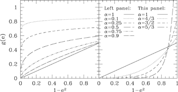
The function g(e) for various values of α= 2 −k. g(e) is minus the dimensionless energy E. As α→ 0, the graph tends to the line g(e) ≡ 1.

Open in new tabDownload slide

We wish to approximate S by a quadratic in u which must vanish at u=u_p and u_a, so it has to take the form

20

where q is yet to be determined and has been given that notation to conform with our earlier definition that −q² is the coefficient of u² in S. In the above,

21

from which we see that is twice the final expression in (17) but without the ℓ^k. The ‘eccentricity’e is (u_p−u_a)/(u_p+u_a) as always. Using (20) for S(u) with the substitution ⁠, we readily integrate equation (7) to obtain qkφ=η as before. So the solution is still equation (1) with m=qk, but we must still determine q².

A useful approximate formula, good to about 2 per cent, is given by setting ⁠. This gives, for σ≠ 1/2 (i.e. α≠ 2/3),

22

with m=qk as before and can be expressed as a function of k and e only, via (17) and (21). We have chosen this power of u in the integrals we equate above, as it gives the best agreement to the true m without compromising on the simplicity of the expression for q. We note that choosing u⁻¹ in the integrals gives as good an agreement as using u^−3/2, but with the resulting m becoming overestimates on the true value for α < 1 and vice versa for α > 1. Choosing an exponent between −1 and −1.5 results in better agreement still, but we lose the simplicity of the resulting analytic expression for q. The exponent of −4/3 is as good as any, but gives the following somewhat awkward result:

where e_±= (1 ±e)^1/3.

The angle between successive apocentres is important as such angles accumulate as the orbit is prolonged. We now determine q to get this angle as accurately as possible. It is given by

hence the average of (S_Q/S)^1/2 over η must be 1. We evaluate this average over eight points around −π < η < π. There is a difficulty in evaluating (S_Q/S)^1/2 exactly at the apocentre when e= 1 since the apocentre is at infinity. Surprisingly, the result of taking the limit of r_a as e→ 1 gives a different (and wrong) result from setting e= 1 and then evaluating the limit as cos η→−1. We get around this by using cos η=−0.990, where everything is finite, in place of η=π.

At pericentre u_p, both S_Q and S are zero but the limit of is

We evaluate

where ⁠, at the other seven points ±π/4, ±π/2, ±3π/4 and cos η=−0.990. For convenience, we label the values of u at ±π/4 and ± 3π/4 as and ⁠, respectively. Our estimate of 1/q is the average over the eight values that result:

23

At each α, the resulting q is a (somewhat complicated) function of e, since are all functions of e.

2.4 Comparisons with computed orbits

Orbits were computed in the xy plane from the Cartesian form of the equations of motion for potentials with α= 0.25, 0.55, 0.75, 1.5 and 1.0. The last provides a valuable check that we get m= 1 in the Newtonian case, even at very high eccentricities of order 0.999. We also checked that for nearly circular orbits and that m→k as e→ 1 for all the values of α. As m varies quite rapidly with eccentricity as e→ 1, accurate computations are required at high eccentricities. Orbits in the logarithmic potential which gives a constant circular velocity are considered later, in Section 2.6; the approximation adopted there is somewhat different.

Fig. 2 shows a comparison between our estimated values of m and the computed values of m for potentials with α= 0.25, 0.55, 0.75 and 1.5. For all values of α shown, the deviation of m calculated from the analytical formula (23) is only a fraction of a per cent. Note that both plots are against so that high eccentricities are on the left-hand side and low eccentricities are on the right-hand side. It is, of course, possible to read off m as a function of or of e from the computed points in this figure.

Figure 2

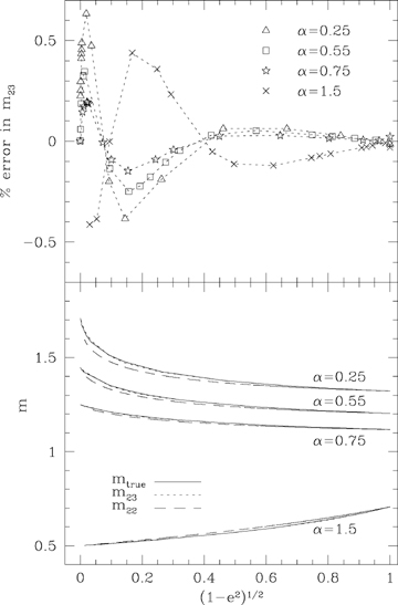
The top panel shows the percentage difference between the true value of m from computed orbits and m₂₃ calculated from the analytical formula (23), plotted as functions of for different values of 2 −k=α. The largest deviations occur at high eccentricities; the region 0.1–0.3 in corresponds to 0.995 > e > 0.954. The bottom panel shows the values of m, estimated using (22) and (23), along with the true values, again for four values of α.

Open in new tabDownload slide

Panel (a) of Fig. 3 shows a computed orbit in the potential with α= 0.25 together with an orbit of the same m, r_a and r_p but calculated from the equation (ℓ/r)^k= 1 +e cos (mφ). This demonstrates how the shape given by equation (1) fits the computed orbit. A better fit is obtained using the perturbation theory of Appendix A. The dotted orbit in panel (b) is (ℓ/r)^k= 1 +e cos(m₂₃φ) and the gradual precession due to the error in the estimated m₂₃ is readily seen.

Figure 3

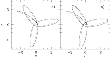
An orbit in the 2 −k=α= 0.25 potential, chosen to be in the high-eccentricity region where the approximation is least good. The full line is the computed true orbit. In panel (a), it is compared to (ℓ/r)^k= 1 +e cos(mφ) (dotted line) with m chosen to agree with the computed orbit. This shows the deviation in the shape of the lobes. In panel (b), the value of m is estimated by the 8-point average of equation (23) and the error in m is readily seen from the different precession of the solid and dotted orbits. The difference in the true value of m and that estimated from the 8-point average is less than 0.5 per cent. All orbits start at the starred location.

Open in new tabDownload slide

Fig. 4 shows two orbits with the same ratio of r_a/r_p but in the potentials with α= 0.55 and α= 0.75. Because the definition of ‘eccentricity’ we gave in equation (2) depends on α (through k), these orbits have eccentricities of 0.662 and 0.596, respectively. Note that the two drawings have the same number of apsides but these have precessed much less for the α= 0.75 orbit as the potential is closer to the Keplerian α= 1.

Figure 4

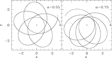
Two computed orbits with the same r_min/r_max in potentials with different 2 −k=α are compared with the analytic orbits (ℓ/r)^k= 1 +e cos (m_trueφ) (dotted lines). The α= 0.55 orbit has e= 0.662 while the α= 0.75 orbit has e= 0.596 and precesses much less rapidly. Both the shapes and the precession rates of these orbits are well represented by the analytic formula.

Open in new tabDownload slide

Fig. 5 shows two orbits in the α= 1.5 potential for which the precession is forwards because α > 1 whereas the other illustrations all have a backward precession. Under the transformation ζ=z^k/2 considered in Section 3, these orbits transform into ones in the potentials ψ∝r^2α/k=r⁶. For orbits with α > 1, the straight perturbation theory giving m=kq with q given by (23) yields m to better than 0.5 per cent.

Figure 5

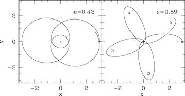
Two orbits in the 2 −k=α= 1.5 potential. The orbit on the left-hand side has a forward precession by nearly 180° whilst that on the right-hand side has a forward precession by a little over 270°. The turn close to the origin in the latter cannot be seen but is a more rapidly turning version of that seen on the left-hand side. The lobes are numbered in sequential order for the higher eccentricity orbit.

Open in new tabDownload slide

It is often useful to have a vectorial way of delineating orbits and the velocities of particles describing them. To do this, we generalize Hamilton's eccentricity vector which has magnitude e and points towards pericentre. As our pericentres precess within the orbital plane, we invent a rotating eccentricity vector. If we start at pericentre with e=e₀ we take e at later times to be given by ⁠. This e obeys ⁠. The angle between the radius vector to the particle and the eccentricity vector is then mφ and the equation of the orbit (1) can be rewritten as

24

The transverse velocity of the particle is clearly and the radial velocity can be obtained from the orbit and the energy equation. Using our approximations quadrating the latter, we find

25

Given v and r at one time one might wish to use these equations at a later time. Then one needs to find e, h, ℓ, q and m from the initial v and r together with the known potential ψ=Ar^−α. From v and r it is easy to construct ɛ=½v²−Ar^−α and h=r×v, from these E is found. For given E and α, e may be found from Fig. 1. ℓ then follows from (17) and m, q from (23). The direction of e within the plane perpendicular to h then follows from with the ambiguity in angle resolved from which follows from the v equation above. Thus all the orbital parameters are determined.

2.5 Action, adiabatic invariants and time

So far we have concentrated on the shape of the orbit in space; however, the time from pericentre to any point of the orbit is just as important. Both can be obtained from the action function S_r, whose relationship to S(u) is given below.

26

If we now use our quadratic approximation we find

setting ⁠, this becomes, setting f= 1/e,

Now the related integral

and the integral that we want is just − d/d f of this, so

27

so, putting this in S_r and remembering that f= 1/e,

28

The adiabatic invariant is given by

29

Now

where P_r is the radial period while

J_r/h is a function of eccentricity, so the partial differentiation is best done via

and

30

so this expression gives the time to any chosen point in the orbit. In practice, S_r/h is a function of e and η, so the partial derivative is calculated using

In the general case, use of 1/u∝r^k as a variable does not lead to a prettier equation for t, such as the one Kepler derived for k= 1, but see the next section for logarithmic potentials.

In the equatorial plane the total action is S_A=S_r+h_zφ. The action variables are J_r and h_z=h. The angle variables are the phases of the oscillations in r and φ and are given by w_r=∂S_A/∂J_r and w_φ=∂S_A/∂h. For general orbits, the action variables are most often employed when the potential is of the more general separable form ψ=Ar^−α−B(θ)/r²; h² is no longer conserved but I=h²− 2B(θ) is. The general action is then S_A=S_r+S_θ+h_zφ with and J_θ= 1/(2π)∮∂S_θ/∂θdθ. The angle variables are w_θ=∂S_A/∂J_θ and w_φ=∂S_A/∂h_z.

2.6 Logarithmic potentials α→ 0

For small α we write and expand to obtain ψ=Ar^α₀ [1 −α ln (r/r₀) + 0 (α²)]. We set A=V²/α and consider taking the limit as α→ 0 while keeping V² fixed so A tends to infinity. To keep a finite potential, we have to subtract the constant Ar^−α₀ from ψ, so we obtain a new potential

To apply the methods of Section 2.1, we define

and consider orbits defined by pericentric and apocentric distances r_p and r_a. In place of equations (15) and (16) we then have

31

32

and

33

The orbital equation reads

where

34

and E=ɛ/V² which is given in terms of e via (33). We now approximate S_L(u) by the quadratic (20), which shares the same zeros.

As in Section 2.3, a useful analytic expression for q is given by again equating

to

where is given by (32). This yields

35

This expression is good to 2 per cent. Once again, more accurately we calculate q⁻¹ from the average of over η, where ⁠. At u_p,

36

37

where ⁠. As found in Section 2.3, the apocentre once again poses a problem and we evaluate

38

at where λ=−0.990, as before, and where S_L(u) is given by (34). So a 4-point estimate of q is given by

39

and an 8-point estimate is likewise

40

where S_±=S_L and ⁠. Fig. 6 shows the contribution of each point in (39) and (40) along with a comparison of the true m and the value derived from the 8-point estimate via m₄₀=q₈k. Fig. 7 compares an approximate orbit to a computed one.

Figure 6

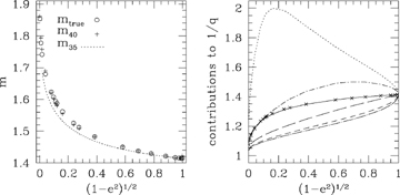
The left-hand panel shows a comparison between the true value of m (open circles) and that estimated from equation (35), which gives m to better than 2 per cent, and the 8-point average in equation (40), which gives m to better than 1 per cent. The right-hand panel shows (in thick solid) the true value of 1/q=k/m overlaid (in crosses) with that derived from the 8-point average. The agreement is clearly good to a fraction of a per cent. The individual contributions made by each of the points given in the terms of equations (39) and (40) are also shown. From the top, the various lines correspond to u_a (dotted), u₊ (dot–short-dashed), (long-dashed), u₋ (short-dashed) and u_p (dot–long-dashed).

Open in new tabDownload slide

Figure 7

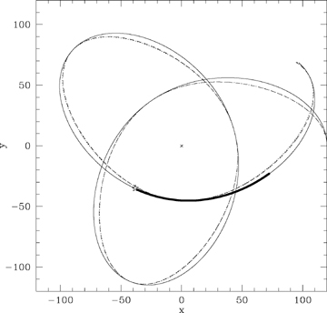
An orbit in the logarithmic potential. The solid line is the computed orbit, and the dotted line shows the approximate orbit (ℓ/r)²= 1 +e cos(m_trueφ). Overlaid (and hardly visible) is a dashed line showing an orbit with the estimated m, calculated from (40), instead of m_true. The error in this value of m is less than 0.1 per cent. The heavy line shows the piece of such an orbit for the trailing Magellanic Stream, with the location of the Magellanic Clouds indicated by the open star.

Open in new tabDownload slide

The time to a given point in the orbit is given by

41

so the radial period is given by

42

However, a much more interesting result comes from following Kepler, whose equation comes, not from integrating the u equation directly, but by first making the substitution v= 1/u=V²h⁻²r². This gives

where we have written and ⁠; setting we see that

43

so with this approximation r² vibrates harmonically. Fig. 8 shows the computed r²(t) for an orbit together with the harmonic approximation. The adiabatic invariant is given by ⁠. This integral was evaluated in equation (28), so for this case k= 2 and

44

Figure 8

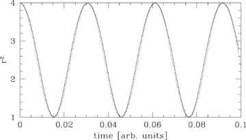
The almost simple harmonic variation of r² as a function of time in an orbit with r_a/r_p= 2 in the logarithmic potential. The dotted line is a sinusoid of the same period.

Open in new tabDownload slide

It should be emphasized that while we have set ourselves the target of getting analytical formulae that give m to 1 per cent or better for all eccentricities, we have not paid attention to minimizing errors in the temporal periods. We find that such errors are indeed higher and no doubt our formulae could be improved upon by a study of such errors.

3 TRANSFORMATION THEORY

Newton (1687) realized that the ellipse was a possible orbit both in a harmonic central potential and in an inverse-square law. In the first case the centre of force is at the centre of the ellipse, while in the latter case it is at the focus. This led him to pose the question under what circumstances can the same curve be the trajectory of a particle under a force from one of two different centres. Newton's (1714) discussion of this is well described in Chandrasekhar's (1995) book, as well as in later work by Bohlin (1911), Levi-Cìvita (1924) and Arnold (1990). All demonstrate the transformation that converts the harmonic ellipse into the Kepler ellipse and vice versa. Collas (1981) gave the relationship between equivalent potentials. Here we show that this transformation, S₁, can be embedded into a larger set of transformations that form a group. We mainly concentrate on the subgroup of switch transformations which have six members but which give just three related potentials r⁻¹, r² and r⁻⁴ in the Kepler case, since r⁻¹ is self-conjugate under one of the transformations. In the complete group, these potentials are also related to the isochrone (Henon 1959).

The energy equation of a central orbit of angular momentum h in a potential ψ(r) can be written

45

Now consider the transformation ⁠. Setting F=ρ′τ we find

46

For this to be an orbital equation like (45), the three terms on the right-hand side must be and ⁠, but not necessarily in that order.

The transformation S₁ that leads to the Newton–Levi-Cìvita–Arnold result is found by taking ⁠, identifying the last terms but switching the roles of the other two. Thus for S₁ we set

47

so we obtain the transformation

48

with ⁠. Applying this to the power-law potential ψ=Ar^−α yields so (note: α= 1 gives ⁠) the quantity in square brackets is, of course, constant. However, we could alternatively leave the first term on the right-hand side of (46), identifying it with but switching the roles of the other two terms. This leads us to the transformation S₂ in which

from which we deduce and ⁠, where

So S₂ is an inversion accompanied by the change in potential (for power laws). More generally we may ask that but that the three terms and that constitute this quantity are independent linear combinations of F²ψ, F²ɛ and ⁠. If one applies two of this more general class of transformations one after the other, it is simple to see that the net result is a transformation of this class, that the identity transformation belongs to the class and that every transformation has a unique inverse in the class. These transformations form a group in the sense of group theory, since they clearly obey the associative law

Each transformation now gives a new in the new potential that corresponds to the old r(t) in the old potential ψ. To get the transformation of φ we remember that and for so under the transformation S₁ using (46) and (47)

but from (48) so

This equation takes a particularly simple form when is a power of r, for then ⁠. Furthermore, this occurs if and only if ψ follows a power law in r; so

Note that the new potential depends on the energy of the old orbit, so a pair of orbits of different energies in the old potential will map into a pair of orbits in two different new potentials that differ by a constant factor, cf. Rosquist & Pucacco (1995). If we write z=re^iφ and then, from the above, the S₁ mapping is of the form ⁠, i.e. a conformal map in the complex plane. In general, a closed orbit will map into an unclosed Lissajoux rosette, but when 1 −α/2 =N₁/N₂ where N₁ and N₂ are relatively prime integers, then the transformation of an orbit that closes after one turn will be an orbit that closes after N₂ turns which has N₁ times as many apsides.

For α= 1, we have the famous example that transforms Kepler's ellipse into the simple harmonic oscillator. This is

If we apply S₁ again, this time starting with we find

so apart from a possible rescaling, the double transformation S²₁ leads us back to the beginning. This is true generally, not just for power laws, since from equation (48),

We shall ignore the dull rescalings in what follows and write S²₁=I, the identity. This is in agreement with the concept that a repeated switch leads to no transformation.

We now apply the transformation S₁ to orbits in one of our potentials ψ=A r^−α with 0 < α < 2. The new potential will be ⁠, which will be a positive power of and the transformed orbit takes the form

which is indeed an ellipse when m=k as for the Kepler case, which transforms to the harmonic potential. Remarkably, it is always on the left-hand side whatever α we start from, but the values of 2m/k vary with α.

S₁ is the basis for the regularization of the close encounters of two bodies carried out in three dimensions by Kustaanheimo & Stiefel (1965).

3.1 The switch subgroup

If we try to find a transformation that switches the angular momentum and potential terms in (46) while leaving the energy term unchanged, we fail because and with F constant we are unable to accomplish the desired switch.

However, we may apply first S₁ and then S₂:

This transformation is not the one we obtain by applying S₂ first and then S₁:

Applying this double transformation twice gives

which is the same as S₂S₁ up to constants of proportionality, while a further application of S₁S₂ gives

so the triple application of S₁S₂ gives a multiple of the identity.

Before going any further, let us see where we can get if we start with ψ∝ 1/r. We can get to ψ∝r² and back using S₁, but using S₂ leaves ⁠, so Newton's law is invariant under S₂. However, S₂ acting on r² leads to ⁠, but a further application of S₁ leaves r⁻⁴ invariant. Thus under the transformations considered so far, there are conjugate orbits in the r⁻¹, r² and r⁻⁴ potentials. More generally, if we start with ψ∝r^−α, then S₁ gets us to ψ∝r^2α/(2−α) (where we have dropped the tildes), while S₂ brings us to ψ∝r^α−2. The double transformations S₂S₁ and S₁S₂ give ψ∝r^{−4/(2−α)} and r^2(2−α)/α, respectively, while S₁S₂S₁ leads to ψ∝r^−4/α. Further applications only bring us back to potentials already included. In fact, there are six transformations in this subgroup, yielding a conjugacy of orbits in the six potentials r^−α, r^2α/(2−α), r^α−2, r^{−4/(2−α)}, r^2(2−α)/α and r^−4/α. For α=−1, these are r, r^−2/3, r⁻³, r^−4/3, r⁻⁶ and r⁴. For α= 1/2, they are r^−1/2, r^2/3, r^−3/2, r^−8/3, r⁶ and r⁻⁸. These powers become somewhat bizarre for small α.

degeneracies similar to those for the Kepler potential occur for α= 1, 4 or ±2.

The simple relationship holds only for power-law potentials under the S₁ transformation. Under S₂ we find

which no longer gives a simple relationship of to φ. However, ⁠, so if χ(r) is known for the first orbit then, with known, is known for the second.

These transformations are not restricted to power-law potentials. Under S₁, Plummer's potential ψ=μ(r²+b²)^−1/2 transforms into

It would be tedious to give the complete set but there are six; ψ, S₁[ψ], S₂[ψ], S₂[S₁[ψ]], S₁[S₂[ψ]] and S₁[S₂[S₁[ψ]]].

3.2 The larger group

When we ask that but in place of merely switching the terms on the right-hand side of (46) we ask that those terms are linear combinations of and ⁠, we obtain the full group of transformations. A general transformation of the group is then

where for j= 1, 2, 3.

If we take the particular transformation with a₃₁=a₃₂=a₁₃=a₂₃=a₁₂= 0 then a₂₁= 1 −a₁₁ and a₂₂=a₃₃= 1 so we get, taking without loss of generality,

The second of these gives the relationship of to r when the value of F² is taken from the third:

Taking ψ=GM/r as our initial potential, we readily solve to find ⁠,

where we used ⁠.

The potential is the isochrone, see Henon (1959). This is the most general potential in which all orbits can be found using only elementary functions (trigonometric etc.) as stated by Eggen, Lynden-Bell & Sandage (1962); the detailed proof of this was only published many years later in Evans, de Zeeuw & Lynden-Bell (1990).

4 CONCLUSIONS

We have found crude, but useful, approximations to Abelian functions by quadrating the expression under the surd while keeping the end points as the constant parameters. For our problem, these methods give accuracies to better than 1 per cent.

We have shown that the e= 1‘parabolic’ orbits at the energy of escape can be solved exactly, and we have given analytic expressions for m(e) which hold for all eccentricities 0 ≤e≤ 1. We have thus illuminated why Struck found these orbits to be such good approximations at low and moderate eccentricities.

The transformation theory has allowed us to extend these results to orbits in potentials which are positive powers of r and we have extended the transformations to form a group.

Our thanks are due to the Rijksuniversity of Groningen where this work began while Donald Lynden-Bell was Blaauw Professor. Contact with Jihad Touma when this work was being prepared for publication informed us of Struck's work and so changed Section 1 substantially. Greater clarity was infused by the referee Professor Boccaletti.

REFERENCES

Appendices

APPENDIX A: PERTURBATION THEORY

We have S(u) = 2 Eu^σ+ 2u−u²; σ= 2(1 −α)/(2 −α), 0 < α < 2. We rewrite it in the forms

(A1)

where p(u) is the perturbation function that allows for the difference between S(u) and our quadratic approximation to it. The orbit is given by

(A2)

(A3)

where ⁠.

Now p may be expanded in a Fourier series in η:

(A4)

where for n≠ 0. We chose q so that the average of over η is 1. This ensures that the average 〈p〉= 0, so a₀= 0.

Keeping just those terms with n≤ 4 we find that p(η) is given by

(A5)

(A6)

(A7)

(A8)

(A9)

From these, we may deduce the following:

(A10)

(A11)

(A12)

(A13)

The perturbed orbit is given by the implicit equations

(A14)

In the above solution for the a_n, we have not used the combination because the condition 〈p〉= 0 ensures its consistency and we replace p(π) by p(φ) with φ= cos⁻¹(−0.990).

APPENDIX B: UNBOUND ORBITS

When ɛ > 0 the E term dominates at large distances (u small). Indeed when E > 1 the potential term never dominates. We write the equation for the orbit in the alternative forms,

(B1)

When E > 1 we use the U form everywhere and approximate the U^α term in Σ as a quadratic. We specify our orbit by the values of the impact parameter and the value of the perihelion distance r_p. The energy equation at r_p is

b and r_p are both specified and A is known, so we find ɛ as

and with ɛ now known h is given by ⁠.

From (6) we can now deduce the dimensionless energy

We may also express U in dimensionless combinations

We require our quadratic approximation to Σ to be exact at r_p, that is, U=U_p and exact at U= 0 and at the centre of the range U_p/2. Then the approximation takes the form

(B2)

(B3)

where

Thus for E > 1 we may integrate, using this quadratic approximation to obtain ⁠, where m²_*=Q²E^−k/α and ⁠.

When 0 < E < 1, the E term dominates at large r (small u) but the 2u term dominates it when 1 < U. We approximate the smaller of these terms in each region and make sure that the two approximations to S(u) join smoothly with the same gradient at U= 1, u=E^k/α. The pericentre lies in the U > 1 region where the S(u) form is appropriate, so we need S(u_p) = 0.

where c₀ and c₁ are constants to be determined and follow them.

Since U_p no longer lies in the zone where the Σ form is used, our former approximate form (B2) for Σ is not appropriate. We write, instead

where C₁ and C₂ are constants.

Now looking at (B1), it is S(u) and E^k/αU^2(1−α)Σ(U) that have to be continuous with a continuous derivative at the junction point u=E^k/α, where we demand the derivatives be exact. We have du/dU=kE^k/α there. Continuity requires

(B4)

whilst the condition on the derivative provides

(B5)

Finally, we demand that the value of the approximation be exact at u_p/2. This last condition takes a different form dependent on whether u_p/2 is greater than or less than E^k/α as different forms of approximation hold in those two regions. Thus

(B6)

(B7)

The four equations (B4), (B5 i), (B5 ii) and (B6), in whichever form is relevant, are readily solved for the four constants c₀, c₁, C₁ and C₂.

Our orbits can now be found in the form, (ℓ/r)^k= 1 +e cos(mφ) for h²/Ar^k≥E^k/2 where m²=k²c₁, but for larger r, we get ℓ_*/r= 1 +e_* cos [m_*(φ+φ_*)].