


Abstract
We present extensive optical spectroscopy of the early-type magnetic star HD 191612 (O6.5f?pe–O8fp). The Balmer and He i lines show strongly variable emission which is highly reproducible on a well-determined 538-d period. He ii absorptions and metal lines (including many selective emission lines but excluding He iiλ4686 Å emission) are essentially constant in line strength, but are variable in velocity, establishing a double-lined binary orbit with Porb= 1542 d, e= 0.45. We conduct a model-atmosphere analysis of the spectrum, and find that the system is consistent with a ∼O8 giant with a ∼B1 main-sequence secondary. Since the periodic 538-d changes are unrelated to orbital motion, rotational modulation of a magnetically constrained plasma is strongly favoured as the most likely underlying ‘clock’. An upper limit on the equatorial rotation is consistent with this hypothesis, but is too weak to provide a strong constraint.
1 INTRODUCTION
Peculiarities in the spectrum of the early-type star HD 191612 were first noted by Walborn (1973); it remains one of only three known Galactic examples of the Of?p class,1 this designation indicating C iiiλ4650 in emission with comparable strength to N iiiλ4640. Renewed interest followed the discovery of recurrent spectral variability between spectral types O6–O7 and O8 (with correlated changes in the unusual emission-line features; Walborn et al. 2003), which Walborn et al. (2004) showed to be consistent with a ∼540 d period identified in Hipparcos photometry (Koen & Eyer 2002; Nazé 2004).
From time-scale arguments, Walborn et al. (2004) suggested that the ‘clock’ underlying the variability was most probably a binary orbit. New light was cast on this issue by Donati et al. (2006a), who found HD 191612 to be only the second O-type star known to possess a magnetic field.2 Although their observations sampled only a single epoch, they were none the less able to estimate a polar field strength of ∼1.5 kG (from an observed line-of-sight field of ∼220 G, by assuming a dipole field), and made the case for 538-d rotational modulation, arguing that the field itself could easily be responsible for the implied slow rotation (through magnetic braking).
Of observational necessity, the magnetic, rotational-modulation model is as yet poorly constrained, and the discussion of XMM–Newton spectroscopy by Nazé et al. (2007) emphasizes a number of discrepancies with the X-ray behaviour expected in the simplest version of this scenario. On the other hand, the alternative orbital model has not been subject to any strong tests (arguably, even a strict, coherent spectroscopic periodicity has yet to be demonstrated robustly). Here, we present the results of an extensive campaign of optical spectroscopy, carried out in an attempt to shed light on these issues.
2 OBSERVATIONS
The major part of our campaign was conducted during the 2004 and 2005 observing seasons. Because of the ∼18 month variability time-scale, scheduled observations at common-user facilities were generally impractical, and our observations were obtained through service programmes; by taking advantage of telescope time awarded to other scheduled programmes; and by exploiting the goodwill of colleagues. The main data set (166 digital observations spanning 17 yr), summarized in Table A1, is therefore quite heterogeneous. None the less, the spectra can be conveniently characterized by wavelength range (‘red’, including Hα 6563 Å; ‘blue’, generally including at least the ∼4400–4700 Å region) and by resolution (‘high’, R≳ 4 × 10⁴; ‘intermediate’, R≳ 4 × 10³; and ‘low’). With a few exceptions, the spectra are generally reasonably well exposed, with signal-to-noise ratios (S/Ns) typically approaching ∼100.
A sample of Table A1 (available in full online), the log of optical spectroscopy used in this paper. Each ‘observation’ is a data set collected at a single site in a given night, and may consist of several separate spectra. Phases are calculated with the ephemerides of Table 2 and equation (2); the notation  means phase +. ppp in cycle −C. Where two observers are identified, the second name is the PI or instigator of the observation; ‘srv’ indicates a service-mode observation. Where observers provided smoothed or binned spectra, the effective resolution is tabulated (Δλ).
| JD | Year | Phase φα (Hα) | Phase ϕ (orb) | λ range (nm) | Telescope/instrument | Observer | Δλ (Å) | Wλ(Hα) (Å) | ||
| 244 7691.5 | 1989.45 |  |  | 651–662 | INT/IDS | Prinja/Howarth | 0.5 | +1.37 | ||
| 244 7724.7 | 1989.54 |  |  | 404–499 | INT/IDS | Herrero | 0.8 | |||
| 244 7726.5 | 1989.55 |  |  | 634–677 | INT/IDS | Herrero | 1.5 | +1.41 | ||
| 244 8117.4 | 1990.62 |  |  | 394–474 | INT/IDS | Howarth | 1.5 | |||
| 244 9139.7 | 1993.41 |  |  | 439–481 | INT/IDS | Vilchez | 0.5 | |||
| ⋮ | ⋮ | ⋮ | ⋮ | ⋮ | ⋮ | ⋮ | ⋮ | ⋮ | ⋮ | |
| 245 3955.4 | 2006.60 | 1.00 | 0.15 | 637–673 | Tartu | Kolka | 1.5 | −4.00 | ||
| 245 3956.5 | 2006.60 | 1.01 | 0.15 | 637–673 | Tartu | Kolka | 1.5 | −3.96 | ||
| 245 3958.4 | 2006.61 | 1.01 | 0.15 | 637–673 | Tartu | Kolka | 1.5 | −4.14 | ||
| 245 3966.6 | 2006.63 | 1.03 | 0.16 | 384–706 | WHT/ISIS | Leisy/Lennon | 0.4 | −4.07 | ||
| 245 4002.5 | 2006.73 | 1.09 | 0.18 | 384–706 | WHT/ISIS | Leisy/Lennon | 0.4 | −3.32 | ||
| JD | Year | Phase φα (Hα) | Phase ϕ (orb) | λ range (nm) | Telescope/instrument | Observer | Δλ (Å) | Wλ(Hα) (Å) | ||
| 244 7691.5 | 1989.45 | | | 651–662 | INT/IDS | Prinja/Howarth | 0.5 | +1.37 | ||
| 244 7724.7 | 1989.54 | | | 404–499 | INT/IDS | Herrero | 0.8 | |||
| 244 7726.5 | 1989.55 | | | 634–677 | INT/IDS | Herrero | 1.5 | +1.41 | ||
| 244 8117.4 | 1990.62 | | | 394–474 | INT/IDS | Howarth | 1.5 | |||
| 244 9139.7 | 1993.41 | | | 439–481 | INT/IDS | Vilchez | 0.5 | |||
| ⋮ | ⋮ | ⋮ | ⋮ | ⋮ | ⋮ | ⋮ | ⋮ | ⋮ | ⋮ | |
| 245 3955.4 | 2006.60 | 1.00 | 0.15 | 637–673 | Tartu | Kolka | 1.5 | −4.00 | ||
| 245 3956.5 | 2006.60 | 1.01 | 0.15 | 637–673 | Tartu | Kolka | 1.5 | −3.96 | ||
| 245 3958.4 | 2006.61 | 1.01 | 0.15 | 637–673 | Tartu | Kolka | 1.5 | −4.14 | ||
| 245 3966.6 | 2006.63 | 1.03 | 0.16 | 384–706 | WHT/ISIS | Leisy/Lennon | 0.4 | −4.07 | ||
| 245 4002.5 | 2006.73 | 1.09 | 0.18 | 384–706 | WHT/ISIS | Leisy/Lennon | 0.4 | −3.32 | ||
A sample of Table A1 (available in full online), the log of optical spectroscopy used in this paper. Each ‘observation’ is a data set collected at a single site in a given night, and may consist of several separate spectra. Phases are calculated with the ephemerides of Table 2 and equation (2); the notation means phase +. ppp in cycle −C. Where two observers are identified, the second name is the PI or instigator of the observation; ‘srv’ indicates a service-mode observation. Where observers provided smoothed or binned spectra, the effective resolution is tabulated (Δλ).
| JD | Year | Phase φα (Hα) | Phase ϕ (orb) | λ range (nm) | Telescope/instrument | Observer | Δλ (Å) | Wλ(Hα) (Å) | ||
| 244 7691.5 | 1989.45 | | | 651–662 | INT/IDS | Prinja/Howarth | 0.5 | +1.37 | ||
| 244 7724.7 | 1989.54 | | | 404–499 | INT/IDS | Herrero | 0.8 | |||
| 244 7726.5 | 1989.55 | | | 634–677 | INT/IDS | Herrero | 1.5 | +1.41 | ||
| 244 8117.4 | 1990.62 | | | 394–474 | INT/IDS | Howarth | 1.5 | |||
| 244 9139.7 | 1993.41 | | | 439–481 | INT/IDS | Vilchez | 0.5 | |||
| ⋮ | ⋮ | ⋮ | ⋮ | ⋮ | ⋮ | ⋮ | ⋮ | ⋮ | ⋮ | |
| 245 3955.4 | 2006.60 | 1.00 | 0.15 | 637–673 | Tartu | Kolka | 1.5 | −4.00 | ||
| 245 3956.5 | 2006.60 | 1.01 | 0.15 | 637–673 | Tartu | Kolka | 1.5 | −3.96 | ||
| 245 3958.4 | 2006.61 | 1.01 | 0.15 | 637–673 | Tartu | Kolka | 1.5 | −4.14 | ||
| 245 3966.6 | 2006.63 | 1.03 | 0.16 | 384–706 | WHT/ISIS | Leisy/Lennon | 0.4 | −4.07 | ||
| 245 4002.5 | 2006.73 | 1.09 | 0.18 | 384–706 | WHT/ISIS | Leisy/Lennon | 0.4 | −3.32 | ||
All spectra have been put on a heliocentric velocity scale, and all the Hα spectra have been corrected for telluric absorption by division, in topocentric space, with an appropriately scaled and smoothed telluric ‘map’ constructed from high-quality, high-dispersion echelle spectra. (Because the telluric lines are unresolved, direct scaling in optical depth is impossible; we scaled in observed intensity, but checked that scaling in observed, pseudo-optical depth gives negligibly different results.)
3 THE 538-D PERIOD: Hα VARIABILITY
As already noted by Nazé et al. (2007), the spectral lines can, for the most part, be separated into two groups according to variability characteristics: the absorption lines of metals and of He ii show, at most, small changes in line strength, while the hydrogen and He i lines show large equivalent-width changes. Hα shows the largest-amplitude variations of any spectral feature followed in our campaign, by a comfortable margin. This, and the rather extensive temporal coverage of the red-region spectra, mean that it is the most useful feature for investigating the periodicity of the spectroscopic variability.
3.1 Ephemeris
Hα variability: best-fitting parameters for the arbitrary functional form described by equation (1).
| W0 | 2.51 | ± | 0.18 | Å |
| A | 6.74 | ± | 0.16 | Å |
| Pα | 537.6 | ± | 0.4 | d |
| t0 | JD 245 3415.2 | ± | 0.5 | |
| σφ | 0.177 | ± | 0.005 | |
| φ0 | 0.337 | ± | 0.005 |
| W0 | 2.51 | ± | 0.18 | Å |
| A | 6.74 | ± | 0.16 | Å |
| Pα | 537.6 | ± | 0.4 | d |
| t0 | JD 245 3415.2 | ± | 0.5 | |
| σφ | 0.177 | ± | 0.005 | |
| φ0 | 0.337 | ± | 0.005 |
The phase-zero epoch is chosen to be close to the median date of the observations (to minimize the formal error on t0), and so, because the density of observations has increased with time, many spectra were obtained at negative epochs. For such observations, we use a logarithmic-like notation for phases, such that  means phase +0.23 in cycle −1.
3.2 Hα properties
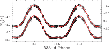
Fig. 1 shows the Hα equivalent-width measurements, which vary between +1.4 and −4.3 Å, folded on the adopted ephemeris; it illustrates a number of noteworthy points.
![Hα measurements folded on the ephemeris of equation (2), shown over two cycles. Upper panel: equivalent-width [the solid line is the ad hoc functional fit, equation (1), described in Section 3.1]. Middle panel: FWHM (upper groups of points) and central velocity (lower) of excess emission. Bottom panel: the Hipparcos photometry (with a scaled, vertically shifted version of the Hα functional fit to guide the eye).](https://oup.silverchair-cdn.com/oup/backfile/Content_public/Journal/mnras/381/2/10.1111_j.1365-2966.2007.12178.x/4/m_mnras_381_2_433_f1.jpeg?Expires=1750373420&Signature=a-AkmtazyWTL5av88u05EfuVJM8lctrzjGVPmF6cOx7tlmrpiR3RMnk8EVnA-Ap6NRccMS7zgNs-z7LXIkuyrFcRMmzK3kLEI-nA~ORrewsbNB2LXD-jOqG9Zhg7dDnh2PWVI~61smvDlM-4R8S66v8E-JvVkkJzGvXFiaKfawSVY9c1wflbwKfP8qqHdBCiuX97t85iIMDbytKOwNR-5ttyaxt~vNhD6ypfaxMhDP5srE86MXV6dokwdNjkfcEYF4vIv5ofxiNtoL2RhakrZDZ~nWc2FzT-NCDT-vcswiJGW8rLXIbfBWj~46lGyy3WkdJe-wyIiMrmcTLgmmylrg__&Key-Pair-Id=APKAIE5G5CRDK6RD3PGA)
Hα measurements folded on the ephemeris of equation (2), shown over two cycles. Upper panel: equivalent-width [the solid line is the ad hoc functional fit, equation (1), described in Section 3.1]. Middle panel: FWHM (upper groups of points) and central velocity (lower) of excess emission. Bottom panel: the Hipparcos photometry (with a scaled, vertically shifted version of the Hα functional fit to guide the eye).
The Hα light curve is remarkably symmetrical about phase zero.
There is a well-defined interval of apparent ‘quiescence’, lasting ∼0.3 (=1–2φ0) of the period.
The behaviour is repeatable from the earliest quantitative data (1982),4 supporting a truly periodic underlying 538-d ‘clock’.
None the less, the Hα profiles are evidently not strictly repeatable; the standard deviation of Wλ measurements about the functional fit is only 0.16 Å, but scrutiny of the spectra shows that real, small-amplitude variability contributes to this dispersion at all sufficiently well-sampled phases, including quiescence, on time-scales longer than a few days. We suspect that any O-type star observed as extensively and intensively as HD 191612 may show Hα‘jitter’ at a similar level (cf., e.g., Kaper et al. 1997; Morel et al. 2004).
The Hα profile during quiescence is asymmetric and filled in by stellar-wind emission (Fig. 2). It is intermediate in appearance between the profiles of HD 36861 [λ Ori; O8 III((f)), pure absorption] and HD 175754 [O8 II((f)), P Cygni], although the closest matches among the spectra at our disposal are with HD 193514 [O7 Ib(f)] and HD 209975 [O9.5 Ib; Fig. 2].5 Thus while we have no exact match to the quiescent spectrum, the Hα profile in that state seems to be largely unremarkable, with no evidence of substantial excess emission relative to normal stars of broadly comparable spectral type.
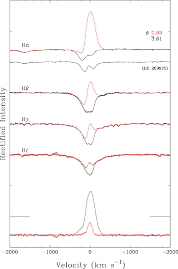
Balmer-line profiles for HD 191612 at quiescence ( , in black) and near emission maximum (φ= 0.89, red); the tickmarks on the y-axis are separated by half the continuum level. The Hα spectrum of HD 209975 is included to demonstrate that a near match to the minimum-state spectrum can be found among normal stars (see Section 3.2 for details). Difference spectra for Hα and Hζ are shown at the bottom of the plot. Velocities are heliocentric.
At other phases, the line-profile morphology is P Cygni like, but the increase in emission is not necessarily associated with an increase in the global mass-loss rate (cf. Section 4.2). Phenomenologically, the changes in the appearance of the profile can be entirely accounted for by variable amounts of roughly Gaussian emission superimposed on a constant, underlying quiescent-state spectrum (Fig. 2). We have characterized the mean velocity displacement and width of this excess emission by Gaussian fits; results are incorporated in Fig. 1. Significant phase dependence is evident for neither mean velocity nor full width at half-maximum (FWHM), which average +7 and 271 km s−1, respectively (standard deviations of 10 and 16 km s−1, commensurate with likely observational uncertainties); the width of the excess emission is much less than both the stellar-wind terminal velocity (Section 6.4), and the ‘windy’ Hα emission normally seen in luminous O stars.
Finally, although the Hα and Hipparcos light curves are in phase (to within the errors), we note that the photometric variations are too large to result from excess line emission alone; most of the ∼3–4 per cent change must arise from true continuum-level variations.
4 THE 538-D PERIOD: OTHER VARIABLE LINES
4.1 Balmer and He i lines
Other Balmer lines (to at least H10)6 and the He i lines all show large variations, in both strength and velocity, which are reproducible on the 538-d period. He i 4471 Å (Fig. 3) exemplifies the typical behaviour of the He i lines; most remain in absorption at all phases, although He iλλ5876, 7065, 7281, as well as Hα and Hβ, show strong P-Cygni-like emission at maximum. While most lines are in absorption during quiescent phases (even Hα, as illustrated with other Balmer lines in Fig. 2), He i 6678 Å is exceptional in retaining an emission core (Fig. 4).
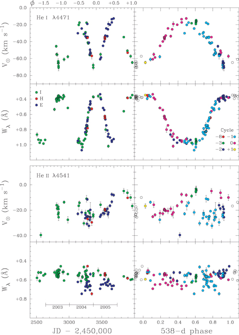
Equivalent-width and velocity variations for He i 4471 Å and He ii 4541 Å. Points with large formal measurement errors are omitted for clarity (so that fewer velocities than line strengths are plotted). As in Fig. 1, the equivalent-width axis is inverted (such that lower points indicate greater absorption/less emission). The points in the left-hand panels are colour-coded according to the source: E(lodie; Nazé et al. 2007), H(igh-resolution), or I(ntermediate-dispersion). The points in the right-hand panels are colour-coded according to the cycle in the ephemeris of equation (2).
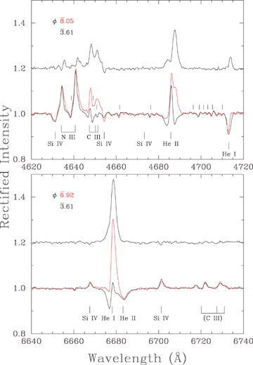
Emission-line variability in HD 191612; spectra are labelled by phase in the Hα ephemeris of equation (2). Data obtained near Hα maximum are shown in red; those near minimum in black; ratio spectra are shown offset by +0.2. (All spectra were obtained near orbital zero; Section 5.3.) Upper panel: the N iii 4640 Å, C iii 4650 Å, He ii 4686 Å emission-line complex; the unlabelled tick marks indicate wavelengths of O ii lines. Note also the infilling of the red wing of He i 4713 Å. Lower panel: He i/He ii 6678/6681 Å. Although λ6678 is unusual among the He i lines in showing emission throughout ‘quiescence’, the qualitative nature of the variability (i.e. growth of a slightly redshifted, fairly narrow emission superimposed on the quiescent-state spectrum) is notable only for the unusually large relative amplitude. The λλ6717/6722/6729 lines (the latter probably a blend in our data, λ6728.8+6731.1:) are almost constant in strength; the positions appear not to be consistent with a standard C iii identification.
The basic phenomenology of the variability is, evidently, infilling of a near-normal underlying absorption profile by slightly (∼20–30 km s−1) redshifted, almost symmetrical emission (cf. Fig. 2). This interpretation is consistent both with direct inspection of line profiles and with the phase dependence of variability; all lines share a common velocity around φα≃ 0.5, becoming increasingly blueshifted with decreasing line strength (i.e., increasing emission infill). Moreover, the amplitude of radial velocity variation correlates with the amplitude of line-strength variation.
This phenomenology appears to be applicable to almost all variable features, embracing not only the hydrogen and He i lines (including λ6678), but also the signature Of?p C iii 4650 Å transitions (Fig. 4; the adjacent N iii lines are much less, if at all, variable, and so are evidently dominated by ‘normal’, photospheric, Of emission). He iiλ4686 shows an exceptional pattern of variability; narrow emission is present even at quiescent phases, and while the overall emission-line strength increases near phase zero, only small changes occur at the position of this narrow emission (Fig. 4), possibly because the emission is already optically thick here.
4.2 Ultraviolet P-Cygni profiles
Walborn et al. (2003) presented a high-resolution International Ultraviolet Explorer (IUE) spectrum obtained on 1992 December 19 (JD 244 8975.9,  Å). There are no other high-dispersion ultraviolet (UV) spectra available, but the IUE archive contains a low-resolution, short-wavelength spectrum (1984 July 25, JD 244 5907.0,
  ). After smoothing and binning the high-resolution spectrum to render it comparable to the low-resolution one (Fig. 5), there is no evidence for large changes in the resonance-line profiles of N vλ1240, Si ivλ1400 and C ivλ1550 (although we cannot rule out variations at the moderate level observed in the oblique rotator θ1 Ori C; Walborn & Nichols 1994). This encourages the view that the Hα variability results from the changing visibility of a constrained plasma, rather than a large-scale global change in outflow characteristics – for example, if the variability were a consequence of changes in mass-loss rate, this would be expected to have a clear signature in the UV P-Cygni profiles.
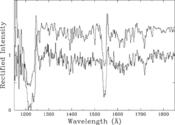
IUE spectra of HD 191612. Lower spectrum: low-resolution,  ; upper spectrum (offset by 0.5 continuum units): high-resolution spectrum,
  , smoothed and binned to match the low-resolution data.
5 THE CONSTANT LINES
In contrast to the hydrogen and He i lines, the absorption lines of metals and of He ii, together with many selective emission lines, show only small changes, at most, in line strength. For simplicity, we label such lines as ‘constant’; if there is any line-strength variability, it is at a very low level.
5.1 Absorption lines
The C iv 5801, 5812 Å doublet exemplifies the behaviour of the constant absorption lines. This doublet is particularly well suited to measurement both on astrophysical grounds (the lines are very symmetrical, and are formed deep in the atmosphere, and hence are less likely to be contaminated by ‘windy’ emission than many other transitions (cf., e.g., Fullerton, Gies & Bolton 1996), and observationally (the nearby diffuse interstellar bands at 5778/5780/5797 Å are of similar strength to the C iv lines, and provide a very useful zero-point calibration for the wavelength scale, allowing rather precise differential velocities to be obtained even from intermediate-dispersion data of unexceptional quality).
The C iv measurements are presented in Fig. 6, and illustrate the typical behaviour of essentially constant line strength coupled with small-amplitude radial-velocity variations. The steady increase in velocity between JDs ∼245 3500 and 245 3700 discussed by Nazé et al. (2007) clearly does not repeat on the 538-d period. Metal absorption lines strong enough to be measured consistently in most spectra (e.g. N iiiλλ4511–4534), as well as the He ii absorption lines (e.g. λλ4200, 4541, 5411), follow essentially the same behaviour as the archetypal C iv lines, as illustrated in Fig. 3 by data for He iiλ4541.
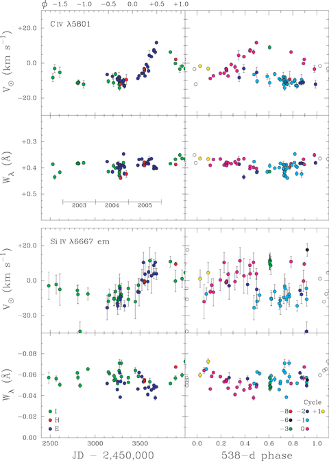
Equivalent-width and velocity variations for the C iv 5801 Å absorption and Si iv 6667 Å emission lines; other details are as for Fig. 3.
5.2 Selective emission lines
The high-quality UES and CFHT spectra, in particular, reveal a rich spectrum of selective emission lines (cf. Walborn 2001). In general, the weakness of the lines precludes detailed scrutiny of their phase dependence in the remaining data, but comparison of quiescent and emission-line phases in these echellograms establishes that most of the emission features7 exhibit essentially the same behaviour as the C iv lines (i.e., near-constant line strength and small-amplitude radial velocity variations). Only the stronger lines can be consistently measured, but results for Si iv 6667 Å shown in Fig. 6 illustrate the general accord between the behaviours of the selective emissions and the ‘constant’ absorption lines.
The extensive far-red coverage of the high-quality CFHT ESPaDOnS spectra allows many other weak emission lines to be recognized; these appear also to show little or no variability in line strength (at least, between the two epochs sampled, at 538-d phases 0.24 and 0.89; the ‘variable’ lines discussed in Section 4 change substantially between these epochs). Most of these features are previously unreported in O star spectra, and currently lack persuasive identifications. Measured wavelengths in Å[and possible identifications, with multiplet numbers from Moore (1945)] are, for the stronger features, 5739.8; 6394.8, 6467.1, 6478.7 (N iii 14? good wavelength matches but not all multiplet members present); 6482.3; 7002.8; 7037.2 (C iii 6.01); 7306.9; 7455.2; 7515.7; 8019.2 (N iii 26); 8103.0 (Si iii 37); 8196.6 (C iii 43); 8251.0; 8265.7; 8268.9; 8286.8; and 9705.5, 9715.4 (each strong and broad; C iii 2.01).
5.3 Radial-velocity variations and spectroscopic orbit
The ‘constant’ lines show significant, systematic radial-velocity variations8 which do not repeat with the 538-d period (Figs 3 and 6; Table A2). These velocity variations cannot reflect photospheric motion about a static centre of mass (the implied change in radius is as great as ∼250 R⊙, or ∼17R*). In principle, they could be attributed to changes in the depth of line formation in an accelerating outflow, through density changes in or near the transonic region resulting from stochastic changes in the stellar-wind mass-loss rate. However, the lack of changes in Hα in mean quiescent spectra around phases  and 0.5 (corresponding to negative- and positive-velocity C iv states) does not encourage confidence in this interpretation, and we have already argued that the C iv lines are formed relatively deep in the subsonic atmosphere.
Velocities used in orbital solutions. Note that each of the three data sets is subject to a separate velocity zero-point error of the order of a few km s−1 (see footnote 9).
| JD | V⊙ (km s−1) | JD | V⊙ (km s−1) | JD | V⊙ (km s−1) | JD | V⊙ (km s−1) | JD | V⊙ (km s−1) |
| C iv 5800 Å | |||||||||
| 244 9529.4 | −9.3 | 245 3203.5 | −11.3 | 245 3275.2 | −11.3 | 245 3474.6 | −8.8 | 245 3601.4 | +4.4 |
| 245 2127.5 | +9.0 | 245 3225.8 | −6.3 | 245 3276.2 | −10.6 | 245 3488.6 | −7.3 | 245 3625.4 | +3.7 |
| 245 2528.8 | −8.3 | 245 3246.3 | −8.9 | 245 3278.3 | −11.7 | 245 3519.6 | −5.9 | 245 3652.3 | +7.0 |
| 245 2549.4 | −3.1 | 245 3251.3 | −9.6 | 245 3282.4 | −12.0 | 245 3536.7 | −5.8 | 245 3653.3 | +7.6 |
| 245 2607.3 | −5.3 | 245 3264.3 | −7.8 | 245 3283.3 | −10.1 | 245 3545.0 | −3.2 | 245 3668.3 | +6.3 |
| 245 2801.6 | −11.4 | 245 3265.3 | −9.6 | 245 3302.3 | −11.3 | 245 3546.0 | −3.7 | 245 3681.3 | +11.7 |
| 245 2808.5 | −11.2 | 245 3266.3 | −12.2 | 245 3314.6 | −10.3 | 245 3547.0 | −3.5 | 245 3836.8 | +6.3 |
| 245 2816.6 | −11.0 | 245 3267.2 | −9.9 | 245 3316.3 | −9.7 | 245 3548.0 | −4.3 | 245 3892.7 | −0.2 |
| 245 2871.2 | −12.1 | 245 3267.4 | −8.2 | 245 3320.3 | −12.9 | 245 3554.6 | −7.4 | 245 3896.0 | +2.1 |
| 245 3132.9 | −6.5 | 245 3269.2 | −10.9 | 245 3324.3 | −12.7 | 245 3568.5 | −0.8 | 245 3941.5 | −3.4 |
| 245 3146.7 | −10.4 | 245 3270.2 | −14.2 | 245 3326.3 | −13.2 | 245 3585.5 | −2.2 | 245 3966.6 | −1.7 |
| 245 3192.5 | −7.6 | 245 3272.4 | −8.3 | 245 3346.4 | −9.5 | 245 3594.5 | −4.5 | 245 4002.5 | −3.2 |
| λ6700 emission | |||||||||
| 245 0683.5 | −9.4 | 245 2808.5 | −34.8 | 245 3266.6 | −36.6 | 245 3474.6 | −33.3 | 245 3594.5 | −22.0 |
| 245 2127.4 | −16.4 | 245 2919.3 | −34.6 | 245 3270.2 | −30.2 | 245 3480.7 | −29.6 | 245 3607.4 | −15.6 |
| 245 2128.4 | −16.2 | 245 3132.9 | −42.5 | 245 3272.4 | −31.4 | 245 3488.6 | −33.6 | 245 3625.4 | −24.2 |
| 245 2129.4 | −17.6 | 245 3146.7 | −38.8 | 245 3278.3 | −37.8 | 245 3519.6 | −26.6 | 245 3652.3 | −18.2 |
| 245 2129.6 | −15.3 | 245 3157.7 | −35.3 | 245 3283.3 | −36.0 | 245 3536.7 | −16.6 | 245 3653.3 | −23.1 |
| 245 2130.4 | −15.6 | 245 3209.7 | −37.2 | 245 3290.6 | −34.7 | 245 3545.0 | −28.0 | 245 3668.3 | −16.5 |
| 245 2132.7 | −18.3 | 245 3210.5 | −37.6 | 245 3291.6 | −36.2 | 245 3546.0 | −28.0 | 245 3681.3 | −23.1 |
| 245 2483.6 | −29.9 | 245 3225.8 | −33.2 | 245 3326.3 | −41.4 | 245 3547.0 | −27.8 | 245 3836.8 | −16.1 |
| 245 2566.3 | −29.2 | 245 3246.3 | −40.0 | 245 3368.3 | −31.4 | 245 3548.0 | −27.2 | 245 3892.7 | −27.2 |
| 245 2607.3 | −32.0 | 245 3250.5 | −38.2 | 245 3369.3 | −37.7 | 245 3554.6 | −23.3 | 245 3896.0 | −17.5 |
| 245 2801.6 | −32.6 | 245 3251.3 | −41.5 | 245 3446.7 | −39.0 | 245 3585.5 | −27.5 | 245 3966.6 | −25.8 |
| O iiabsorption | |||||||||
| 245 2101.6 | −28.7 | 245 2566.3 | −24.6 | 245 3157.7 | +21.6 | 245 3266.6 | +19.7 | 245 3681.3 | −35.1 |
| 245 2127.4 | −33.0 | 245 2632.3 | −5.9 | 245 3209.7 | +15.7 | 245 3554.6 | −6.6 | 245 3836.8 | −32.7 |
| 245 2127.5 | −33.5 | 245 2808.5 | +7.2 | 245 3210.5 | +6.9 | 245 3568.5 | −11.1 | 245 3892.7 | −21.4 |
| 245 2128.4 | −33.4 | 245 2816.6 | +5.7 | 245 3225.8 | +11.3 | 245 3625.4 | −26.3 | 245 3896.0 | −23.4 |
| 245 2129.4 | −32.7 | 245 2831.6 | +6.1 | 245 3246.3 | +5.0 | 245 3652.3 | −19.1 | 245 3941.5 | −17.2 |
| 245 2130.4 | −34.9 | 245 2837.6 | +14.3 | 245 3250.5 | +11.6 | 245 3653.3 | −25.8 | 245 3966.6 | −20.4 |
We therefore consider the possibility of orbital motion on periods other than that of the major spectroscopic variability. We concentrate on measurements of the C iv 5800 Å doublet and the ∼6700 Å emission-line complex (Si iv+ unidentified), which yield mutually consistent results. Both features have velocity zero-points tied in to nearby, moderately strong Diffuse Interstellar Bands (we adopted DIB wavelengths as measured in the CFHT spectra), and therefore record the velocity variations more precisely and accurately than other lines that lack this advantage. Results are given in Table A2.
Fortuitously, the data set includes good-quality observations showing that relatively large positive velocities occurred in 538-d cycles −3 and −6, as well as at φα∼ 0.5, hinting at Porb≃ 3Pα. Trial orbital solutions with Porb≃ 1500–1600 d yielded residuals that are satisfactorily small, but none the less slightly larger than the formal errors returned by the Gaussian fits to lines used to measure velocities. Since external errors evidently dominate (C iv) or match (Si iv) the formal uncertainties, we weighted all C iv measurements and all Si iv measurements equally, but with the Si iv measurements assigned approximately one-third weight to reflect their greater residuals (and adjusted by −2.1 km s−1 to bring them to the same γ velocity as the C iv measurements).
The resulting orbital solution is summarized in Table 2, and illustrated in Fig. 7. While this solution has not yet been subject to the acid test of predictive power, its success in reproducing observations at three separate periastron passages, with small residuals that are consistent with realistic observational uncertainties, encourages the view that the solution does characterize a true binary orbit.
Orbital solution. The main orbital parameters are constrained by measurements of C iv 5801 Å and Si iv 6667 Å in the primary spectrum; K2 is established from O ii lines in the secondary spectrum.
| γ | −5.19 | ± | 0.36 | km s−1 |
| K1 | 11.77 | ± | 0.84 | km s−1 |
| e | 0.438 | ± | 0.038 | |
| ω |  | ± |  | |
| Porb | 1542 | ± | 14 | d |
| T0 | JD 245 3720 | 20 | ||
| f(m) | 0.190 | ± | 0.042 | M⊙ |
| a1 sin i | 322 | ± | 24 | R⊙ |
| rms residual | (weight 1, C iv) 2.2 km s−1 | |||
| K2 | 24.4 | ± | 1.4 | km s−1 |
| f(m) | 1.68 | ± | 0.29 | M⊙ |
| a2 sin i | 667 | ± | 38 | R⊙ |
| q=M2/M1 | 0.483 | ± | 0.044 | |
| rms residual | (O ii) 5.1 km s−1 | |||
| γ | −5.19 | ± | 0.36 | km s−1 |
| K1 | 11.77 | ± | 0.84 | km s−1 |
| e | 0.438 | ± | 0.038 | |
| ω | | ± | | |
| Porb | 1542 | ± | 14 | d |
| T0 | JD 245 3720 | 20 | ||
| f(m) | 0.190 | ± | 0.042 | M⊙ |
| a1 sin i | 322 | ± | 24 | R⊙ |
| rms residual | (weight 1, C iv) 2.2 km s−1 | |||
| K2 | 24.4 | ± | 1.4 | km s−1 |
| f(m) | 1.68 | ± | 0.29 | M⊙ |
| a2 sin i | 667 | ± | 38 | R⊙ |
| q=M2/M1 | 0.483 | ± | 0.044 | |
| rms residual | (O ii) 5.1 km s−1 | |||
Orbital solution. The main orbital parameters are constrained by measurements of C iv 5801 Å and Si iv 6667 Å in the primary spectrum; K2 is established from O ii lines in the secondary spectrum.
| γ | −5.19 | ± | 0.36 | km s−1 |
| K1 | 11.77 | ± | 0.84 | km s−1 |
| e | 0.438 | ± | 0.038 | |
| ω | | ± | | |
| Porb | 1542 | ± | 14 | d |
| T0 | JD 245 3720 | 20 | ||
| f(m) | 0.190 | ± | 0.042 | M⊙ |
| a1 sin i | 322 | ± | 24 | R⊙ |
| rms residual | (weight 1, C iv) 2.2 km s−1 | |||
| K2 | 24.4 | ± | 1.4 | km s−1 |
| f(m) | 1.68 | ± | 0.29 | M⊙ |
| a2 sin i | 667 | ± | 38 | R⊙ |
| q=M2/M1 | 0.483 | ± | 0.044 | |
| rms residual | (O ii) 5.1 km s−1 | |||
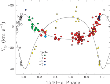
Radial-velocity measurements for C iv 5801 Å (large circles), Si iv 6667 Å (diamonds), and O ii lines (small yellow circles), plotted with the orbital solution of Table 2. The C iv and Si iv points are colour-coded according to cycle count in the ephemeris of Table 2, and for display purposes the O ii velocities have been adjusted by −14.3 km s−1 to bring them to the same γ velocity as the primary (see footnote 9).
5.3.1 Secondary orbit
A careful examination of weak lines of low-ionization stages in the best data shows velocity displacements in antiphase with the stronger lines, bolstering the interpretation of the 1540-d velocity variations as being orbital in origin. The spectroscopic fingerprint of the secondary is weak, but its velocity can be reasonably well quantified by simultaneous Gaussian fits to a selection of a half-dozen unblended, relatively strong O ii absorption lines (λλ4300–4700 Å, central depths 2–3 per cent below continuum), constrained to share the same velocity shift; results are included in Table A2.
Although we do not have the benefit of well-defined interstellar features to provide a velocity reference for most observations encompassing the O ii-line spectral region, we can exploit the fact that the centrally placed He ii 4541 Å line follows the motion of the C iv and Si iv features used to determine the primary's orbit (Section 5.1). By measuring O ii velocity differences with respect to λ4541, and correcting for computed motion of the primary, we can in effect remove spectrum-to-spectrum velocity zero-point offsets. (Using directly observed velocities gives essentially identical results, but with somewhat larger scatter.)
An orbital solution of the resulting O ii velocities gives γ and K2 (with all other parameters fixed at the primary-orbit values9); the slope of He ii versus He ii–O ii velocities gives an entirely consistent mass ratio. Results are incorporated into Table 2.
5.3.2 Relationship between the 538- and 1540-d periods?
The orbital period is ∼3 × 538 d, which has suggested to colleagues the possibility of some sort of resonance. However, a solution with Porb≡ 3Pα gives a significantly poorer fit than one with Porb allowed as a free parameter.10 Thus, although it seems to be quite securely established that HD 191612 is a long-period binary, it appears that, with Porb= 2.87 ± 0.03Pα, the binary orbit has no direct important role in the large-amplitude spectroscopic variability.
There is, however, an interplay between the periods in a limited observational sense, explaining otherwise complex behaviour seen in some lines. Fig. 8 shows spectra obtained near the extremes of both the orbital motion and the spectroscopic variability. In addition to illustrating the small orbital velocity amplitudes (less than the linewidths) the quiescent-state spectra clearly indicate that absorption in the Si iiiλλ4552, 4568, 4575 triplet tracks the secondary spectrum, on the orbital period. The primary spectrum has emission in these lines which varies on the 538-d period, and which shows a strong decline in strength going from λ4552 to λ4575 (as is observed in some LBV/WN11 spectra; e.g. He 3-519, Walborn & Fitzpatrick 2000).
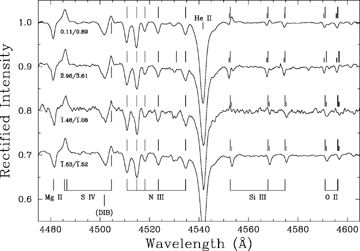
Signatures of the secondary's spectrum. Data have been lightly smoothed, rebinned, and renormalized to facilitate comparison between observations, which are labelled by orbital/Hα phases (Section 5.3/3.1). Spectra have been shifted to bring the primary to zero velocity; the long tick marks indicate rest wavelengths of the identified lines. In this reference frame, the He ii, N iii and S iv lines show no significant movement (i.e., arise principally in the primary's spectrum). The short tick marks show the expected positions of the O ii and Si iii lines in the secondary spectrum, according to the orbital solution given in Table 2.
The interplay of these two cycles means that the lines can appear purely in absorption (throughout quiescent 538-d phases), but in other states the behaviour is more complex. When the primary and secondary spectra are at or near maximum velocity separation, a P-Cygni-like appearance results in λλ4552, 4568, with absorption in λ4575 (as in the first [top] spectrum in Fig. 8); emission phases at smaller velocity separations can result in apparent disappearance, or nulling, of λ4552 (third spectrum in Fig. 8).
A similar effect is detectable in the N ii spectrum, in particular the 5001/5005 Å lines, where primary emission and secondary absorption clearly move in antiphase; and, possibly, in the λλ4414.9, 4417.0 O ii lines.
5.4 System characteristics
Mass constraints implied by the orbital solution are illustrated in Fig. 9. We have no constraint on the orbital inclination, but the masses are entirely consistent with a system comprising a ∼30 M⊙, late-O giant accompanied by a ∼15 M⊙, early-B main-sequence star, viewed at an intermediate angle (sin i≃ 0.5). The projected centres-of-mass separation at periastron is (1–e)a sin i= (555 ± 68) R⊙ (∼40R*); although this certainly allows for the possibility of wind–wind interactions, the dominant Hα emission region, for example, is surely much closer to the primary, so that it is unlikely that the secondary plays any important role in the 538-d changes.
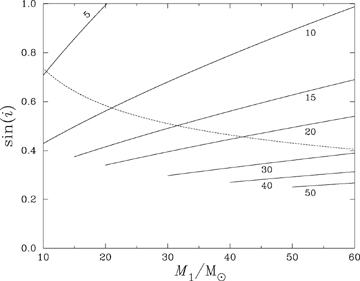
Constraints on the system mass resulting from the orbital solution of Table 2. The solid lines are loci of constant secondary mass, labelled in solar masses, implied by the mass function (assuming M2≤M1); the dotted line shows the estimated mass ratio.
The strong variability of the He i classification lines, together with the small orbital-velocity amplitudes (which ensure that the components' helium lines are never resolved in the spectrum) means we cannot estimate the spectral types separately from the spectrum; the maximum velocity separation is less than the linewidths in the primary. Thus, even if the components were as just postulated, with an expected B-band brightness ratio of ∼10:1, the combination of the likely differences in spectral types and the resolution and S/N of most of our spectra means that it is not particularly surprising that we do not see truly double-lined features (other than the peculiar Si iii lines noted in Section 5.3.2). None the less the O ii/Si iii lines indicate a secondary spectral type not earlier than B0, and not later than B2 (assuming a dwarf luminosity class and normal composition).
6 OTHER SPECTROSCOPIC PROPERTIES
6.1 Spectral classification
Our extended data set, and improved understanding of the spectroscopic variability, allow us to revisit the spectral classification (i.e., the classification of the spectrum– not the component stars).
The φα= 0 spectrum (specifically, the WHT spectrum of JD 245 3941.5) yields spectral type O6.5f?pe (‘O6.5’ from the He i 4471/He ii 4541 ratio, with qualifiers ‘f?p’ from C iiiλ4650 and ‘e’ from the Hγ emission). Our refined classification of the quiescent-state spectra is O8fp (the weakness of C iii in that state excluding Of?p). Of course, it is now clear that this apparent variability in spectral type does not reflect changes in any fundamental stellar properties – which would result in large-amplitude photometric variability – but instead results from infilling of the He iλ4471 classification line by emission.
These results are in full accord with previous classifications, including in particular Walborn's (1973) original blue-region spectrum, obtained on 1972 September 24  and also classified O6.5f?pe (Walborn 1973) – consistent with the underlying ‘clock’ keeping good time for at least a decade before the earliest digital data.
A luminosity classification at any state is not possible because of the unique, peculiar profile of the fundamental He ii 4686 Å criterion. The strength of Si iv 4089 Å relative to nearby He i lines would be consistent with luminosity class V, while the UV Si iv resonance doublet is neither dwarf- nor supergiant-like, but is possibly consistent with class III. The physical properties established in Section 6.3 are also broadly giant-like. However, all the known Of?p stars are sufficiently spectroscopically peculiar that any luminosity-class argument based on direct comparisons with normal stars must be considered hazardous.
6.2 Spectroscopic fine analysis
Although the peculiarities of the spectra preclude extremely detailed modelling, the basic photospheric parameters can none the less be quite well constrained. We searched for matches to the ‘quiescent’ spectrum of 2001 August 5  , in a grid of fastwind models (Puls et al. 2005) sampled at steps of 1 kK and 0.2 in Teff and log g (with Y= 0.1 and vturb= 15 km s−1). We find a generally good match with observations for a model with Teff= 35.0 kK, log g= 3.5, in excellent agreement with the analysis reported by Walborn et al. (2003, based on simpler models and poorer-quality data).
No model reproduces the strength of He i 4471 Å (cf. the general discussion of this issue by Repolust, Puls & Herrero 2004), but the He i singlet lines are fully consistent with the estimated Teff; adopting 34 kK would still require log g= 3.5, but leads to the model He ii lines becoming too weak. The best-fitting model parameters can therefore be considered as fairly well determined, to ∼±1 kK, 0.1 in Teff, log g (although, of course, no model matches the peculiar He ii 4686 and He i 6678 Å profiles).
This takes no account of the effect of the secondary spectrum, which is expected to have somewhat stronger He i lines, while the He ii line strengths may be underestimated by ∼10 per cent through dilution. This would result in the primary being, if anything, modestly warmer (by perhaps ∼1 kK) than the foregoing analysis suggests.
6.3 Reddening, radius
To determine the reddening and angular diameter, we compared a Teff= 35.0 kK, log g= 3.5Ostar2002 model (Lanz & Hubeny 2003) with archival low-resolution IUE spectrophotometry and optical & 2MASS photometry (Flux variability is of too small an amplitude to be of oncern here). We estimate (Reff/R⊙)/(D/kpc) = 6.7 ± 0.05 and E(B−V) = 0.56 ± 0.03[using a Cardelli, Clayton & Mathis 1989 reddening law with RV≡AV/E(B−V) = 3.1], where Reff is an ‘effective’ radius characterizing the emitting surfaces. The match between the model and observations, though not perfect, is reasonably good, and there is no evidence of any infrared excess out to 2μm. The fit is slightly improved by allowing for the contribution of a cooler secondary, such as a ∼20 kK secondary contributing ∼10 per cent of the light at V, and this ad hoc model is illustrated in Fig. 10.
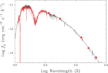
Spectral energy distribution for HD 191612 (red). The weighted sum of an Ostar2002 model with Teff= 35 kK, log g= 3.5 and an Atlas9 model with Teff= 20 kK, log g= 4.5, with a V-band flux ratio of 9:1 and E(B−V) = 0.56, is shown for comparison (black; see Section 6.3 for details).
6.4 Hα mass-loss rate
 dex M⊙ yr−1. As for other aspects of the fastwind analysis, this is in satisfactory agreement with the corresponding result reported by Walborn et al. (2003;
  =−5.6 dex M⊙ yr−1).
6.5 Rotation
The equatorial velocity expected for a 538-d rotation period and R*≃ 14.5 R⊙ is ∼1.4 km s−1, and a measurement of ve sin i would provide a strong test of rotational modulation. (For reference, the equatorial rotation velocity for synchronous rotation is ∼0.5 km s−1, or, for pseudo-synchronous [periastron-synchronized] rotation, ∼0.8 km s−1.) Most lines in the spectrum show asymmetries or variability to some extent but, as already discussed, the C iv 5800 Å doublet shows exceptionally symmetrical profiles with little or no evidence of contamination by emission; these high-excitation lines are expected to form rather deep in the atmosphere, and therefore to be more representative of the subsonic photosphere than many other features.
Donati et al. (2006a; see also Howarth 2003) showed that the C iv profiles deviate strongly from those expected from rotational broadening, but are well matched by simple Gaussian ‘turbulence’, with zero rotation. We have attempted to set upper limits to the rotation rate by looking for zero-amplitude nodes in the Fourier transform of the profiles (Gray 1992) in the combined 2005 CFHT spectra (S/N > 103). We compared the results with transforms of synthetic spectra that include rotational broadening, isotropic Gaussian macroturbulence, and Gaussian noise, using an intrinsic profile from an Ostar2002 model (Lanz & Hubeny 2003).
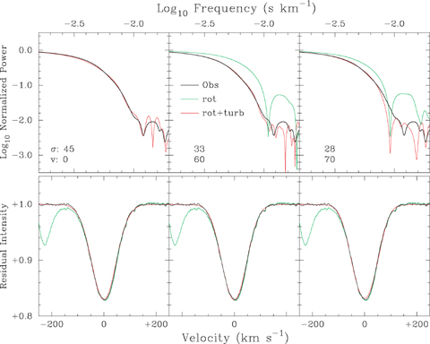
Illustrative line-broadening models for the C iv 5801 Å line. Upper panels: results in the Fourier domain. The solid black lines show the transform of the observed profile (i.e.. the transform of the black spectrum in the lower panels); the red lines show the transforms of synthetic profiles computed with isotropic Gaussian macroturbulence (with dispersion σ, in km s−1), rotational broadening (with ve sin i=v), and Gaussian noise; and the green lines show the transforms for rotational broadening alone. Any model with ve sin i≲ 60 km s−1 (and appropriate macroturbulence) is acceptable. Lower panels: results in the wavelength domain. The observed spectrum is shown in each panel in green (the directly observed profile) and black (the version of the profile used in the analysis, after re-rectification to take out the diffuse interstellar band). The synthetic profiles, shown in red, are the inverse transforms of the models shown in red in the upper panels. At this scale, the synthetic profiles (which have been modestly scaled in intensity to match the observed line strength) are almost indistinguishable from each other, and from the observed spectrum, in the wavelength domain.
7 DISCUSSION
The symmetry and reproducibility of, in particular, the Hα 538-d light curve strongly suggest an origin in an essentially geometrical process – that is, the changing aspect of a distinct emission region. This is also consistent with the absence of evidence of associated global changes in stellar-wind properties (Section 4.2). Since we have found that the variability is not orbital, our results lend strong support to the proposal by Donati et al. (2006a) of rotationally modulated line emission from a magnetically constrained plasma.
One might hope that the fairly rich emission spectrum would offer insight into physical conditions in the line-forming region, but there is a dearth of traditional nebular diagnostics (suggesting a high-density regime). We can only infer some general characteristics of the Hα-emitting region. First, optically thin Hα emission in any time-independent axisymmetric structure cannot account for the observed 538-d behaviour; at least half the emission from any such structure would visible at all times, but emission equivalent to the adopted ‘excess’ emission cannot plausibly be present during ‘quiescent’ phases. At the same time, very complex geometries (such as observed in τ Sco; Donati et al. 2006b) are unlikely, as they would not be consistent with the large amplitude of emission variability.
If we adopt the hypothesis that the geometry of the line-emitting region is determined by the magnetic field, then the simplest acceptable magnetic field geometry is a misaligned, centred dipole – known to provide a reasonable approximation to θ1 Ori C, the prototype magnetic O star (Stahl et al. 1996; Donati et al. 2002; Wade et al. 2006). Babel & Montmerle (1997) argue that, for such a geometry, stellar-wind material from the magnetic polar and temperate regions will be deflected along the field lines towards the magnetic equator, where the colliding flows shock to create a high-temperature, X-ray-emitting plasma. The plasma cools to form a dense disc which gives rise to optical emission. Magnetohydrodynamic calculations support this general outline, albeit with a number of refinements (e.g. ud-Doula & Owocki 2002; Gagné et al. 2005; Ud-doula, Townsend & Owocki 2006).
Since this model is at least consistent with the direct magnetic field measurements of HD 191612 (Donati et al. (2006a), for heuristic purposes we explore schematic ‘toy’ models of Hα emission from a centred, tilted, geometrically thin disc, in which the relative emission is simply related to the projected area (taking into account limb darkening and occultation by the star). Although this is a physics-free, geometrical model, we can speculate that it may characterize a more realistic scenario; for example, for a disc-like emission region, the ‘limb darkening’ may actually correspond to increasing Hα optical depth as the line of sight approaches the plane of the disc.
We find that this simple model can provide a reasonable match to the Hα variability, provided that (i) the sum of the inclination of the rotational axis to the line of sight and the angle between that axis and the magnetic axis is close to 90°, and (ii) moderately strong limb-darkening is present (so that the emission is low at all rotational phases when the line of sight is close to the disc plane). Moreover, the width-to-thickness ratio must be reasonably large, to account for the large amplitude of emission-line variability.
A specific model, selected through a genetic-algorithm minimization, is shown in Fig. 12; its parameters are inner radius Rin= 2.00R*, outer radius Rout= 2.13R*, axial inclination i= 68°, magnetic-axis offset α= 27°, and linear limb-darkening coefficient u= 0.7. These parameters should be regarded only as illustrative, as many other combinations give closely similar fits (e.g. 1.55R*, 1.76R*, 41°, 56°, 0.6 gives results almost indistinguishable from those in Fig. 12). The radii, in particular, are only very weakly constrained from the Hα light curve, because the total emission is fixed by an arbitrary scaling factor (parametrizing the surface emissivity).
‘Toy’ models compared to phased Hα equivalent widths (circles). Lower model (left-hand axis): a single surface ‘spot’; upper model (right-hand axis): an optically thick disc. See Section 7 for details.
[In principle, the continuum photometry could help fix the radii, but in practice it only weakly constrains the model, because the photometric amplitude is so small, the noise is relatively high, and the number of free parameters is large. The only firm conclusion is that a very large disc, very close to the star, and optically thick in the continuum, is not allowed. The broad-band photometry suggests that any disc cannot contribute more than ∼3–4 per cent of the visible-region broad-band (HP) flux – that is, the implied equivalent width of the Hα emission referred to disc continuum is as much as ∼150 Å.]

8 SUMMARY AND CONCLUSIONS
We have shown that the O6.5f?pe–O8fp spectroscopic variations observed in HD 191612 are underpinned by an extremely regular 538-d ‘clock’ which has kept good time across 24 yr of quantitative data (and which is documented a decade farther back by photographic material). The Balmer and He i lines show changes which are highly reproducible on this period, and which are characterized by variations in slightly redshifted, moderately narrow ‘excess’ emission. Absorption lines of metals and He ii are essentially constant in line strength (as are many selective emission lines), but show radial-velocity changes arising in a double-lined spectroscopic-binary orbit with Porb= 1542 d. The components' properties are broadly in accord with an ∼O8 giant-like primary and a ∼B1 main-sequence companion.
The results are entirely consistent with the 538-d variability arising through rotational modulation of a magnetically constrained plasma, as proposed by Donati et al. (2006). As in the case of the B0.2 V star τ Sco (Donati et al. 2006b), the implied slow rotation and the long-term stability of the variations argue that the field originates in a fossil remnant, rather than a dynamo. However, although toy ‘disc’ models (among others) are consistent with some aspects of the data, we are unable to constrain the geometry of the emission region in an interesting way. Future work could therefore usefully concentrate on improving our understanding of the field geometry, which should provide a better framework for numerical models of optical emission, and perhaps help resolve the issues of anomalously broad X-ray lines and soft X-ray emission reported by Nazé et al. (2007). A continuing programme of circular spectropolarimetry is working towards this aim, and a magnetic-field measurement from the second-epoch ESPaDOnS observation used here already gives a clearly detected field with a longitudinal component larger than the discovery measurement, as expected for the geometry adopted by Donati et al. (2006) and in our toy disc model.
The others are HD 108 and HD 148937; the Small Magellanic Cloud Of?p stars AzV 220 and 2dFS 936 were found subsequently (Walborn et al. 2000; Massey & Duffy 2001; Evans et al. 2004).
The first was θ1 Ori C (Donati et al. 2002).
This differs from the Walborn et al. (2004) ephemeris (which was tied to the less well determined minimum in the Hipparcos photometry) by half a cycle.
We measured the equivalent width from a digitized version of the plot of Hα given by Peppel (1984), who observed on JD 244 5211, 24 yr before our last observation. We included this point in the fit of equation (1), but its exclusion makes no important changes to the ephemeris.
We also examined the spectrum of HD 225160; surprisingly, this O8 Ib(f) star shows much stronger emission than the O7 and O9.5 Ib stars.
Paschen lines from 3–8 to 3–20 are recorded in emission in the CFHT ESPaDOnS spectra; these are also strongly variable, in a manner consistent with the 538-d period.
Including C ii 6578, 6583 Å; C iii 5696 Å; N ii 5001/5005, 5667–5680–5686, 6482, 6610 Å; N iii 5321, 5327 Å; Si iii(?) 4905.6 Å; Si iv 6667, 6701 Å; S iv 4486, 4504 Å; and the unidentified emission lines first noted by Underhill (1995) at 6717.5, 6722.2, 6729.1 (probably a blend in our data, 6728.8+6731.1:), 6744.4 Å.
The narrow core of He iiλ4686 emission, present throughout quiescence, tracks the motion of the ‘constant’ absorption lines and selective emission lines.
For completeness, we report that γ velocity for the O ii lines is, formally, +9.1 ± 1.0 km s−1. Although small differences in γ velocities for different lines would not be unusual in an O-type star, it should be noted that our γ velocities for the C iv doublet and the Si iv/λ6700 complex depend on measured (not laboratory) wavelengths for both the reference DIBs and the unidentified λ6700 emissions, while the weakness of the O ii lines means that small zero-point shifts arising from, for example, unrecognized blends would not be surprising.
An F-test yields a probability of ≪1 per cent that χ2 for the fixed-period fit is no poorer than that for the solution with Porb free; that is, formally rules out that Porb≡ 3Pα with >99 per cent confidence.
Though it lacks any compelling physical basis, this ‘spot’ model was partly motivated by analogy with magnetic oblique rotators; of course, a centred oblique dipole would be expected to give rise to two‘spots’, one of which would be visible at any phase.
We thank all the observers who contributed spectra to this campaign; the service observers at the Isaac Newton Group; Sergio Ilovaisky and Ashok K. Pati for orchestrating spectroscopy at OHP and VBO; Roger Griffin for comments on the orbital solutions; and our referee, Otmar Stahl, and his colleagues at the Landessternwarte Heidelberg for establishing the date of Peppel's observation from the original logs. We also gratefully acknowledge the following for support: the FNRS, PRODEX/Belspo, and OPTICON (YN, GR); the Estonian Science Foundation, Grant 6810 (KA, IK); and the F. H. Levinson fund of the Peninsula Community Foundation (DMcD).
REFERENCES
Appendix
APPENDIX A: OBSERVATIONAL DETAILS
This appendix summarizes the following.
The log of observations (Table A1, available in full online).
Radial-velocity measurements used in the orbital solutions (Table A2).
SUPPLEMENTARY MATERIAL
The following supplementary material is available for this article online.
Table A1. The log of optical spectroscopy used in this paper.
This material is available as part of the online paper from: https://doi.org/10.1111/j.1365-2966.2007.12178.x (this link will take you to the article abstract).
