


Abstract
We have made an asteroseismic analysis of the variable blue stragglers in the open cluster M67. The data set consists of photometric time-series from eight sites using nine 0.6–2.1 m telescopes with a time-baseline of 43 d. In two stars, EW Cnc and EX Cnc, we detect the highest number of frequencies (41 and 26) detected in δ Scuti stars belonging to a stellar cluster, and EW Cnc has the second highest number of frequencies detected in any δ Scuti star. We have computed a grid of pulsation models that take the effects of rotation into account. The distribution of observed and theoretical frequencies shows that in a wide frequency range a significant fraction of the radial and non-radial low-degree modes are excited to detectable amplitudes. Despite the large number of observed frequencies we cannot constrain the fundamental parameters of the stars. To make progress we need to identify the degrees of some of the modes from either multicolour photometry or spectroscopy.
1 INTRODUCTION
We present the asteroseismic analysis of a new data set comprising photometry of the old open cluster M67 (NGC 2682) from nine telescopes during a 43-d campaign with a total of 100 telescope nights (Stello et al. 2006; hereafter Paper I). The main goal of the campaign was to detect oscillations in the stars on the giant branch (Stello et al. 2007; hereafter Paper II). Here we analyse the variability of the blue straggler (BS) population.
BS stars are defined as being bluer and more luminous than the turn-off stars in their parent cluster, and they are found in all open and globular clusters where dedicated searches have been made. BSs are important objects since they are directly linked to the interaction between stellar evolution of binaries and the cluster dynamics. In the cores of globular clusters the stellar density is high and direct stellar collisions may explain the existence of some of the BS stars (Davies & Benz 1995). However, in open clusters the density of stars is much lower and stellar collisions are rare (Mardling & Aarseth 2001). BSs in open clusters are therefore generally thought to be formed as the gradual coalescence of binary stars (Tian et al. 2006). Hurley et al. (2005) made a simulation of M67 that took into account stellar and binary star evolution, in addition to the dynamical evolution of the cluster. Their simulation showed that around half of the BSs were formed from primordial binary systems and the other half from binary stars that had been perturbed by close encounters with other stars.
While several of the known BSs in clusters are located near the main sequence inside the classical instability strip, only around 30 per cent show δ Scuti pulsations (Gilliland et al. 1998). These objects are particularly interesting because their masses can in principle be inferred from comparison with pulsation models. Bruntt et al. (2001) studied the variable BSs in the globular cluster 47 Tuc, and could determine the mass of one of them to within 3.5 per cent from a comparison with models in the Petersen diagram.
We have made a search for oscillations in eight BS stars in the instability strip in M67 (Fig. 1). In particular, we have studied the two known variable BS stars EW Cnc and EX Cnc. The δ Scuti pulsations in these stars were discovered by Gilliland et al. (1991) and pulsation modelling was done in detail by Gilliland & Brown (1992). The current data set has a significantly higher signal-to-noise ratio (S/N) than the previous studies (Gilliland & Brown 1992; Zhang, Zhang & Li 2005) and a superior spectral window. We have for the first time unambiguously detected a very large number of frequencies, comparable in number to the recent ambitious campaigns on field δ Scuti stars like FG Virginis (Breger et al. 2005).
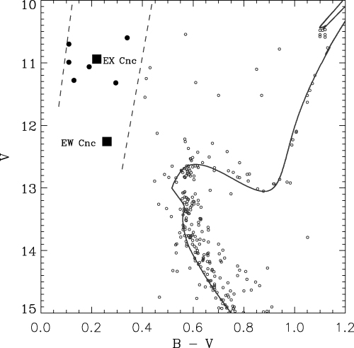
The colour–magnitude diagram of M67 based on standard B−V and V magnitudes. The solid line is an isochrone for an age of 4 Gyr. The locations of EW Cnc and EX Cnc have been marked with boxes and six other BSs in the instability strip (dashed lines) are marked with filled circles.
We characterize EW Cnc and EX Cnc using a grid of seismic models, but unlike Gilliland & Brown (1992) we also include the effects of rotation (in both equilibrium models and seismic oscillations). Rotation will affect the internal structure of the stars, induce mixing processes (Zahn 1992; Heger, Langer & Woosley 2000; Reese, Lignières & Rieutord 2006), and cause significant asymmetric splitting of multiplets even in these moderately rapid rotating stars (Saio 1981; Dziembowski & Goode 1992; Soufi, Goupil & Dziembowski 1998; Suárez, Goupil & Morel 2006).
2 BLUE STRAGGLER TARGETS
The locations of EW Cnc and EX Cnc in the colour–magnitude diagram of M67 are given in Fig. 1. We also analysed six other BS stars inside the instability strip and they are marked by filled circles. The B−V colours and V magnitudes are taken from Montgomery, Marschall & Janes (1993). Only stars observed during the present campaign are plotted. We have plotted an isochrone taken from the BaSTI data base (Pietrinferni et al. 2004) for an age of 4.0 Gyr with composition Z= 0.0198, Y= 0.2734, adopting a distance modulus of (m−M)V= 9.7. The instability strip is marked by dashed lines and is taken from Rodríguez & Breger (2001). It has been transformed from the Strömgren to the Johnson system using the calibration in Cox (2000). A finding chart showing the locations the BS targets is given in Fig. 2.
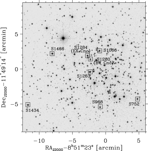
Finding chart for the BSs we have analysed with ID numbers from Sanders (1977). The image is from the STScI Digitized Sky Survey.
3 OBSERVATIONS
The data were collected in 2004 from January 6 to February 17 during a multisite observing campaign with nine 0.6- to 2.1-m class telescopes. The photometric reduction was done using the momf photometric package (Kjeldsen & Frandsen 1992, sections 5–6). The details of the observations and photometric data reduction were given in Paper I.
The choice of filters was made to optimize the S/N for the observations of the giant stars in M67 (see Paper II). All sites used the Johnson V filters except Kitt Peak, where a Johnson B filter was used. The bright BS star EX Cnc was saturated in about half of the B images. We have a total of 450 h of observation and about 15 000 data points for each star. The typical point-to-point scatter for EW Cnc and EX Cnc varies greatly from site to site, and lies in the range 1–8 mmag. By comparison, Gilliland & Brown (1992) used 37 h of observation to obtain 2458 CCD frames with 2-mmag point-to-point noise, which is similar to our best sites.
The complete light curve of EW Cnc is shown in the top panel in Fig. 3. The middle and bottom panels show the details of the light curves of EW Cnc and EX Cnc during 24 h. We have used different symbols for the five sites contributing to the light curve, as indicated in Fig. 3. The abbreviations for the five observatories are the same as in Paper I. The solid curves are the final fits to the complete data set (see Section 4.4).

The complete light curve of EW Cnc is shown in the top panel. The details of 24 h with nearly full coverage are shown in the two bottom panels for EW Cnc and EX Cnc where different symbols are used for each observing site. The continuous curves are the fits to the light curves.
4 TIME-SERIES ANALYSIS
4.1 Data point weights
As can be seen qualitatively in Fig. 3 and as described in detail in Paper I the quality of the photometry varied a lot from site to site, in many cases from night to night, and sometimes also during the night at a given site. To optimally extract the pulsation frequencies from the time-series we have assigned weights to each data point.
We calculated two kinds of weights: ‘scatter weights’ (Wscat), which are based on the scatter in the time-series and ‘outlier weights’ (Wout), which suppress extreme data points. The weights were calculated for each telescope and each star. The scatter weights were determined from the average point-to-point scatter in a large ensemble of reference stars, as described in detail in Section A1. To calculate the outlier weights, we used the deviation from zero of both the target star and the reference stars, as described in Section A2.
4.2 Combining observations in B and V
At Kitt Peak we used a Johnson B filter while all other sites used the Johnson V filter. The Kitt Peak data were collected simultaneously with several other sites (see fig. 2 in Paper I) but since the precision is far superior we decided to include it. The B filter data comprise 1459 data points (9 per cent) for EW Cnc and 598 points (4 per cent) for EX Cnc.
When combining the data we must correct for the dependence of the pulsation amplitude on the filter by scaling the B filter data. The scaling was found by measuring the amplitude ratios of the seven dominant frequencies in EW Cnc when using the B and V filters alone. The mean amplitude ratio was 0.74 ± 0.02,1 which is the scaling we applied. We also scaled the scatter weights found in Section A1 to ensure that the S/N is preserved. The mean phase shift is  , which is not significantly different from zero.
To make sure that our results are not affected by the inclusion of the scaled B data, we repeated the analysis described below when using only the V data. For both stars we found exactly the same frequencies except for two frequencies in EW Cnc and three frequencies in EX Cnc. The most significant of these frequencies has S/N = 5.2 while the others have S/N below 4.4. The slight differences we find in the frequencies and amplitudes are within the uncertainties found in Appendix B. We are therefore confident about combining the V data with the scaled B data.
4.3 The optimal amplitude spectrum
We calculated the amplitude spectrum both with the optimal spectral window and with the lowest noise level (see Kjeldsen et al. 2005). To do this we made the time-series analysis for two different approaches.
- Case A:
We computed the average light curve by binning all data collected within 8-min intervals. In the binning process we took into account the different quality of the data points by using weights WscatWout for n= 2 in equation (A3). We did not use weights when computing the amplitude spectrum a second time.
- Case B:
No binning, but each data point was given the weight WscatWout when calculating the amplitude spectrum.
It was case A that provided the optimal spectral window. The amplitude spectra of EW Cnc and EX Cnc for case A are shown in the top panels in Fig. 4. The residual spectrum after extracting the oscillation frequencies (see Section 4.4) is shown in each panel and the insets show the spectral windows, which have sidelobes at ±1 and ±2 c d−1 of ≃23 per cent.
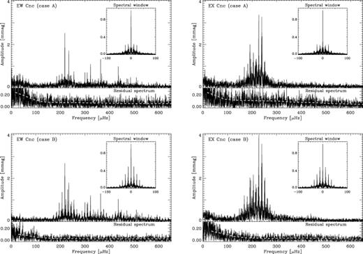
Amplitude spectra of EW Cnc (left-hand panels) and EX Cnc (right-hand panels) for the binned light curves (case A, top panels) and the noise-optimized light curves (case B, bottom panels). The residual spectrum is shown below each plot and the insets show the spectral windows. In the residual spectra the dashed grey lines mark the average noise level.
The lowest noise level was found in case B. We tried both n= 1 and 2 in equation (A3) but found that for n= 1 the noise level was 5–10 per cent lower, and in addition the ±1 c d−1 sidelobes were slightly lower. The fact that we found the lowest noise level for n= 1 indicates that 1/(WscatWout) is the best approximation to the true variance in the time-series. We note that this was also concluded by Handler (2003). The amplitude spectra for case B are shown in the bottom panels in Fig. 4.
While the noise level is significantly lower for case B, the spectral window has much lower sidelobes in case A. In Table 1 we compare the noise levels and aliases. The noise was calculated in a frequency band of 760 ± 60 μHz in the residual spectra.
For cases A and B we give the noise level in the amplitude spectrum at high frequencies (760 ± 60 μHz) and the height of the first alias peak in the spectral window. The results for our preferred cases are given in italics.
| Star | Case A | Case B | ||
| A760 (μmag) | Alias (per cent) | A760 (μmag) | Alias (per cent) | |
| EW Cnc | 55 | 23 | 37 | 48 |
| EX Cnc | 48 | 21 | 36 | 47 |
| Star | Case A | Case B | ||
| A760 (μmag) | Alias (per cent) | A760 (μmag) | Alias (per cent) | |
| EW Cnc | 55 | 23 | 37 | 48 |
| EX Cnc | 48 | 21 | 36 | 47 |
In Appendix B we have made simulations of the time-series to check whether case A or B gives the most robust results. The conclusion is that case A is preferred for EX Cnc due to the high number of frequencies found in a relatively narrow interval, while we use case B for EW Cnc. The results for these cases are given in italics in Table 1.
4.4 Fourier analysis of EW Cnc and EX Cnc
For each site the light curves were high-pass filtered to remove slow trends. In this way we suppressed variations with frequencies below 80 μ Hz, corresponding to periods longer than ≃3.5 h. The pulsation frequencies are found mainly in the intervals from 200 to 600 and 150 to 350 μHz for EW Cnc and EX Cnc, respectively. We used the period04 package by Lenz & Breger (2005) to fit the light curves in the frequency range 100–1000 μHz, as follows. The amplitude spectrum was calculated using the light curve from case B for EW Cnc and case A for EX Cnc (see Section 4.3). The highest peak was then selected and the frequency, amplitude and phase were fitted. This was done iteratively while in each step always improving the frequencies, amplitudes and phases of previously extracted frequencies.
We extracted 41 and 26 frequencies with S/N > 4 in the two stars, and the parameters are given in Tables 2 and 3. The uncertainties are based on simulations, as described in Appendix B. To determine the S/N of the extracted frequencies, we estimated the noise level in the amplitude spectrum around each frequency. This was done after cleaning the amplitude spectra so only peaks with S/N < 3 remained. The noise was calculated in bins with a width of 35 μHz and the noise estimate is the average of the three nearest bins for each frequency. The noise levels are marked by grey dashed lines in the residual spectra in Fig. 4.
Frequency, amplitude, phase and S/N of frequencies detected in EW Cnc for case B.
| ID | f (μHz) | a (mmag) | φ | S/N |
| f1 | 217.993(4) | 2.66(2) | 0.05(1) | 48.0 |
| f2 | 233.789(6) | 1.79(3) | 0.95(2) | 31.8 |
| f3 | 363.811(4) | 1.29(3) | 0.00(1) | 26.9 |
| f4 | 322.244(5) | 1.17(3) | 0.76(1) | 23.8 |
| f5 | 435.39(1) | 0.94(4) | 0.19(3) | 20.8 |
| f6 | 254.66(1) | 0.93(3) | 0.94(3) | 16.2 |
| f7 | 308.81(1) | 0.75(2) | 0.66(3) | 14.7 |
| f8 | 435.82(3) | 0.55(4) | 0.62(7) | 12.2 |
| f9 | 367.83(1) | 0.58(3) | 0.93(3) | 12.2 |
| f10 | 508.98(2) | 0.53(2) | 0.15(4) | 11.6 |
| f11 | 443.07(3) | 0.46(3) | 0.78(7) | 10.1 |
| f12 | 299.25(1) | 0.51(2) | 0.96(4) | 9.7 |
| f13 | 470.16(2) | 0.41(3) | 0.93(5) | 9.1 |
| f14 | 474.36(2) | 0.40(3) | 0.34(5) | 8.8 |
| f15 | 513.75(2) | 0.40(2) | 0.50(5) | 8.6 |
| f16 | 184.69(3) | 0.46(3) | 0.47(7) | 8.6 |
| f17 | 485.12(2) | 0.38(3) | 0.76(6) | 8.5 |
| f18 | 442.59(3) | 0.37(4) | 0.64(7) | 8.2 |
| f19 | 530.87(3) | 0.36(2) | 0.62(7) | 7.5 |
| f20 | 375.96(3) | 0.33(3) | 0.09(7) | 7.0 |
| f21 | 354.22(3) | 0.33(3) | 0.92(9) | 6.9 |
| f22 | 351.48(7) | 0.33(4) | 0.00(6) | 6.8 |
| f23 | 202.14(3) | 0.37(3) | 0.06(7) | 6.7 |
| f24 | 441.59(2) | 0.30(3) | 0.98(6) | 6.7 |
| f25 | 557.87(3) | 0.32(3) | 0.15(8) | 6.7 |
| f26 | 445.43(3) | 0.29(2) | 0.23(9) | 6.5 |
| f27 | 593.32(3) | 0.30(2) | 0.82(7) | 6.2 |
| f28 | 506.27(4) | 0.28(2) | 0.72(9) | 6.0 |
| f29 | 311.87(3) | 0.29(2) | 0.13(8) | 5.7 |
| f30 | 590.05(4) | 0.27(2) | 0.5(1) | 5.7 |
| f31 | 586.55(5) | 0.26(3) | 0.5(1) | 5.5 |
| f32 | 337.43(4) | 0.25(3) | 0.8(1) | 5.2 |
| f33 | 329.42(2) | 0.25(3) | 0.95(7) | 5.1 |
| f34 | 586.15(5) | 0.24(3) | 0.1(1) | 5.1 |
| f35 | 400.09(5) | 0.24(3) | 0.4(1) | 5.1 |
| f36 | 235.16(4) | 0.28(3) | 0.3(1) | 4.9 |
| f37 | 475.67(5) | 0.20(2) | 0.5(1) | 4.5 |
| f38 | 413.53(6) | 0.20(3) | 0.7(1) | 4.4 |
| f39 | 625.85(4) | 0.21(2) | 0.8(1) | 4.3 |
| f40 | 315.65(4) | 0.20(2) | 0.3(1) | 4.1 |
| f41 | 421.70(4) | 0.19(2) | 0.8(1) | 4.1 |
Frequency, amplitude, phase and S/N of frequencies detected in EX Cnc for case A.
| ID | f (μHz) | a (mmag) | φ | S/N |
| f1 | 226.910(4) | 3.87(6) | 0.94(1) | 36.2 |
| f2 | 238.883(5) | 3.74(6) | 0.60(1) | 35.0 |
| f3 | 240.297(8) | 2.31(7) | 0.97(2) | 21.7 |
| f4 | 191.464(9) | 2.08(7) | 0.45(2) | 18.3 |
| f5 | 226.45(1) | 1.79(8) | 0.28(3) | 16.7 |
| f6 | 205.49(1) | 1.68(8) | 0.14(3) | 15.2 |
| f7 | 228.66(2) | 1.33(8) | 0.57(4) | 12.4 |
| f8 | 215.33(1) | 1.34(8) | 0.41(4) | 12.3 |
| f9 | 196.96(1) | 1.18(7) | 0.71(4) | 10.5 |
| f10 | 190.92(1) | 1.16(8) | 0.46(3) | 10.2 |
| f11 | 217.43(2) | 1.05(8) | 0.28(5) | 9.6 |
| f12 | 211.82(2) | 1.04(7) | 0.77(4) | 9.5 |
| f13 | 196.15(2) | 0.83(7) | 0.03(4) | 7.4 |
| f14 | 193.93(2) | 0.79(7) | 0.11(6) | 7.0 |
| f15 | 219.95(2) | 0.75(7) | 0.89(6) | 6.9 |
| f16 | 236.34(2) | 0.60(5) | 0.04(7) | 5.6 |
| f17 | 203.19(3) | 0.62(7) | 0.64(8) | 5.6 |
| f18 | 223.01(4) | 0.59(7) | 0.19(9) | 5.5 |
| f19 | 258.86(3) | 0.58(6) | 0.27(8) | 5.5 |
| f20 | 199.45(3) | 0.59(7) | 0.76(7) | 5.3 |
| f21 | 234.39(4) | 0.55(6) | 0.5(1) | 5.2 |
| f22 | 229.14(5) | 0.55(5) | 0.5(1) | 5.2 |
| f23 | 250.65(2) | 0.48(8) | 0.85(6) | 4.5 |
| f24 | 256.86(3) | 0.47(6) | 0.55(9) | 4.4 |
| f25 | 182.09(3) | 0.50(6) | 0.69(8) | 4.4 |
| f26 | 148.54(3) | 0.49(6) | 0.20(7) | 4.3 |
In comparison Gilliland & Brown (1992) detected 10 frequencies in EW Cnc and six frequencies in EX Cnc. We recovered these frequencies except one of their weaker modes at 423.2 μHz in EW Cnc and at 186.5 μHz in EX Cnc. Zhang et al. (2005) detected four frequencies in EW Cnc and five frequencies in EX Cnc. They used data from a single observatory, and this explains why some of their frequencies are offset from ours by ±1 c d−1.
To check whether the frequencies we detected in the time-series analysis were reliable, we made the time-series analysis for both cases A and B. In both EW Cnc and EX Cnc we found that nearly all frequencies with S/N > 7 were detected2 in both cases, while this was not true for the weaker frequencies. Further, for the weaker frequencies that were detected in both cases there was sometimes an offset of 1 c d−1. In those cases, we chose the solution for case A, which has the better spectral window. As an additional check we used the 20 d in the time-series with the best coverage and were able to recover all frequencies with S/N > 6. We also used only the data set from La Silla (14 consecutive nights of observation) but found that for the weaker frequencies, the ±1 c d−1 alias was often identified as the most significant frequency, which is not surprising given the high sidelobes from the single-site time-series.
Several of the 41 frequencies found in EW Cnc are found to be linear combinations; examples are f5≃f13≃ 2 f1 and f18≃f5−f2≃f12−f28. We searched for combinations within twice the resolution of the data set which is Δf= 2/Tobs= 0.63 μHz. The condition is expressed as fi≃nfj+mfk for any integer value n, m∈[− 2;2] and i, j, k∈[1;41] and we found 13 combination frequencies. We compared this with 1000 sets of 41 randomly distributed numbers in the same interval as the observed frequencies, and we found 18 ± 6 combinations. Hence our detection of 13 linear combinations in EW Cnc is not surprising. However, none of the frequencies found in EX Cnc is found to be linear combinations. This is also the case for 1000 simulations of randomly distributed frequencies. The reason for the different results for the two stars is that the frequencies in EX Cnc are found in a much narrower frequency interval than for EW Cnc.
4.5 Interpretation of the EX Cnc spectrum
In both cases A and B, we see a clear pattern of nearly equally spaced peaks for EX Cnc (Fig. 4). In the top panel in Fig. 5 we show the amplitude spectrum of EX Cnc (case A) in more detail. To guide the eye we indicate a comb pattern with a separation of 1 c d−1(11.574 μHz) with dashed vertical lines. In the bottom panel the frequencies detected in case A (listed in Table 3) are marked by vertical lines.
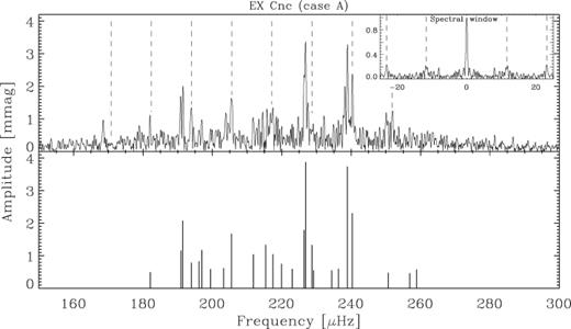
The top panel shows the amplitude spectrum of EX Cnc for case A. The inset shows the spectral window on the same horizontal scale as the main figure. The vertical dashed lines are separated by 1 c d−1 (11.574 μHz). In the bottom panel the detected frequencies are marked by vertical lines.
We note that each dominant peak in the comb pattern consists of several closely spaced peaks with remarkable similarity to what is seen for stochastically excited and damped oscillations, also called solar-like oscillations, which are driven by convection (Anderson, Duvall & Jefferies 1990). We investigated whether the observed regular pattern and the closely spaced lower amplitude peaks around each dominant peak could be explained by
stochastically excited and damped oscillations of equally spaced modes;
the spectral window (alias peaks);
closely spaced modes.
In δ Scuti stars, the oscillations are caused by the κ mechanism (opacity driven) and are believed to be coherent, which will produce a single isolated peak for each oscillation mode in the amplitude spectrum. Although damped oscillations driven by convection might be present in some δ Scuti stars (Samadi, Goupil & Houdek 2002), the expected frequencies and amplitudes are very different from what we see in Fig. 5, which is consistent with opacity-driven oscillations. The calculations by Samadi et al. (2002) show frequencies in the range 400–1200 μHz and amplitudes of roughly 100 ppm for their selected models. These values are consistent with what we found specifically for this star using the parameters in Table 5, a mass of 2 M⊙, and the usual scaling relations to predict the characteristics of solar-like oscillations (Brown et al. 1991; Kjeldsen & Bedding 1995). We find the central frequency (maximum amplitude) to be νmax≃ 630 μHz, amplitudes δL/L≃ 40 ppm and mean frequency separation Δν0≃ 40 μHz). These properties of solar-like oscillations are clearly inconsistent with the observed amplitude spectrum.
Simulations showed that the regular pattern was unlikely to be the result of only two or three modes. To reproduce the observed amplitude spectrum required at least four to five modes, equally spaced by roughly 1 c d−1. The low alias sidelobes, especially in case A, imply that the pattern is intrinsic to the star. Many of the lower amplitude peaks around each dominant peak seem to be separated by exactly 1 or 2 c d−1 from a neighbouring peak. However, the strengths of these lower amplitude peaks are in many cases higher than expected from the strengths of the sidelobes in the spectral window.
Closely spaced peaks are not uncommon in δ Scuti stars (Breger & Bischof 2002). Breger & Pamyatnykh (2006) noted that 18 pairs (Δf < 1μHz) exist in the δ Scuti star FG Virginis (Breger et al. 2005). They found evidence for the frequency doublets being real. As seen in Fig. 5, we also detect several close pairs.
Fundamental parameters of EW Cnc and EX Cnc.
| EW Cnc | EX Cnc | |||
| Teff (K) | log g | Teff (K) | log g | |
| Mathys (1991) | 8090 | 4.33 | 7750 | 3.79 |
| Gilliland & Brown (1992) | 7960 | 4.20 | 7900 | 3.88 |
| Landsman et al. (1998) | 8090 | 4.12 | 7610 | 3.78 |
| uvby (this study) | 7800 | 7840 | ||
| Geneva (this study) | 8080 | 4.59 | ||
In summary, damped oscillations driven by convection seems to be a very unlikely cause for the characteristic pattern we see in Fig. 5. We believe the pattern is most likely due to a nearly regular series of at least five modes (excited by the κ mechanism) which, due to a general spacing very close to 1 c d−1, shows a large number of small peaks around each dominant peak caused by the spectral window. This is further enhanced by the presence of lower amplitude modes close to the dominant modes (see bottom panel in Fig. 5). Our interpretation is supported by Gilliland & Brown (1992) who found frequency separations of ∼5 and ∼10 μHz in this star, and suggested that the latter might be due to rotational splitting.
4.6 A search for pulsations in six other BS stars
In addition to EW Cnc and EX Cnc, we observed six other BS stars in the instability strip as shown in Fig. 1. To search for pulsations in the stars we calculated the amplitude spectra in the range 0–1000 μHz, using weights as for case B (Section 4.3). In Table 4 we summarize the properties of the BS stars observed during the campaign. For completeness, EW Cnc (S1280) and EX Cnc (S1284) are included in the table. We give the ID numbers from Sanders (1977) and Montgomery et al. (1993), and the V magnitude, and B−V colour from the latter. The total number of data points N and σint (equation A1) for the La Silla and LOAO (Mt Lemmon Optical Astronomy Observatory) sites indicate the quality of the data. We note that La Silla had very good weather conditions during the campaign, while LOAO had worse conditions (for more details see Paper I). The mean level in the amplitude spectrum in the range where oscillations are expected is denoted A350 (200–500 μHz), while that at slightly higher frequencies A760 (700–820 μHz) is a measure of the white noise. In the last column, the membership probability from Sanders (1977) is given. We note that more recent radial velocity studies by Girard et al. (1989) and Zhao et al. (1993) are in general agreement with this.
Properties of the light curves and amplitude spectra of the observed BS stars in M67. Star ID from Sanders (1977) and ID, V, and B−V from Montgomery et al. (1993) are given. N is the number of data points. The point-to-point scatter at the LaS and LOAO sites and the noise level in the amplitude spectrum in the range 350 ± 150 μHz and 760 ± 60 μHz are listed. The last column contains membership probabilities from Sanders (1977).
| Name | Sanders | MMJ | V | B−V | N | σLaS (mmag) | σLOAO (mmag) | A350 (μmag) | A760 (μmag) | PMember (per cent) |
| S1466 | 6511 | 10.60 | 0.34 | 13 316 | 1.7 | 3.3 | 66 | 41 | 0 | |
| S1434 | 6510 | 10.70 | 0.11 | 3312 | – | 3.3 | 372 | 160 | 91 | |
| EX Cnc | S1284 | 6504 | 10.94 | 0.22 | 14 660 | 1.9 | 2.9 | 240 | 65 | 95 |
| S1066 | 6490 | 10.99 | 0.11 | 16 954 | 1.7 | 2.6 | 46 | 35 | 90 | |
| S1263 | 6501 | 11.06 | 0.19 | 17 408 | 4.6 | 2.7 | 89 | 69 | 89 | |
| S968 | 6479 | 11.28 | 0.13 | 9851 | 1.5 | 2.9 | 55 | 37 | 95 | |
| S752 | 6476 | 11.32 | 0.29 | 3316 | – | 2.8 | 194 | 120 | 95 | |
| EW Cnc | S1280 | 5940 | 12.26 | 0.26 | 15 524 | 1.9 | 3.3 | 188 | 46 | 93 |
Two of the BS stars (S1434 and S752) were only observed by a few sites. Hence, for these stars the noise level in the amplitude spectrum is about a factor of 4–6 higher than for the other stars. We find no significant peaks in the range 0–1000 μHz above S/N of 43 in any of the BS stars except EW Cnc and EX Cnc.
Our results are in agreement with Sandquist & Shetrone (2003) who looked for photometric variability in several BS stars in M67. Except for EW Cnc and EX Cnc they found no δ Scuti pulsations in their sample, which included S752, S968, S1066 and S1263. The latter was also observed by Gilliland & Brown (1992) who placed an upper limit of variation at 0.2 mmag (corresponding to ∼5 mmag scatter in the time-series) for frequencies above 130 μHz, in agreement with this study and Sandquist & Shetrone (2003). We note that Stassun et al. (2002) reported unusually high scatter of up to 30 mmag in this star from a photometric BVI time-series study. The relatively high noise level for S1263 compared to the other BSs in our data (see σLaS in Table 4) is due to the star being blended (see Fig. 2).
5 THEORETICAL MODELS OF EW AND EX Cnc
To model EW Cnc and EX Cnc we used the stellar evolution code cesam (Morel 1997). The effects of rotation are taken into account in the equilibrium equations as a first-order perturbation to the local gravity, while assuming rotation as a rigid body. The ceff equation of state was used (Christensen-Dalsgaard & Daeppen 1992) and opal opacities were adopted (Iglesias & Rogers 1996). A more detailed description of the input physics for the cesam code was given by Casas et al. (2006).
We used the oscillation code filou (Tran Minh & Leon 1995; Suárez 2002) to calculate the oscillation frequencies from the evolution models. We assume rigid-body rotation and the effects up to second order in the centrifugal and Coriolis forces were included. We note that Reese et al. (2006) found that this perturbation approach may be invalid even at moderate rotational velocities. Effects of near degeneracy are expected to be significant (Soufi et al. 1998) as was described in detail by Suárez et al. (2006).
5.1 Fundamental atmospheric parameters
The fundamental atmospheric parameters of EW Cnc and EX Cnc were estimated by Mathys (1991) and Gilliland & Brown (1992) based on Strömgren photometry by Nissen, Twarog & Crawford (1987) but applying different calibrations (Philip & Relyea 1979; Moon & Dworetsky 1985). We used the more recent calibration by Napiwotzki, Schoenberner & Wenske (1993), while assuming the mean cluster reddening from Nissen et al. (1987). For EW Cnc we used Geneva photometry from Rufener (1976) and applied the calibration by Kunzli et al. (1997). Landsman et al. (1998) constrained Teff of both stars based on UV measurements. We summarize the results in Table 5. Typical uncertainties on Teff and log g are 150 K and 0.2 dex and there is good agreement between the different calibrations.
An important limitation of our modelling is the uncertainty on the composition of the stars. The composition will depend on the formation scenario of these BS stars, which we certainly cannot begin to constrain with the current data set. Gilliland & Brown (1992) discussed different formation scenarios for the same stars from either a direct collision or gradual coalescence. They made the important point that it would be difficult to detect the effects of a 5 per cent increase of helium, for example, as a result of mixing two evolved main-sequence stars. For simplicity we assume that the metallicity of EW Cnc and EX Cnc is the same as for the cluster. Montgomery et al. (1993) found [Fe/H]=−0.05 but they did not estimate the uncertainty; a conservative estimate is ±0.10 dex.
5.2 The model grid
We have calculated a grid of stellar models consistent with the fundamental parameters of EW Cnc and EX Cnc. A few evolution tracks are shown in Fig. 6 in the log g versus Teff diagram, where the solid and dashed lines correspond to rotational velocities of 65 and 120 km s−1. The photometric error boxes are shown as grey squares. The centre of each box is the Teff and log g from Landsman et al. (1998) and the half-widths are equal to the estimated uncertainties of 150 K and 0.2 dex. We have computed pulsation frequencies for the models inside the photometric error boxes. The mass ranges are 1.7 –2.0 M⊙ for EW Cnc and 1.8 –2.3 M⊙ for EX Cnc in steps of 0.1 M⊙. Further details of the grid of pulsation models are given in Table 6.
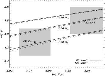
The log g–Teff diagram showing selected evolution tracks from our model grid. The 1σ photometric error boxes of EW Cnc and EX Cnc are indicated as grey squares.
Parameters of theoretical pulsation models for EW Cnc and EX Cnc, which are inside the photometric error boxes shown in Fig. 6. For each mass the range of effective temperatures is given. For each star we computed models with two different rotational velocities given in the last column.
| Star | M/M⊙ | Teff (K) | vrot (km s−1) |
| EW Cnc | 1.7 | 7930–8110 | 90, 150 |
| 1.8 | 7930–8210 | – | |
| 1.9 | 7930–8210 | – | |
| 2.0 | 7940–8200 | – | |
| EX Cnc | 1.8 | 7450–7620 | 65, 120 |
| 1.9 | 7450–7740 | – | |
| 2.0 | 7480–7740 | – | |
| 2.1 | 7470–7710 | – | |
| 2.2 | 7480–7730 | – | |
| 2.3 | 7630–7740 | – |
Analyses of stellar spectra (Peterson, Carney & Latham 1984; Manteiga, Martinez Roger & Pickles 1989; Pritchet & Glaspey 1991) reveal moderate projected rotational velocities for EW Cnc and EX Cnc, and we have used average values of v sin i= 90 and 65 km s−1, respectively. However, the inclination angle is unknown, and therefore we calculated models and corresponding oscillation frequencies for the minimum and a moderate value of vrot for each star. The values in the last column in Table 6 correspond to inclination angles of i= 90° and 45°.
5.3 Comparison of observed and theoretical frequencies
In Fig. 7 we show the number of modes as a function of frequency, in bins of 50 μHz. The black histograms are for the observed frequencies for EW Cnc (left-hand panels) and EX Cnc (right-hand panels), which are listed in Tables 2 and 3. The solid histograms are for frequencies from pulsation models and the colours indicate how high angular degree, l, we have included.4 The top and bottom panels are for models with high and low mass. The low-mass models both have a mass 1.8 M⊙, while the high-mass models correspond to the evolution tracks that graze the photometric error boxes, that is, 2.0 and 2.3 M⊙ for EW Cnc and EX Cnc, respectively. We used the Teff adopted for the centres of the photometric error boxes in Fig. 6.
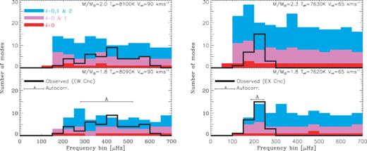
Histograms showing the number of frequencies in EW Cnc (left-hand panel) and EX Cnc (right-hand panel) in frequency bins of 50 μHz. The filled histograms are for pulsation models and the colour describes how high angular degree is included. The thick black lines are for the observations. The top and bottom panels are for pulsation models with high and low mass with the adopted Teff. The models in the bottom panels both have mass 1.8 M⊙, slightly different vrot and quite different Teff. The horizontal bar marked ‘A’ marks the region used for the autocorrelation in Section 5.3.
By inspecting the histograms for the models in Fig. 7 one can see that the number of modes increase when increasing the mass or decreasing Teff. Histograms for models with different rotational velocities are nearly identical since the frequency shifts are relatively small (≃few μHz) for these moderate velocities. The histograms of all pulsation models within the photometric error boxes are in agreement with the observations, but only when including modes with degrees l= 0, 1 and 2. However, if the masses are lower than 1.7 and 1.8 M⊙ for EW Cnc and EX Cnc, respectively, it will require lower temperatures, which are outside the photometric error boxes. In other words, if a more accurate Teff becomes available we can put a lower limit on the mass.
In EW Cnc the detected frequencies are evenly distributed over a wide interval, while in EX Cnc they are concentrated in a narrow band. The horizontal bars labelled ‘A’ in Fig. 7 indicate where most observed frequencies are found. In these frequency intervals we estimate that we have detected 40–60 per cent of the modes in EW Cnc and 70–100 per cent in EX Cnc. These results rely on the assumptions that the considered ranges in mass and Teff are realistic and that only l≤ 2 modes have detectable amplitudes.
To further investigate the distribution of peaks and search for recurring patterns we computed autocorrelations for the frequencies from the observations and the pulsation models. This method can in principle be used to extract important quantities for asteroseismic modelling like the large and small separation and rotational splitting. This would enable us to constrain the mass and temperature of the stars. Since we have no information about the relative amplitudes of the theoretical frequencies, each frequency is represented by a Gaussian of unit height and with a full width at half-maximum equal to twice the formal frequency resolution of the data set. To be able to compare the autocorrelations of the observed and theoretical frequencies, we follow the same procedure for the observations, that is, only using the frequencies and not the observed amplitudes. We use the frequencies from the regions where the majority of the frequencies are observed. These regions are marked by horizontal bars labelled ‘A’ in Fig. 7. We tried different widths of these bands, but the conclusion summarized here is the same.
In Fig. 8 we show autocorrelations for theoretical and observed frequencies for EW Cnc (left-hand panels) EX Cnc (right-hand panels). The models have the same masses and temperatures as shown in the histograms in Fig. 7. In the top panel only radial modes are included. The results for EX Cnc shows the large separation at ≃23 μHz for the model with high mass, while for the less massive model there is a low peak at twice the large separation (see top right-hand panel in Fig. 8). In the middle panel we included all model frequencies with l= 0, 1 and 2; the higher number of modes makes the interpretation of the autocorrelation much more difficult. In the bottom panels we show the autocorrelations of the observed frequencies. There is an intriguing similarity between the autocorrelation of the observed frequencies in EX Cnc and the model with high mass (the middle and bottom right-hand panels in Fig. 8). However, we are extremely cautious not to overinterpret the only marginally significant autocorrelation peaks at 2, 6, 12 and 24 μHz.
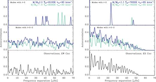
Comparison of the autocorrelations of frequencies from pulsation models and the observed frequencies in EW Cnc (left-hand panels) and EX Cnc (right-hand panels). In the top panels we included only radial modes while in the middle panel we included modes with l= 0, 1 and 2. We show results for the same models as in Fig. 7. The bottom panels are the autocorrelations of the observed frequencies.
Although there appears to be qualitative agreement between the observations and the theoretical models, we cannot at this stage use the method to determine which combination of mass, evolutionary stage or rotational velocity best describes the observations. To make progress and make a detailed comparison of the observed frequencies with theoretical models would require that we have identified at least some of the dominant modes. This can be achieved from the study of line-profile variations or from comparison of phase shifts of the frequencies in different photometric filters (Daszyńska-Daszkiewicz, Dziembowski & Pamyatnykh 2003). We cannot apply the latter method since most of our observations were done in the V band with only a few nights of data in B.
6 CONCLUSION
We have analysed a new photometric data set of eight BS stars in M67. Only in the two known variable stars EW Cnc and EX Cnc do we find δ Scuti pulsations. We detect 41 frequencies in EW Cnc and 26 frequencies in EX Cnc. Compared to the previous multisite campaign by Gilliland & Brown (1992) we have detected four times as many frequencies in these two stars, and the number of frequencies is comparable to the best studied field δ Scuti stars.
The frequencies with the highest amplitudes in EX Cnc are separated by roughly 1 c d−1 (see Fig. 5) and our extensive multisite data are therefore essential to study the pulsations in this star. We have made simulations of the light curves which show that the frequencies are recovered in all cases (see Appendix B). We repeated the Fourier analyses on subsets of the data to confirm that the same frequencies were extracted. Thus, we claim that the observed pattern cannot be due to the spectral window, but represents a real property of the distribution of frequencies in EX Cnc. Additional support for this claim is the fact that a similar pattern is not seen in EW Cnc.
We computed a grid of theoretical pulsation models that take the effects of rotation into account, which were not included in earlier models (Gilliland & Brown 1992). We find general agreement between the observed and computed frequencies when comparing their distribution in histograms. We can claim to have detected non-radial modes and in the range where most of the frequencies are observed, and at least 40 and 70 per cent of all low-degree (l≤ 2) modes are excited in EW Cnc and EX Cnc, respectively. This is perhaps the most important result of the current study, since in the past decade of observational work on δ Scuti stars only a tiny fraction of the frequencies expected from theoretical models were in fact detected. A reasonable explanation is that high S/N and good frequency resolution is needed to be able detect the weakest modes as was suggested by Breger et al. (2005) and Bruntt et al. (2007).
The autocorrelation of the observed frequencies does not show any significant peaks in any of the stars. However, autocorrelations of the frequencies from theoretical pulsation models show that if indeed modes with degree l= 0, 1 and 2 are observed, we cannot expect to unambiguously detect the large separation from such an analysis. This result was obtained while assuming that all amplitudes are equal, since no amplitude information is available for the theoretical models.
To improve on the interpretation of the rich frequency spectra of EW Cnc and EX Cnc, and other well-observed δ Scuti stars in general, we see two possibilities.
On the theoretical side, it would be very helpful to have estimates of the amplitudes of the modes. If relative amplitudes could be reliably estimated from theory the autocorrelation might be a useful method for measuring the separation between radial modes and hence constrain the density of δ Scuti stars.
On the observational side we need to be able to identify the degrees of at least the main modes. This can in principle be done by comparison of phases and amplitude ratios for different narrow-band filters as has been attempted for other δ Scuti stars (Moya, Garrido & Dupret 2004; Daszyńska-Daszkiewicz et al. 2005).
We have too few observations in the B filter to follow the latter suggestion, and multifilter (e.g. Strömgren by) observations should be considered for similar campaigns in the future. The points mentioned here also apply when planning ground-based support for the CoRoT (Michel et al. 2006) and Kepler (Basri, Borucki & Koch 2005) satellite missions. These missions will provide photometric time-series with long temporal coverage of several δ Scuti stars, but only in a single filter.
On request we would gladly provide the light curves presented here.
Koen et al. (2001) observed two single-mode δ Scuti stars (HD 199434 and HD 21190) in the B and V filters and found amplitude ratios of 0.70 ± 0.01 and 0.70 ± 0.03, respectively. We note that the empirical scaling is close to the ratio of the central wavelengths, that is, λB/λV= 434 nm/ 545 nm ≃0.80.
The S/N was measured for case B.
Defined as 4 A350 where A350 is from Table 4.
In the integrated light from the stars we expect to observe only low-degree modes. Modes with l≥ 3 will have very low observed amplitudes due to geometrical cancellation effects when averaging over the stellar disc. We note that for each mode we include all 2l+ 1 possible values of m.
The neighbouring data points were required to be within a certain time-limit, set arbitrarily to 10 times the median time-step between frames (for a given telescope). If there was only one neighbouring data point, we used only this to compute the deviation δr. If there were no neighbouring data points within the time-limit (rarely the case), we assigned a weight that was the mean of the weights of data points just before and after the point in question.
Note that the stellar oscillations were subtracted before calculating outlier weights.
Recall that Wout is the mean of Wr for all reference stars r.
This work was partly supported by the Research Foundation Flanders (FWO). HB was supported by the Danish Research Agency (Forskningsrådet for Natur og Univers) and the Instrument centre for Danish Astrophysics (IDA). HB and DS were supported by the Australian Research Council. This paper uses observations made from the South African Astronomical Observatory, Siding Spring Observatory in Australia, Mount Laguna Observatory operated by the San Diego State University, the Danish 1.54-m telescope at ESO, La Silla, Chile, Sobaeksan Optical Astronomy Observatory in Korea, and Mt Lemmon Optical Astronomy Observatory in Arizona, USA, which was operated remotely by Korea Astronomy and Space Science Institute.
REFERENCES
Appendices
APPENDIX A: DATA POINT WEIGHTS
This appendix contains a detailed description of how we calculated weights using an ensemble of reference stars (cf. Section 4.1). The reference stars were chosen from the most isolated stars, that is, stars with a maximum of 10 per cent flux from neighbouring stars within their photometric apertures. Furthermore, we required that their point-to-point scatter was close to the theoretical limit as determined by photon noise. The observations from LOAO had the greatest field of view with a total of 358 stars. For this site we used M= 65 reference stars. For the site with the smallest CCD we used only 40 reference stars. In Fig. A1 we show the average point-to-point scatter (σint, see equation A1 below) for the stars at the LOAO site plotted versus V magnitude. The solid grey line marks the fiducial σint, fiduc that represents the typical scatter for the best stars at a given magnitude. The reference stars are marked with filled circles, and the inset shows the location of the stars in the colour–magnitude diagram.
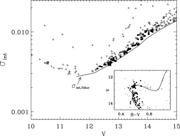
Internal scatter in the light curves of bright stars observed at the LOAO site. The grey line marks the fiducial σint, fiduc. The filled circles mark the reference stars used for measuring weights. The inset shows the location of the stars in the colour–magnitude diagram of M67.
A1 Determination of scatter weights: Wscat

 , and calculated the scatter weight as
In Fig. A2 we show the light curve versus data point number for one reference star in the top panel. These data are from the Wide Field Imager (WFI) at Siding Spring, Australia. In the bottom panel we plot the derived scatter weights normalized so that the highest weight equals 1. The dashed horizontal line marks the limit for data points with scatter weights Wscat < 25 per cent. These points are plotted with grey symbols in the top panel as well.
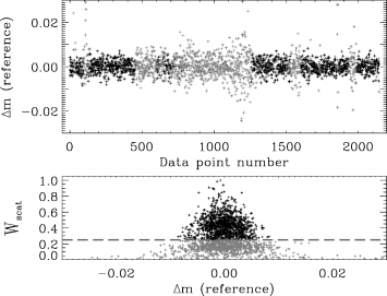
The top panel shows the light curve of a reference star from WFI. The grey points have scatter weights Wscat < 25 per cent. The bottom panel shows the scatter weight found using all the reference stars. The dashed horizontal line marks the 25 per cent level.
A2 Determination of outlier weights: Wout
 using all M reference stars. In equation (A4), Δmt is the deviation from zero for the target star and σt is an estimated scatter. Likewise, Δmr and σr are the corresponding values for the rth reference star. The values of at and ar determine how much a data point must deviate before the outlier weight becomes significantly smaller than 1. For the target star we used at= 3 and for the reference stars we used ar= 2. Thus, data points that lie within 3σ for the target star, and within 2σ for the majority of the reference stars will not get low outlier weights. The exponent b describes how steeply Wr decreases from one to zero. We used the value b= 4. To estimate the scatter σ in equation (A4) for the target and reference stars, we use the scatter weights Wscat from Section A1. We approximate σ=σintη, where σint is computed from equation (A1) and η=〈Wscat〉/Wscat, where 〈Wscat〉 is the average scatter weight over the entire series. Thus, η is a measure of the relative change in scatter from frame to frame.
To illustrate the process we have plotted the light curve of a reference star versus the target star EW Cnc6 in Fig. A3. The grey ellipse has half-major and half-semimajor axes corresponding to 3σint for each star. Intuitively, there are too many points outside this ‘3σ ellipse’. If the noise were Gaussian, the fraction of points that would fall outside the 3σ limit would be only  . This corresponds to only 24 out of 2150 data points from WFI, while about 100 are found in the data. The large black dots in Fig. A3 have outlier weights Wr < 0.5 and small points have 1 ≥Wr≥ 0.5.
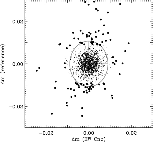
The light curve of a reference star is plotted versus a target star (EW Cnc) for data from WFI. The large black dots have outlier weights Wr < 0.5. We plot the ‘3σ ellipse’ in grey colour (see text for details).
In Fig. A4 we show the light curves of EW Cnc and the same reference star as in Fig. A3. For the reference star (top panel) the filled circles mark data points with low outlier weights, that is, Wr < 0.5. The data points of the target EW Cnc are shown in the bottom panel in Fig. A4. We have marked the points with final outlier weights Wout < 0.5 with filled squares.7 It is interesting to note that several data points are not obvious outliers. In fact some of the marked outliers have, for example, Δm < 2σ, where σ is the local rms scatter. The reason for these points having Wout < 0.5 is that they were outliers in most of the reference stars.

In the top panel the light curve of a reference star is shown, where filled circles have reference star outlier weights Wr < 0.5. The light curve of the target star (EW Cnc) is shown in the bottom panel, where filled boxes have final outlier weights Wout < 0.5 (see text for details).
APPENDIX B: LIGHT-CURVE SIMULATIONS
Simulating the light curves has two goals.
To measure our ability to extract the inserted modes for cases A and B and decide which one is optimal.
To measure the uncertainty on the frequency, amplitude and phase.
The simulated light curves were constructed to have the same noise characteristics as for the observations. To measure the properties of the noise in the observations, we first subtracted the detected frequencies before computing the amplitude spectrum. We used two components to describe the white noise and the drift noise.
The white noise was measured as the mean level in the observed amplitude spectrum in the frequency range 1000–1500 μHz.
The drift noise leads to an increase in the noise level towards low frequencies. This ‘1/f’ noise was measured by fitting a fiducial spline function to the observed increase in noise in the amplitude spectrum.
Since each site had a different white noise component and a different shape of the 1/f noise we constructed the light curve site by site before adding the data as we did for the actual observations.
In practice, we created an evenly sampled light curve covering the time-span of the observed time-series, but with an oversampled grid in time by a factor of 5. Each light curve consists of random numbers with different seed number. The mean is zero and the numbers have a point-to-point scatter corresponding to the noise level found in step (1). First, we take the Fourier transform of the light curve to the frequency domain, and multiply the result by the fiducial spline fit found in step (2). We then take the Fourier transform to return to the time-domain, and pick the synthetic data points closest in time to the observed data points. Finally, we add the frequencies detected in the star. For each star 50 simulations were realized.
We made a Fourier analysis of each simulation as we did for the observed data (see Section 4.3). In Fig. B1 we show how often each inserted frequency was recovered in the simulations versus S/N. The top and bottom panels are for EW Cnc and EX Cnc, respectively. In each panel open and filled symbols correspond to cases A and B (Section 4.3). For EW Cnc it is seen that in both cases A and B all frequencies with S/N > 5 are recovered. We prefer case B for EW Cnc since it has a significantly lower residual noise level (see Table 1). For EX Cnc we choose case A because it shows a much better recovery rate than case B.
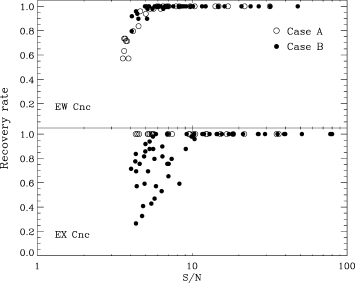
Recovery rates of frequencies inserted in the simulations of EW Cnc (top panel) and EX Cnc. The results for cases A and B are shown with open and filled symbols, respectively.
The uncertainties on frequency, amplitude and phase given in Tables 2 and 3 are computed from the rms scatter in the simulations. We plot the uncertainties versus the amplitudes for EW Cnc (case B) and EX Cnc (case A) in Fig. B2. The dashed lines are theoretical lower estimates of the uncertainties using the expressions from Montgomery & O'Donoghue (1999) which are valid for uncorrelated noise, that is, for data with only a white noise component. For real data one must multiply the uncertainty by the square root of the estimated correlation length (Montgomery & O'Donoghue 1999). We found this by calculating the autocorrelation of the residual amplitude spectrum after the mean value has been subtracted. The intersection of the autocorrelation function with zero is a measure of the correlation length, D. For both EW Cnc and EX Cnc we find D= 3.2 ± 0.1 or  . The resulting estimates of the uncertainties are marked by the solid lines in Fig. B2.
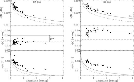
Uncertainties of frequency, amplitude and phase based on simulations of EW Cnc (left-hand panels) and EX Cnc (right-hand panels). The dashed lines are theoretical lower estimates from Montgomery & O'Donoghue (1999), while the solid lines result from multiplying by the correlation length  .
.
In general we find an acceptable agreement with the estimated uncertainties from Montgomery & O'Donoghue (1999). For most parameters the estimated uncertainties are too low, especially so for the frequencies and phases in EX Cnc. This is likely because the frequencies lie closer in EX Cnc compared to EW Cnc. The uncertainties on the amplitudes in EW Cnc are close to the estimate for uncorrelated noise.
