Analysis of the effect of a mean velocity field on a mean field dynamo

Abstract

1 INTRODUCTION

Magnetohydrodynamical (MHD) turbulence seems to be a major physical process to generate and maintain the magnetic fields observed in most of the structures of the Universe (Zel'dovich et al. 1983; Brandenburg & Subramanian 2005a). When addressing the problem of the generation of large-scale magnetic fields by small-scale turbulent flows, a model known as mean field dynamo (MFD) is usually considered (Moffatt 1978). Despite its simplicity and lack of broad applicability, it proved to be a very useful tool in studying qualitatively conceptual issues of large-scale magnetic field generation. The mechanism is based on decomposing the fields into large-scale, or mean fields, ⁠, and small-scale, turbulent ones u, b, a. These small-scale fields have very small coherence length, but their intensities can be higher than that of the mean fields. In this mechanism, the evolution equation for is written as ⁠, where is the Ohmic resistivity and the turbulent electromotive force (TEMF).1 The term is usually disregarded in the studies of MFD as the focus of most of them is to understand the generation of large-scale quantities due to small-scale effects. If homogeneous and isotropic turbulence is considered, the TEMF can be written as ⁠, with and being a correlation time (Moffatt 1972; Rudiger 1974; Pouquet, Frisch & Leorat 1976; Zel'dovich et al. 1983). The dependencies on and b are due to the back-reaction of those induced fields on the dynamo (Moffatt 1978; Brandenburg & Subramanian 2005a). In the kinematically driven dynamo considered here, the features of the generated fields crucially depend on the helicity of the flows: helical flows are at the base of the mechanisms to generate large-scale fields, while non-helical flows would only produce small-scale fields. This separation, however, is somewhat artificial, as small-scale fields are also produced by helical turbulence (Brandenburg & Subramanian 2005a).

In this paper, we want to address an issue not (or very seldom) considered in the literature up to now, namely, the induction of large-scale flows ⁠, also named shear flows, by the small-scale turbulent fields, and how these induced flows back-react on the turbulent electromotive force of a MFD. On one side, we mean that the expression would be valid only during the time interval in which ⁠, and on the other, even if this condition is satisfied, could be affected by the generation of and consequently its functional form should be modified to incorporate this effect. The generation of magnetic fields due to the action of these large-scale velocity flows instead of by was recently addressed analytically by several authors (Rogachevskii & Kleeorin 2003, 2004; Rädler & Stepanov 2006), and was also studied numerically by Brandenburg (2001) and semi-analytically by Blackman & Brandenburg (2002). However, none of those works specifically addressed the issue we want to analyse here.

We work in the framework of the two-scale approximation that consists of assuming that mean fields peak at a scale k⁻¹_L while turbulent ones do so at k⁻¹_S≪k⁻¹_L, and also consider homogenous and isotropic turbulence. Although this kind of turbulence is of dubious validity when dealing with large-scale fields, it serves well for initial, qualitative studies of the sought effects. Another assumption we will make is that is force-free, i.e. of maximal current helicity. Although fields with this feature can be observed in certain astrophysical environments, they are not a generality, and also they are not seen in some numerical simulations. The main reason to use them here is to simplify the (heavy) mathematics, while maintaining a physically meaningful scenario.

In order to find when Lorentz force acts on the plasma, we must solve a differential equation that contains terms with one-point triple correlations, i.e. averages of products of three stochastic fields evaluated at the same point. This means that instead of dealing with only one equation to solve for ⁠, we have to solve a hierarchy of them. In order to break this hierarchy and thus simplify the mathematical treatment of the problem, we must choose a closure prescription, which consists of writing the high-order correlations as functions of the lower order ones, but maintaining the physical features of the problem under study. In MHD, the intensity of the non-linearities is measured by the magnetic Reynolds number, which is defined in the induction equation for the magnetic field, ∂B/∂t=∇(U×B) +η∇²B, as R_m∼ (UB/l) /(ηB/l²) =Ul/η, where U is a characteristic velocity of the plasma, l is a characteristic length and η is the ohmic resistivity. Thus, for R_m≪ 1 the non-linear terms can be neglected in front of the resistive ones, and therefore the equations become linear, while for R_m≫ 1 the resistive terms should be dropped off in front of the non-linear ones. The intermediate regime is more difficult to analyse. In this paper, we will consider R_m≫ 1, i.e. the non-linearities must be maintained and, consequently, a closure scheme must be selected to deal with them. We choose to work with the so-called minimal τ approximation (Blackman & Field 2002; Brandenburg & Subramanian 2005a), whereby the triple moments in the equation for will be considered as proportional to quadratic moments, and written in the form ⁠, with the proportionality factor ζ∼τ⁻¹_rel, where τ_rel is a relaxation time that can in principle be scale, and/or R_m, dependent. The validity of this closure was checked numerically (Brandenburg & Subramanian 2005b) for low Reynolds numbers, and was also verified for the case of passive scalar diffusion. We will assume that it is also valid for all the triple correlations that may appear throughout this work. We consider boundary conditions such that all total divergencies vanish. These conditions may be a bit unrealistic for astrophysical systems, but they have two advantages: magnetic helicity becomes a gauge-invariant quantity (Berger & Field 1984) and the obtained results can be compared with numerical simulation, as to perform them it is customary to use those conditions. We consider fully helical, prescribed, u fields.

Our starting points are the evolution equations for and for the magnetic helicities H^M_L,S, as the evolution of these quantities is tightly interlinked (Blackman & Field 2002; Brandenburg & Subramanian 2005a) in the absence of shear flows. When including new terms appear in the equation for ⁠, but the ones that drive the evolution of in the absence of ⁠, i.e. the α and β terms (Moffatt 1972; Rudiger 1974; Pouquet et al. 1976; Blackman & Field 2002), are not explicitly modified. For those new terms, further equations must be derived, which in turn show the subtleties of the interplay among and ⁠. Due to the chosen boundary conditions, the evolution equations for H^M_L and H^M_S do not explicitly depend on ⁠; they will do so implicitly through ⁠. We consider fully helical fields, so we study their growth through its associated kinetic helicity, and show that, for fully helical, prescribed u, large-scale flows will be always generated, as long as the small-scale Lorentz force is not null, i.e. if ⁠. We will consider two values for the magnetic Reynolds number, R_m= 200 and 2000, and for each case analyse the effect of short and large τ_rel. In general, we find that for short τ_rel (large ζ), i.e. strong non-linearities, the effect of large-scale flow is negligible, thus producing results that practically do not differ from the ones in the absence of large-scale flows. For large τ_rel (small ζ), the general effect is an enhancement of the electromotive force and the inverse cascade of magnetic helicity, this enhancement being stronger for R_m= 2000 than for R_m= 200.

2 MAIN EQUATIONS

Ohm's law for an electrically conducting fluid reads E=−U×B+ηJ, with η the electric resistivity and J the electric current. The equation for B is the induction equation:

1

and from B=∇×A we have

2

which is an evolution equation for A. The equation for the velocity field U is the Navier–Stokes equation that, when considering only Lorentz force, reads

3

with ν the kinetic viscosity. To work within mean field theory (Moffatt 1978), we decompose the different fields as and ⁠, where any mean value of stochastic quantities vanishes. The derivation of the evolution equations for the mean and stochastic fields is a standard procedure, already described in the literature (Zel'dovich et al. 1983; Blackman & Field 2002). Consequently, we only write here the results. Assuming incompressibility of the large- and small-scale flows, considering that is force-free and working with Coulomb gauge for the vector potential, i.e. ⁠, we obtain the following equations for the mean fields:

4

5

where is the TEMF and

6

is the projector that selects the subspace of solutions of equation (2) that satisfy the Coulomb gauge condition and the subspace of solutions of (3) that satisfy the incompressibility condition. Observe that equation (6) shows that a large-scale velocity field can be induced from an initially zero value, as long as ⁠. The equations for the small-scale fields read

7

8

and

9

2.1 Evolution equation for derived quantities: magnetic helicity, large-scale kinetic helicities and the stochastic electromotive force

As stated in the Introduction, we want to study if an initially zero, or very weak, can grow due to the action of a MFD, and back-react on it and on the magnetic helicity. This last quantity is defined as the average over the entire volume of the dot product A·B (Biskamp 1997). In this way, we write the magnetic helicity associated to the large- and small-scale fields, respectively, as and H^M_S≡〈a·b〉_vol, and by definition they can only depend on time. The evolution equations for H^M_L and H^M_S, for the chosen boundary conditions, read as (Blackman & Field 2002)

10

and

11

Observe that these equations have the same form as the ones obtained in the absence of large-scale flows. This fact is due to the selected boundary conditions: magnetic helicity can be injected into the system through the boundaries by large-scale flows. Thus, in the case under consideration here, these flows cannot explicitly transport magnetic helicity between different scales, they will act implicitly through ⁠.

From the definition of given above, the evolution equation for the TEMF is ⁠. Proceeding similarly to Blackman & Field (2002) and Kandus, Vasconcelos & Cerqueira (2006), it now reads

12

where are the triple correlations for which a closure must be applied. Observe that the presence of adds two new terms to the equation for but does not explicitly modify the ones found in the absence of those flows. The influence of on the terms proportional to will be through the dependence of those terms with the magnetic helicities (cf. Blackman & Field 2002). To gain conceptual clearness, we will make further physical hypotheses on our systems, which will also help to simplify the mathematics. One of them is to consider that large-scale flows are fully helical. This is consistent with the concept of MFD and with the chosen boundary conditions. Therefore, to track the evolution of the large-scale velocity flow, we will study its associated kinetic helicity, defined as ⁠, where is the vorticity. The derivation of the equation for is explained in the Appendix and the result is

13

where the semi-equality is due to the fact that we are approximating volume average by a local spatial average. It is well known that kinetic helicity is not conserved in MHD (Biskamp 1997), so equation (13) is not an essentially new result. However, it serves our purposes in showing that large-scale helical flows can be induced by turbulent b-fields, provided they are not force-free. At this point, we make another supposition: we take which, besides being consistent with the chosen boundary conditions, means that the induction of large-scale magnetic fields is maximal for (cf. equation 4). Observe that by imposing Coulomb gauge on equation (5),2 we obtain a further constraint on the mean fields, namely ⁠, and the fact that we consider it equal to zero allows us to replace ⁠.

3 IMPLEMENTING THE TWO-SCALE APPROXIMATION

As was advanced in the Introduction, we will work within the two-scale approximation, whereby mean fields are supposed to peak at a scale k⁻¹_L, and stochastic ones at k⁻¹_S≪k⁻¹_L. We begin by noting that equation (12) together with the definition of the TEMF and equation (13) is very complicated, involving new functions of the mean and stochastic fields for which further equations must be deduced. From the constraint on and derived from ⁠, and the fact that we are considering as force-free, we can write ⁠, where the last semi-equality stems from the fact that is considered to be force-free. From equations (10) and (11), we see that the dot product of with is responsible for magnetic helicity transport. Let us write ⁠.3 Its evolution equation is ⁠. Proceeding similarly as in Blackman & Field (2002) and Kandus et al. (2006), we obtain the following full form for the evolution equation for in the two-scale approximation:

14

where we replaced ⁠, the large-scale cross-helicity; ⁠, the small-scale cross-helicity; and where these two last quantities are considered prescribed. Since we are considering to be force-free, we replaced and ⁠. The last term in equation (14), ⁠, includes the effect of viscosity, resistivity, the term and, more importantly, the three-point correlations denoted by in equation (12). We see that besides the equations derived until now, we need the ones for H^C_L,S. The derivation of these equations is sketched in the Appendix and, although being a straightforward procedure, it is a rather tedious one and we end up with a system of seven equations, besides the four ones already shown above: the two equations for H^C_L,S, the ones for ⁠, i.e. the dot product of the small-scale Lorentz force with ⁠, for ⁠, for ⁠, for ⁠, i.e. the scalar product of the TEMF with the large-scale vorticity, and for ⁠, i.e. the small-scale magnetic energy. Equation (14) is already expressed in the two-scale form. The other 10 equations read as

15

16

17

18

19

20

21

22

23

and

24

where E^b₂= (E^b)².

4 MAKING THE EQUATIONS NON-DIMENSIONAL

In order to work with non-dimensional quantities, we define the following dimensionless variables: ⁠), R_e=νk_S/u, R_m=ηk_S/u, with R_e the Reynolds number, R_m the magnetic Reynolds number and r=k_L/k_S. The non-dimensional equations then read as

25

26

27

28

29

30

31

32

33

34

and

35

5 NUMERICAL RESULTS AND DISCUSSION

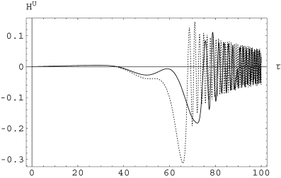
We numerically integrated equations (25)–(35) using the following parameters and initial conditions: ⁠, and 2000 (i.e. magnetic Prandtl number P_m= 1), ξ_i= 1/2 (strong non-linearities) and ξ_i= 1/R_m (weak non-linearities).4 A comment about the chosen values for ξ_i is in order: in principle, this parameter can depend on R_m; however, results of numerical simulations show that it is of the order of unity for R_m < 100. In this sense, the value ξ= 1/2 would be in accordance with those results. As we are working here with larger values of R_m for which, to our knowledge, there is a lack of numerical estimations of ξ_i, we chose two values that might represent the two extreme behaviours of this parameter. Nevertheless, we must stress that the validity of this choice should be checked by direct numerical simulations. In Fig. 1, we plotted as a function of τ for ξ_i= 1/2. The long dashed line corresponds to R_m= 200, while the short dashed one corresponds to R_m= 2000. We see that the generation of is rather weak, but the effect seems to be stronger for R_m= 2000 as time passes. In Fig. 2, we plotted as a function of τ for ξ_i= 1/R_m. The full line corresponds to R_m= 200 while the dotted one corresponds to R_m= 2000. In this case, there is a strong production of large-scale kinetic helicity, it being stronger for R_m= 2000 at the beginning of the integration, while for later times there seems to be no difference between the outcomes for the two R_m considered. In Fig. 3, we plotted the logarithm of the small-scale magnetic energy, ln(Ξ^b₂) as a function of τ, for ξ_i= 1/2. Each curve consists of two curves: one with the effect of and the other without this field. This superposition of curves means that for the chosen value of ξ_i the effect of on the evolution of small-scale magnetic energy is negligible. The upper curve corresponds to the largest value of R_m, and we see that in this case a saturation value for Ξ^b₂ larger than for R_m= 200 is attained. In Fig. 4, we plotted the logarithm of the small-scale magnetic energy ln(Ξ_b) for ξ_i= 1/R_m. Long dashed curves correspond to R_m= 2000: upper curve contains the effect of ⁠, while the lower oscillating curve is without the action of those fields. Short dashed curves correspond to R_m= 200, with the same features for the presence and absence of ⁠. We see that the action of strongly enhances the generation of small-scale magnetic energy, and again this effect is stronger for larger R_m. In Fig. 5, we plotted as a function of τ for ξ_i= 1/2. Here, again each curve consists of two curves, one with the effect of and the other without, showing again that for strong non-linearities the effect of those flows is negligible, consistent with previous figures. The upper curve corresponds to R_m= 2000 while the lower curve corresponds to R_m= 200. We see that again for larger R_m there is an enhancement of ⁠. In Fig. 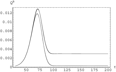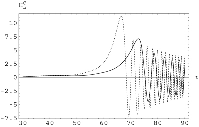6, we plotted as a function of τ for ξ_i= 1/R_m. We see here again that the action of large-scale flows enhances the mean electromotive force ⁠, and this enhancement is stronger for larger R_m. The oscillating, dotted-line curve corresponds to R_m= 2000, and the full-line curve to R_m= 200. The curves corresponding to the absence of the effect of those flows are almost indistinguishable from the τ-axis. In Fig. 7, we plotted as a function of τ for ξ= 1/2. Here, again each curve consists of two curves, one with the effect of and the other without, showing again that for strong non-linearities the effect of those flows is negligible. The fast growing curve corresponds to R_m= 200 while the lower one corresponds to R_m= 2000. The coincidence of the two curves for short times corresponds to the kinematic regime, where back-reaction of the induced magnetic fields b did not take place yet. In Fig. 8, we plotted as a function of τ for ξ= 1/R_m. We see here again that the action of large-scale flows enhances the mean electromotive force and this enhancement is stronger for larger R_m. Dashed curves correspond to R_m= 2000: the ones with the largest amplitude correspond to the action of ⁠, while the lower amplitude corresponds to the absence of this effect. The full line corresponds to R_m= 200 and the features with respect to the presence and absence of large-scale flows are the same as for R_m= 200. The coincidence of all four curves at the beginning of the evolution corresponds to the kinematic regime. In Fig. 9, we plotted as a function of τ for ξ_i= 1/2. The dashed line curve corresponds to R_m= 2000 while the full line corresponds to R_m= 200. Consistently with Fig. 1, we see that is larger for larger R_m. In Fig. 10, we plotted as a function of τ for ξ_i= 1/R_m. The dotted line corresponds to R_m= 2000 while the full corresponds line to R_m= 200. Consistently with Fig. 2, we see that is larger for R_m= 2000 than for R_m= 200, with the difference in amplitudes between both quantities getting smaller with time.

Figure 1

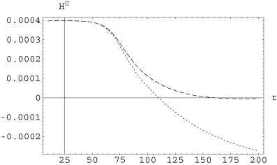
Large-scale kinetic helicity as a function of τ for ξ_i= 1/2. The long dashed line corresponds to R_m= 200, and the dotted line to R_m= 2000. The generation of is stronger for the largest value of R_m.

Open in new tabDownload slide

Figure 2

Large-scale kinetic helicity as a function of τ for ξ_i= 1/R_m. The full line corresponds to R_m= 200, and the dotted one to R_m= 200. At the beginning, the induction of is stronger for the largest value of R_m.

Open in new tabDownload slide

Figure 3

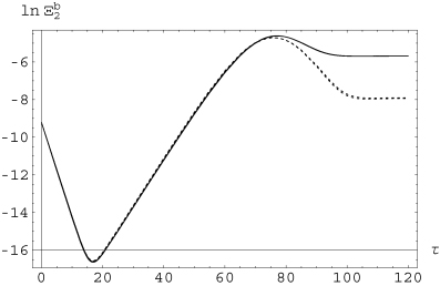
Logarithm of the small-scale magnetic energy Ξ^b₂ as a function of τ, for ξ_i= 1/2. Each curve is in fact two curves, with and without the effect of ⁠, which means that in this case the effect of those flows is negligible. The upper curve corresponds to R_m= 2000 and the lower one to R_m= 200. The small-scale magnetic energy density is very small although larger for R_m= 2000.

Open in new tabDownload slide

Figure 4

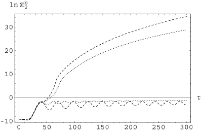
Logarithm of the small-scale magnetic energy Ξ^b₂ as a function of τ for ξ_i= 1/R_m. The upper, long dashed curve corresponds to the presence of ⁠, while the lower, oscillating one corresponds to the absence of those flows, both of them for R_m= 2000. Short dashed curves represent the same quantities but for R_m= 200. In this case, large-scale flows strongly enhance the production of small-scale magnetic energy, and this effect is again stronger for larger values of R_m.

Open in new tabDownload slide

Figure 5

Mean electromotive force as a function of τ for ξ_i= 1/2. Each curve is two curves, one with the effect of and the other without those fields, showing that for this value of ξ the effect of those fields is negligible. The upper curve corresponds to R_m= 2000 and the lower curve to R_m= 200, which shows that for the largest is slightly stronger.

Open in new tabDownload slide

Figure 6

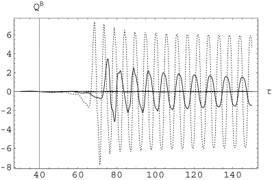
Mean electromotive force as a function of τ for ξ_i= 1/R_m. The dotted line corresponds to R_m= 2000 and the full line to R_m= 200. The curves corresponding to the absence of large-scale flows are of negligible amplitude and almost indistinguishable from the τ-axis, showing that in this case the enhancement of the TEMF by the shear fields is very strong.

Open in new tabDownload slide

Figure 7

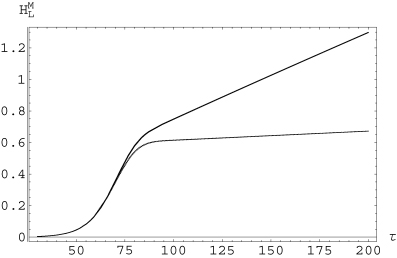
Large-scale magnetic helicity as a function of τ, for ξ_i= 1/2. Again, in this figure, each curve is two curves, one with the effect of and the other without, showing that the effect of those flows on the evolution of magnetic helicity is negligible for the chosen value of ξ_i. The growing curve corresponds to R_m= 200, while the slowly growing, lower curve corresponds to R_m= 2000.

Open in new tabDownload slide

Figure 8

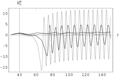
Large-scale magnetic helicity as a function of τ, for ξ_i= 1/R_m. Dotted curves correspond to R_m= 2000, while continuous curves correspond to R_m= 200. In each case, the strongly oscillating curves correspond to the action of large-scale flows, while the slow oscillations correspond to their absence. Consistently with what was shown in Fig. 6, the action of enhances the cascade of magnetic helicity.

Open in new tabDownload slide

Figure 9

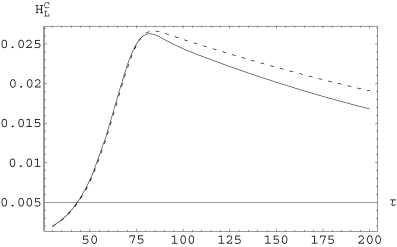
Large-scale cross-helicity as a function of τ for ξ_i= 1/2. Consistently with Fig. 1, the generation of large-scale cross-helicity is stronger for R_m= 2000 (dashed line) than for R_m= 200 (full line).

Open in new tabDownload slide

Figure 10

Large-scale cross-helicity as a function of τ, for ξ_i= 1/R_m. Consistently with Fig. 2, the generation of large-scale cross-helicity is stronger for R_m= 2000 (dotted line) than for R_m= 200 (continuous line).

Open in new tabDownload slide

6 CONCLUSIONS

In this paper, we studied semi-analytically and qualitatively the generation of large-scale flows by the action of a turbulent MFD, and the back-reaction of those flows on the turbulent electromotive force for two values of magnetic Reynolds number, R_m= 200 and 2000, and magnetic Prandtl number P_m= 1. We considered a system in which small-scale turbulent flows are fully helical and prescribed by a given external mechanism, i.e. a kinematically driven dynamo, and that this system possesses boundary conditions such that all total divergencies vanish. The turbulence was considered to be homogeneous and isotropic, which, although being of limited applicability to obtain quantitative results for real systems, serves to study many conceptual aspects of large-scale magnetic field generation, besides enormously simplifying the mathematics. We followed the evolution of large-scale flows through their associated kinetic helicity ⁠, as one of the suppositions we made was that those flows were fully helical too. One crucial assumption we made was that ⁠, which, due to the Coulomb gauge, imposed a further constraint on and that allowed us to express several terms as large-scale cross-helicity. Another one was to assume that is force-free and the main reason to adopt it is that it helped to simplify the mathematics. Although this condition can be fulfilled in certain astrophysical environments, this is not a general situation; therefore it should be dropped off in future works that aim at generalizing this work.

We found that large-scale flows act on the TEMF through large- and small-scale cross-helicities and that for the minimal τ closure considered here, the effect of those fields is stronger for large relaxation times (ξ_i= 1/R_m). For short relaxation time (ξ_i= 1/2), the effect of those fields seems to be negligible. The choice of the values for ξ_i was arbitrary, in the sense that, to our present knowledge, it is not known how that parameter depends on the magnetic Reynolds number for R_m > 100. For R_m < 100, it seems to be confirmed that ξ_i is of the order of unity. Here, we chose to work with two values that may be considered as representative of two extreme possibilities: ξ_i= 1/2 would be consistent with the predictions of the numerical simulations (although they were made for a different R_m interval), while ξ= 1/R_m would represent a resistive case. In any case, more reliable values should be given by numerical simulations performed for R_m > 100.

Due to the simple system considered and the approximations we made, we do not intend to find quantitative results, such as for example estimate the time interval during which is valid, nor do we extract more conceptual and qualitative conclusions. We end this work stressing on the importance of studying this problem via numerical simulations, which will show us the next paths to follow in a further analytical study, besides confirming or contesting the results presented here. The semi-analytical study of the anisotropic case is also of most importance, as well as the consideration of other boundary conditions.

We thank P. Mininni for suggesting the idea of this work and the referee for many suggestions and comments that helped to improve it. Financial support from FAPESB, grant APR205/2005, is acknowledged. The present work was done under project PROPP-UESC 00220.1300.489.

REFERENCES

Appendices

APPENDIX A: DEDUCTION OF THE COMPLEMENTARY EVOLUTION EQUATIONS

Here, we sketch the derivation of the evolution equation for the large-scale kinetic helicity as well as the set of extra equations needed to study the problem considered in this article.

A1 Evolution equation for the large-scale vorticity

We start from the Navier–Stokes equation written in the form

(A1)

The equation for is obtained by simply taking the curl of equation (A1), after replacing the decomposition in mean and stochastic fields, and using the hypothesis that u is fully helical. We have

(A2)

A2 Evolution equation for the large-scale kinetic helicity

It is obtained as ⁠. Replacing the corresponding equations, we obtain

(A3)

where the semi-equality stems from the fact that we approximated ⁠. We define ⁠, and thus equation (A3) reads

(A4)

A3 Evolution equation for and its projections

It is found by taking curl of equation (7) and using it to expand ⁠. After a somewhat lengthy, but straightforward, calculation, where it is assumed that for the two-scale approximation 5 we obtain

(A5)

As in the text, we assume that ⁠, so equation (A5) reduces to

(A6)

To find the evolution equations for the scalar product of with and ⁠, we use the above defined expression ⁠, and an analogous expression for ⁠. Again, the evolution equation is found by taking the time derivative of the complete expression. In the two-scale approximation, we have

(A7)

Due to the fact that ⁠, we can write ⁠. Using the fact that for a fully helical field we can write ⁠, we obtain

(A8)

For the projection of along and along we proceed analogously as for ⁠. Using the fact that for a large-scale force-free field we can write | B₀| =k^1/2_L| H^M_L|^1/2, we obtain

(A9)

and

(A10)

where we used ⁠.

A4 Evolution equation for the cross-helicity

Cross-helicity is defined as H^C=〈U·B〉_vol. After obtaining from equation (A1) the evolution equations for and u and using equation (4) and (7), we obtain the following equation for the large-scale cross-helicity, H^C_L, and the small-scale cross-helicity H^C_S:

(A11)

and

(A12)

Replacing ⁠, defining ⁠, and using the fact that for fully helical we can write ⁠, in the two-scale approximation we have

(A13)

and

(A14)

A5 Evolution equation for

Using equation (12), and ⁠, we obtain

(A15)

where in the last term we considered the term ⁠, and the three-point correlations. Performing ⁠, where the semi-equality before the last stems from the fact that ⁠, we obtain

(A16)

A6 Evolution equation for E^b

It is obtained by scalar multiplying equation (7) by b and then taking volume average. In order to simplify the mathematics, we approximate the volume averages by a dot product between spatial averages of functions of stochastic and mean fields.

(A17)

To deal with the second term we write and thus

(A18)

We obtain for the second term in equation (A17):

(A19)

where the second term in the second row of equation (A18) was considered to give a null contribution when averaged. Defining E^b₂≡ (E^b)², we can write the evolution equation for the small-scale magnetic energy as

(A20)