


Abstract
We present a series of cosmological N-body simulations which make use of the hydrodynamic approach to the evolution of structures. This approach addresses explicitly the existence of a finite spatial resolution and the dynamical effect of subresolution degrees of freedom. We adapt this method to cosmological simulations of the standard Lambda cold dark matter structure formation scenario and study the effects induced at redshift z= 0 by this novel approach on the large-scale clustering patterns as well as (individual) dark matter haloes.
Comparing these simulations to usual N-body simulations, we find that (i) the new (hydrodynamic) model entails a proliferation of low-mass haloes and (ii) dark matter haloes have a higher degree of rotational support. These results agree with the theoretical expectation about the qualitative behaviour of the ‘correction terms’ introduced by the hydrodynamic approach: these terms act as a drain of inflow kinetic energy and a source of vorticity by the small-scale tidal torques and shear stresses.
1 INTRODUCTION
Gravitational instability is commonly accepted as the basic mechanism for structure formation on large scales. Combined with the cold dark matter (CDM) model it leads to the picture of hierarchical clustering with wide support from deep galaxy and cluster observations. During the recent phase of cosmic evolution groups and clusters of galaxies condense from large-scale density enhancements, and they grow by accretion and merger processes of the environmental cosmic matter.
But despite the fact that the currently favoured Lambda CDM (ΛCDM) model has proven to be remarkably successful on large scales (cf. Wilkinson Microwave Anisotropy Probe results, Spergel et al. 2003, 2006), recent high-resolution N-body simulations still seem to be in contradiction with observation on subgalactic scales. There is, for instance, the problem with the steep central densities of galactic haloes as the highest resolution simulations favour a cusp with a logarithmic inner slope for the density profile of approximately −1.2 (Power et al. 2003; Fukushige, Kawai & Makino 2004; Diemand, Moore & Stadel 2005), whereas high-resolution observations of low surface brightness galaxies are best fitted by haloes with a core of constant density (de Block & Bosma 2002; Swaters et al. 2003; Simon et al. 2005). A further problem relates to the overabundance of small-sized (satellite) haloes; there are many more subhaloes predicted by cosmological simulations than actually observed in nearby galaxies (e.g. Moore et al. 1998; Klypin et al. 1999; Gottlöber et al. 2003). The lack of observational evidence for these satellites has led to the suggestion that they are completely (or almost completely) dark, with strongly suppressed star formation due to the removal of gas from the small protogalaxies by the ionizing radiation from the first stars and quasars (Bullock, Kravtsov & Weinberg 2000; Tully et al. 2002; Somerville 2002; Hoeft et al. 2006). Other authors suggest that perhaps low-mass satellites never formed in the predicted numbers in the first place, indicating problems with the ΛCDM model in general, which is replaced with warm dark matter (WDM) instead (Colín, Avila-Reese & Valenzuela 2000; Bode, Ostriker & Turok 2001; Knebe, Green & Binney 2002). Suggested solutions also include the introduction of self-interactions into collisionless N-body simulations (e.g. Bento et al. 2000; Spergel & Steinhardt 2000), and non-standard modifications to an otherwise unperturbed CDM power spectrum (e.g. bumpy power spectra: Little, Knebe & Islam 2003; tilted CDM: Bullock 2001c). Recent results from (strong) lensing statistics though suggest that the predicted excess of substructure is in fact required to reconcile some observations with theory (Dalal & Kochanek 2002; Dahle, Hannestad & Sommer-Larsen 2003), but this conclusion has not been universally accepted (Schechter & Wambsganss 2002; Evans & Witt 2003; Sand et al. 2004).
The discovery of the mismatch between observations and simulations is a result of the increase in the resolution of N-body simulations over the last years. This has emphasized the importance of the influence of subresolution scales on the simulated dynamics, at least when it comes to halo properties. The purpose of this work is to study the hydrodynamic-like formulation of the formation of cosmologial structure proposed recently by Domínguez (2000), dubbed small-size expansion (SSE). The SSE addresses explicitly the existence of a finite spatial resolution and the dynamical effect of subresolution degrees of freedom. Although developed independently, the SSE approach is close in spirit to the large-eddy simulation of turbulent flow (see e.g. Pope 2000, and references therein). This is a method devised to simulate only the relevant, large-scale degrees of freedom according to the Navier–Stokes equations describing flow in the high Reynolds number (i.e. turbulent) regime: physically meaningful approximations are made in order to model the coupling to the neglected, small-scale degrees of freedom.
The SSE starts from the microscopic equations of motion for a set of N particles under their mutual gravity and provides a set of hydrodynamic-like equations for the (coarse-grained) mass density and velocity fields. These new equations now contain ‘correction terms’ which describe the effects of the coarse-graining procedure and correct for them, respectively. It therefore only appears natural to implement these correction terms into an (adaptive) mesh N-body code where the density is treated in a coarse-grained fashion, too: mesh-based Poisson solvers frequently used for cosmological simulations smooth the particle distribution on to a grid and hence deal with a coarse-grained density field when solving for the potential via Poisson's equation. For this purpose we will adapt the open source N-body code mlapm (Multi-Level Adaptive Particle-Mesh).1 The particles of the N-body simulations presented in this study are effectively hydrodynamical Lagrangian particles which move under the action not only of the mesh-computed gravitational force, but also of the additional, correction terms modelling subgrid degrees of freedom in the context of the SSE.
The rest of the work is structured as follows. In Section 2, we describe the theoretical background of the SSE and provide the link to mesh-based N-body codes. In Section 3, we present the simulation of several models (standard ΛCDM model, ΛWDM model, and two runs incorporating the SSE corrections). In Section 4, we perform a comparative analysis of the four runs at redshift z= 0 from two complementary points of view: properties of the mass density and velocity fields, and properties of haloes. Finally, Section 5 includes a discussion of the results and the conclusions.
2 THE HYDRODYNAMIC APPROACH
We deal with a system of non-relativistic, identical point particles which (i) are supposed to interact with each other via gravity only, (ii) look homogeneously distributed on sufficiently large scales, so that the evolution at such scales corresponds to an expanding Friedmann–Lemaıtre cosmological background and (iii) deviations to homogeneity are relevant only on scales small enough that a Newtonian approximation is valid to follow their evolution. Let a(t) then denote the expansion factor of the Friedmann–Lemaıtre cosmological background,  the associated Hubble function, and ϱb(t) the homogeneous (background) density on large scales. xα is the comoving spatial coordinate of the αth particle,
  its peculiar velocity, and m its mass. In terms of these variables the evolution is described by the following set of equations (Peebles 1980) (∇α denotes a partial derivative with respect to xα):


where wα is the peculiar gravitational acceleration acting on the αth particle. Finally, equations (1) must be subjected to periodic boundary conditions in order to yield a Newtonian description consistent with the Friedmann –Lemaıtre solution on large scales (Buchert & Ehlers 1997).
If we now assume that the actual measure of the density field in an N-body code depends on a smoothing window W(z), the microscopic field ϱmic relates to the measured (coarse-grained) field ϱ in the following way:

The physical interpretation of the field ϱ(x; L) follows straightforwardly from the properties of the smoothing window: it is proportional to the number of particles contained within the coarsening cell of size ≈L centred at x. A microscopic peculiar momentum density field and the corresponding coarse-grained field can be defined in the same way:
One can introduce peculiar velocity fields umic and u by definition as j=: ϱu and similarly for umic. The physical meaning of u(x; L) is also simple: it is the centre-of-mass peculiar velocity of the subsystem defined by the particles inside the coarsening cell of size ≈L centred at x. Notice that u is not obtained by coarse-graining umic: from a dynamical point of view, it is more natural to coarse-grain the momentum rather than the velocity, since the former is an additive quantity for a system of particles. Finally, one can define peculiar gravitational acceleration fields wmic and w through coarse-graining of the force:
The field w(x) has the physical meaning of the centre-of-mass peculiar gravitational acceleration of the subsystem defined by the coarsening cell at x.
From these definitions and equations (1), it is straightforward to derive the evolution equations obeyed by the coarse-grained fields ϱ and u (from now on, ∂/∂t is taken at constant x and L, and ∇ means partial derivative with respect to x):
where a new second-rank tensor field has been defined (dyadic notation):
The field π (x) is due to the velocity dispersion, i.e. to the fact that the particles in the coarsening cell have in general a velocity different from that of the centre of mass. The physical meaning of equations (5) is simple: they are just balance equations, stating mass conservation and momentum conservation, respectively. The term ϱw codifies the gravitational interaction between the coarsening cells and does not satisfy, in general, Poisson's equation or the curl-free condition. The term ∇·π represents a kinetic pressure force due to the exchange of particles between neighbouring coarsening cells (just like for an ideal gas) and it has the same physical origin as the convective term ∇· (ϱuu), i.e. a non-linear mode–mode coupling of the velocity field. The difference is that the convective term couples only modes on scales >L, while the velocity dispersion term codifies the dynamical effect of the coupling of the modes on scales >L with the modes on scales <L. Equations (5) are exact: as one changes the smoothing length, the fields ϱ, u, w, π change in such a way that the form of the equations remains the same (e.g. upon increase of the smoothing length, part of the dynamical effect described by ∇· (ϱ uu) is shifted towards ∇·π). This property is reflected in that the equations are not an autonomous system for ϱ and u. In fact, they are just the first ones of an infinite hierarchy, as can be checked by computing the evolution equations for the fields w and π. To obtain a useful set of equations, it is necessary to truncate this hierarchy by looking for a functional dependence of w and π on ϱ and u.
The peculiarities of the problem at hand (collisionless matter in the non-stationary state of structure formation) prevent the usual truncation of the hierarchy leading to the Euler or Navier–Stokes equations, respectively (see e.g. Chapman & Cowling 1991). The SSE is a specific truncation for this problem (Domínguez 2000, 2002; Buchert & Domínguez 2005), that starts from the physical assumption that the coupling to the small scales is weak (this can be argued on the basis that, in a hierarchical scenario, the smaller scales ‘virialize’ earlier and thus ‘decouple’ from the evolution of the larger scales). Then the fields π and w are derived as a formal expansion in L: keeping terms up to order L2, equations (5) become (∂i=∂/∂xi; summation over the repeated index i is understood)

with the additional acceleration
The constant B is determined by the smoothing window W(z),
To order L0, equations (7) reduce to the ‘dust (pressureless) approximation’ for cosmological structure formation (Sahni & Coles 1995): wmf represents the mean-field gravity created by the monopole moment of the matter distribution in the coarsening cells, i.e. the total mass, and the coupling to the small scales is neglected altogether. To order L2 there are two kinds of corrections: the term proportional to the tidal tensor ∇wmf, stemming from a term w−wmf in equations (5), models the gravitational force of the higher order multipole moments, i.e. the coupling to the subresolution configurational degrees of freedom; the term proportional to (∂iu) (∂iu), stemming from π in equations (5) models the effect of velocity dispersion, i.e. the coupling to the subresolution kinetic degrees of freedom.
The expected dynamical effect of these new terms with respect to the ‘dust evolution’ has been studied theoretically (Domínguez 2000, 2002; Buchert & Domínguez 2005). There is evidence that, assuming a locally plane-parallel collapse, these terms mimick the ‘adhesion model’ (Gurbatov, Saichev & Shandarin 1989; Sahni & Coles 1995), in which recently collapsed regions stabilize – or more generally speaking, the term due to velocity dispersion tends to reduce the inflow velocity in collapsing regions and favours the formation of gravitationally bound systems. It has also been shown that the correction terms act as a source of vorticity via small-scale tidal forces and shear stresses. The ‘dust model’ lacks a source of vorticity ω=∇×u, and the initially present one is damped by the cosmological expansion in the linear regime. Thus, in that respect the corrections to the ‘dust model’ can be particularly important. Taking the curl of equation (7b) we obtain
where the term ∇×C is a source of vorticity, i.e. it does not vanish in general even if ω=0, as has been confirmed perturbatively by Domínguez (2002). We comment further on the relationship between vorticity and angular momentum in Appendix A, where also some results concerning the conservation of energy, momentum and angular momentum are derived.
The dynamical evolution predicted by equations (7) can be implemented without much difficulties in a particle-mesh (PM) code of N-body simulation. Mass conservation, equation (7a), is automatically satisfied by the code. The acceleration wmf given by equations (7c) and (7d) agrees with the value returned by the Poisson solver on a grid, and the grid constant sets naturally the resolution L. In principle, one only needs to take care of equation (7b), which can be rewritten in Lagrangian coordinates as
The computation of C, given by equation (8), on the grid of the Poisson solver is a highly non-trivial but manageable task. Thus, equation (11)– together with  , see equation (1a)– determines the motion of Lagrangian fluid elements, which are sampled by the particles of the simulation. If we set B= 0 (⇒C=0) in equation (11) we recover the equations of motions that are being integrated in a standard PM code for the update of particle velocities and positions during the course of the simulation.
3 THE N-BODY SIMULATIONS
3.1 The set-up
The N-body simulations presented in this study were carried out using a version of the open source adaptive mesh refinement code mlapm (Knebe et al. 2001). This code reaches high force resolution by refining high-density regions with an automated refinement algorithm. These adaptive meshes are recursive: refined regions can also be refined, each subsequent refinement having cells that are half the size of the cells in the previous level. This creates a hierarchy of refinement meshes of different resolutions covering regions of interest. The refinement is done cell by cell (individual cells can be refined or de-refined) and meshes are not constrained to have a rectangular (or any other) shape. The criterion for (de-)refining a cell is simply the number of particles within that cell and a detailed study of the appropriate choice for this number can be found elsewhere (Knebe et al. 2001). The code also uses multiple time-steps on different refinement levels where the time-step for each level is two times smaller than the step on the previous level. The latest version of mlapm also includes an adaptive time-stepping that adjusts the actual time-step after every major step to restrict particle movement across a cell to a particular fraction of the cell spacing, hence, fine tuning accuracy and computational time.
As outlined above, the only necessary modification required to model the ‘Hydrodynamic APProxImation’ (or ‘HAPPI’ hereafter) is to account for the correction term C in equation (11) when updating the particle velocities.2mlapm has therefore been modified to not only calculate the density field on its hierarchy of nested refinement grids but also the velocity field. The ∇-operator and spatial derivatives, respectively, have been approximated by finite differences using the two nearest neighbours (in each dimension) to the cell for which the correction term is being calculated. Cells close to a refinement boundary for which not enough surrounding nodes are present, obtain their correction values interpolated downwards from the next coarser grid level. The assignment of mass and momentum on the grid is done with a triangular-shaped-cloud window (Hockney & Eastwood 1988),
for which B= 1/4 according to equation (9). We remark that, due to the dynamical (de)refinement procedure of the mlapm code, the resolution is space dependent in a discrete manner, while equations (7) were derived under the assumption of a spatially homogeneous length L. The SSE can be generalized to the case of a smoothly varying L(x) [Domínguez (unpublished); Domínguez (2002) contains the generalization to a time-dependent L], but we have neglected this additional complication because the fraction of particles which are in regions where L jumps is less than 1 per cent during the run. Finally, we also note that this numerical method of integrating the hydrodynamic equations is different from, albeit similar to, the smoothed particle hydrodynamics method (Gingold & Monaghan 1977; Lucy 1977) frequently used in cosmological simulations involving baryonic matter.
We ran four simulations with cosmological parameters in agreement with the so-called concordance model, i.e. Ω0= 1/3, λ0= 2/3, σ8= 0.88, h= 2/3:
one standard ΛCDM model,
one ΛWDM model (mWDM= 0.5 keV),
two ΛCDM models with B= 1/4 and B= 1, respectively.
Even though B is actually determined by the smoothing window, we also considered a four times larger value as if it were a free parameter of the model. This model is to be understood as an ‘academic toy model’ where we hope to gain better insight into the effects of the correction term on cosmological structure formation.
All simulations consist of N= 1283 particles in a box of side length 25 h−1 Mpc (the mass of a simulation particle is mpart≈ 7 × 10⁸h−1 M⊙), and they were started at redshift z= 35. The two ΛCDM models with B≠ 0 are also dubbed ΛCDM happi1 (B= 1/4) and ΛCDM happi2 (B= 1). We chose to also run a ΛWDM model to allow for a more complete comparison of the new HAPPI models to other, alternative cosmologies. A more elaborate study of the ΛWDM model and WDM can be found in Knebe et al. (2002).
The force resolution in mlapm is determined by the finest refinement level reached throughout the run. While all four models applied exactly the same refinement criterion (six particles per cell), the ΛCDM happi2 run only invoked five refinement levels whereas all other runs used seven levels at redshift z= 0. In terms of force resolution this translates to 10 h−1 kpc spatial resolution for ΛCDM happi2 (corresponding to an estimated maximum density ∼5 × 10⁴ϱb) and 2.5 h−1 kpc for all the other models (maximum density ∼3 × 10⁶ϱb). This difference can be ascribed to the smoothening effect of the correction terms in the dynamical equations that are more effective for higher values of B.
3.2 Accuracy of the code
A useful check of the accuracy of a simulation is provided by the global invariants of the dynamical system, which we derive and discuss in Appendix A.
The dynamical evolution conserves the quantity  (if the force and density interpolation schemes are identical). It was found that departures from the initially vanishing value satisfy the bound
where at redshift z= 0 the average particle velocity was umean≈ 300 km s−1 in all four models.
In standard N-body codes it is common practice to check constancy of the invariant  (see equation A5) following from the Layzer–Irvine equation (e.g. Knebe et al. 2001). This is not the case for the two HAPPI models, since the correction term C is a source or drain of energy as discussed in Appendix A. We though chose to plot in Fig. 1 the dimensionless quantity
as a function of cosmic expansion factor a, where Umf is the mean-field potential energy defined in equations (A1). For the ΛCDM and ΛWDM models, the Layzer–Irvine equation holds and predicts  . Departures from this result are ascribed to both integration/truncation errors introduced by the code and the fact that the particle shape is neither constant in time nor space due to the adaptive nature of mlapm (cf. Knebe et al. 2001). ΛCDM happi1 performs rather similar to the standard CDM model, indicating that the effect of the correction term C in the evolution of
  is small compared to the numerical errors. ΛCDM happi2, on the other hand, departs noticeably from the other models and
  changes sign at around a redshift of z≈ 3, which lets us expect to find larger differences between ΛCDM happi2 and ΛCDM.
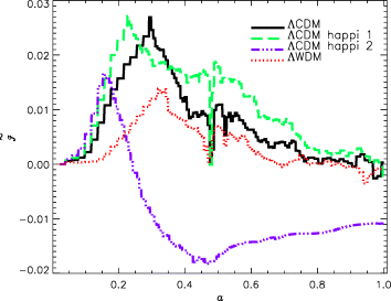
Variation with the expansion factor a of the dimensionless quantity  defined by equation (14).
3.3 The Importance of the HAPPI correction
In order to test the importance of the correction term equation (8) we calculated the ratio of the mean-field acceleration (i.e. F= |wmf|) and the additional acceleration (C= |C|) for each individual particle as a function of the local density at various redshifts. The result for the ΛCDM happi2 model, for which the effect of C is the largest, can be viewed in Fig. 2. This figure indicates that the effect of the newly added terms is generally rather small especially at late times. At redshift z= 0 the fraction of all particles with F/C < 1 (‘HAPPI particles’) is a mere 9 per cent while it increases to 15 per cent at z= 4. In order to examine a possible trend with density, we consider at each redshift two subsets of particles according to whether the density is above or below the virial overdensity Δvir (cf. equation 17 in Section 4.2) and hence particles of the high-density subset either already belong to virialized structures or will be part of them at a later time. Table 1 gives the fraction of HAPPI particles in each subset.
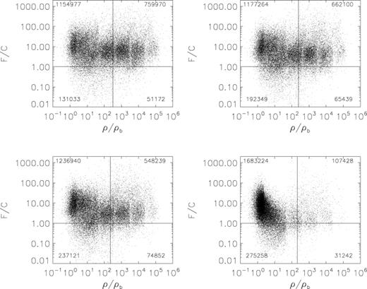
The correction term in comparison to the mean-field force acting on a single particle as a function of density. The four panels are for all particles in the simulation at redshifts z= 0 (upper left-hand panel), z= 0.5 (upper right-hand panel), z= 1.0 (lower left-hand panel) and z= 4.0 (lower right-hand panel). The vertical line indicates the virial overdensity at the respective redshift. The number in each quadrant lists the total number of particles in this regime of the plot.
Fraction of HAPPI particles in the subset of low-density particles, and in the subset of high-density particles, respectively.
| Redshift (z) | Low density (per cent) | High density (per cent) |
|---|---|---|
| 0 | 10 | 6 |
| 0.5 | 14 | 9 |
| 1 | 16 | 12 |
| 4 | 14 | 23 |
| Redshift (z) | Low density (per cent) | High density (per cent) |
|---|---|---|
| 0 | 10 | 6 |
| 0.5 | 14 | 9 |
| 1 | 16 | 12 |
| 4 | 14 | 23 |
This raises the question about the exact locations as well as the ‘dynamics’ of HAPPI particles. A visual inspection shows that, at high redshift, they are preferentially located within the filaments flowing towards haloes. At later times though, they can be found either in regions of strong dynamical activity (e.g. mergers, the outskirts of haloes and infall to haloes), or at the very centres of relaxed systems. The smaller spatial force resolution of the ΛCDM happi2 mentioned earlier can hence be linked to the influence of the HAPPI particles at the very centres of haloes.
4 ANALYSIS OF THE MATTER DISTRIBUTION
4.1 Large-scale structure and global properties
A visual impression of the density field of the particle distribution at redshift z= 0 for all four models is shown in Fig. 3, where the local density at each particle position was determined by smoothing the distribution on to a regular grid (2563 nodes) and interpolating the density on the mesh back to the particle positions. Not surprisingly, the ΛWDM model appears less clumpy and far smoother than the ΛCDM simulation. However, there appears to be more small-scale structure in both the HAPPI runs, or at least the smaller objects are more contrasted. We can readily relate this phenomenon to the influence of B and larger B values give higher contrasts (remember that the fiducial ΛCDM model is nothing else than a HAPPI model with B= 0). But despite the more grainy appearance of the HAPPI runs in Fig. 3, the power on small scales is reduced compared to the power of the ΛCDM model. This can be verified in Fig. 4, where we plot the dark matter power spectrum of density fluctuations for all four models at redshifts z= 3 (lower curves) and z= 0 (upper curves). Especially ΛCDM happi2 falls behind ΛCDM even though it appears to be marginally more evolved at higher redshift. We will though see that these two results, the ‘graininess’ of the ΛCDM happi2 model and the lack of small-scale power, do not exclude each other. The absence of small-scale power on scales below ∼1–2 h−1 Mpc reflects the fact that the haloes corresponding to those scales (i.e. haloes of mass >1011h−1 M⊙) are internally less concentrated than their ΛCDM counterparts.
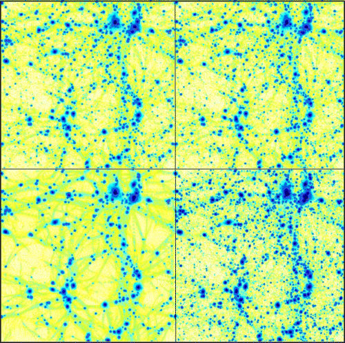
Colour-coded density field of all four models at redshift z= 0. The order is (clockwise starting upper left-hand panel) ΛCDM, ΛCDM happi1, ΛCDM happi2, and ΛWDM.
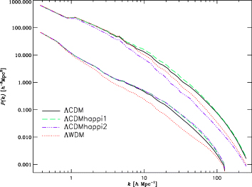
Dark matter power spectrum P(k) for all models at redshifts z= 3 (lower curves) and z= 0 (upper curves).
4.1.1 Beyond the two-point estimators
Two-point estimators like the power spectrum are sensitive only to the amplitude of the modes of the fluctuating field ϱ(x) −ϱb. The information concerning the relative phases is contained in the higher order correlations. In the literature there have been several meaningful quantities proposed depending on higher order correlations with a more or less transparent physical interpretation. In this work, we have employed the scalar Minkowski functionals (MFs) (see e.g. Mecke & Stoyan 2000; Domínguez 2001), which allow a quantification of the morphological aspects appreciated by visual inspections. Given a density field ϱ(x) and a density threshold  , one constructs the isodensity surface
  (with the convention that the region
  is taken as the interior of
  ). The four MFs Vν, ν= 0, 1, 2, 3, can be defined as surface integrals over
  and have the following geometrical meaning (up to a conventional constant prefactor):
V0 is in fact proportional to the probability that  (assuming spatial ergodicity of the realization). The ratio V1/V0 is a measure of how compact the volume enclosed by
  is packed. V2/V1 is a measure of the convexity of the surface
  , while V3 is proportional to the Euler characteristic or genus of the body defined by
  :
:
There seems to be a close relation between the threshold value at which V3 vanishes and the percolation threshold of the volume enclosed by  (Mecke & Wagner 1991; Neher 2003) – as a matter of fact, the use of percolation analysis is not rare in the analysis of cosmological structures (e.g. Yess & Shandarin 1996). As an example of how the MFs are to be interpreted, in Appendix B we discuss the case that ϱ(x) is derived from a realization of a Poissonian distribution of points.
Starting from the positions of the particles given by the simulation, a density field ϱ(x) is generated on a grid by smoothing with the window equation (12). We generated 20 different realizations of the field by displacing randomly the grid and we present the MFs averaged over these realizations. The MFs are functions of the grid constant and the density threshold. We observe that the measurement of the MFs in an N-body simulation is affected by two kinds of errors (which are more pronounced for higher orders ν of the MF Vν).
Finite-volume effects: The tails of the probability distribution of the density field cannot be probed correctly in a finite volume, so that the measured MFs are noisy and take discrete values (due to the grid) as the threshold approaches the extremal values probed in a given simulation. This effect can be reduced by increasing the number of realizations.
Finite-mass effects: At threshold values corresponding to ≲1–10 particles per grid node, the MFs detect that the density field is actually derived from a distribution of point particles.
In order to emphasize the differences between the four simulations and to facilitate the physical interpretation, we plotted as a function of  the relative difference between a measure in one model and the corresponding one in the reference ΛCDM model (denoted by ‘ref’):
The plots are shown in Fig. 5 for a grid of 1283 nodes. As a general feature, the trend of the ΛWDM model with respect to the reference ΛCDM model is always opposite to the trend of the two HAPPI runs, with the deviations of ΛCDM happi2 being larger than those of ΛCDM happi1. Only at very high density thresholds, ΛCDM happi2 seems to follow an opposite trend to ΛCDM happi1: this is because the maximum density in the ΛCDM happi2 run is smaller than in the ΛCDM happi1 or ΛCDM runs. This (physical) effect has been already noticed concerning the final force resolution of the runs: it is due to the larger effect of the additional acceleration C and can be directly linked to the location of ‘HAPPI particles’ at redshift z= 0 at the centre of relaxed structures, see Sections 3.1 and 3.3. The results can be summarized as follows.
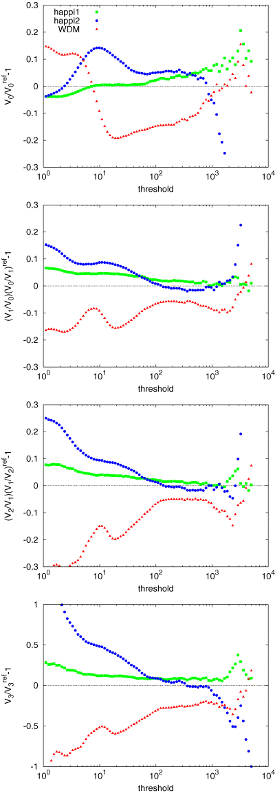
MFs versus density threshold at redshift z= 0. The threshold is given in units of particles per grid node. The grid has 1283 nodes, corresponding to a grid constant 0.20 h−1 Mpc, so that the threshold coincides with the ratio ϱ/ϱb for this spatial resolution.
The dependence
 quantifies the visual impression that low-density regions (ϱ≲ 10 ϱb) are clearly less likely in the WDM model, while overdense regions (10 ≲ϱ/ϱb≲ 103) are more abundant in the HAPPI models. As remarked, higher density areas are rarer in ΛCDM happi2 and more frequent in ΛCDM happi1 compared to ΛCDM.
From the fact that V2, V3 > 0 (not shown in the plot) in the whole range of threshold values, one infers that, observed at the resolution of 1283 nodes, the matter distribution consists mainly of ‘clusters’ (i.e. disconnected objects which are convex on average). According to the plot of
 , these clusters in the HAPPI runs tend to be rounder than in the ΛCDM run, while they tend to be more cigar-shaped (filament-like) in the ΛWDM model. From the plot of
  one deduces that the ΛWDM model has less clusters at all threshold values; the HAPPI runs have more clusters, except for ΛCDM happi2 at very high densities because this particular model does not reach as high densities as the other ones.
Finally, the plot of
 shows that matter is more compactly packed in the ΛWDM model, and less compactly in the HAPPI runs. This is likely due to the different cluster abundances just discussed.
We have repeated the analysis at different spatial resolutions (163, 323, 643 and 2563 nodes) for the MFs. The quantitative differences between models decrease as the grid becomes coarser, but the same conclusions hold roughly in a qualitative manner.
Summarizing, the ΛWDM run has less voids and more filamentary-like structures than the reference ΛCDM model, while the HAPPI runs have comparatively more mass concentrated in small, roundish clusters.
4.1.2 The velocity field
Motivated by the theoretical discussion, we have also addressed the distribution of the (comoving) vorticity, ω=∇×u, and the (comoving) divergence, θ=∇·u, of the peculiar velocity field u(x). Using the positions and velocities of the particles, we compute the fields ω(x) and θ(x) on a regular grid (see Section 3). The cumulative probabilities that  and that
  are given by the first MF V0, which we compute as explained previously.
Fig. 6 shows P/Pref− 1, where P is the cumulative probability measured in a simulation, and Pref is the corresponding probability in the reference ΛCDM simulation. The ΛCDM happi2 model shows a clear tendency to have a larger vorticity and a lower divergence (in absolute value) than the ΛCDM model. The vorticity in the ΛCDM happi1 model exhibits a similar tendency, but the differences are quantitatively smaller. In order to minimize finite-mass effects, we considered only grid nodes for which the value of the smoothed density field corresponds to more than 10 particle per node. If we restrict the measurement of the probability distributions to higher densities, the quantitative differences tend to be smaller.
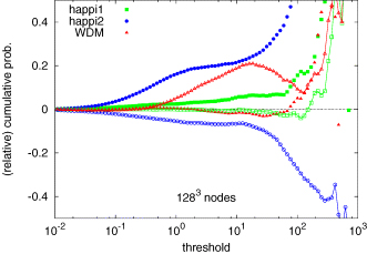
Cumulative probabilities  relative to the probabilities in the ΛCDM model at redshift z= 0 at a resolution of 1283 grid nodes. The solid symbols represent the (relative) cumulative probability of the vorticity, the joined open symbols correspond to the divergence. The threshold
  is given in units of H20.
4.2 Dark matter haloes
The analysis in the following Subsection is primarily based upon gravitational bound objects which were identified using mlapm's Halo Finder (MHF) (Gill, Knebe & Gibson 2004). This newly developed halo finder uses the adaptive grid structure invoked by the N-body code mlapm and re-organizes it into a tree. The centres of the grids at the end-leaves of a branch of the tree serve as (potential) halo centres and all gravitationally bound particles about these centres are being collected. For a more elaborate discussion of this halo finder we refer the reader to Gill et al. (2004). We only like to note at this point that MHF is essentially parameter free and naturally finds haloes with exactly the same accuracy as the simulation. Besides of the growth of the halo mass function and the abundance evolution of gravitationally bound objects, respectively, we confine our analysis to objects identified at redshift z= 0. The investigation of the evolutionary history and hierarchical growth of structures will be published elsewhere.
4.2.1 Global properties
In Fig. 7, we show the evolution of the cumulative mass function n(>M) of dark matter haloes, i.e. the number of DM haloes with mass larger than M. The ΛWDM model clearly has less low-mass objects as already pointed out by other authors (Colín et al. 2000; Bode et al. 2001; Knebe et al. 2002). All three CDM models though perfectly agree at a redshift of z= 5, but there is a clear trend for the HAPPI models to give rise to more small mass haloes, in agreement with the conclusion derived in the previous section. This can be verified in Fig. 8, where we plot the number density evolution of objects more massive than M > 1010h−1 M⊙ (>20 particles). In ΛCDM happi2 there are roughly 50 per cent more haloes above our mass cut than in the reference ΛCDM run.
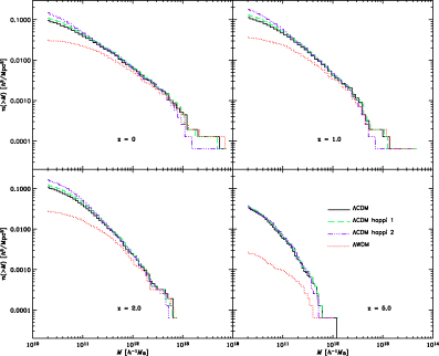
Cumulative mass function n(>M) of DM haloes.
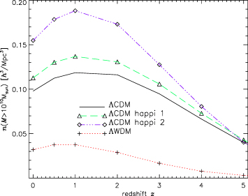
Number density evolution of objects more massive than M > 1010h−1 M⊙.
In order to study the clustering properties of these haloes we estimated the two-point correlation function for low- and high-mass objects, respectively, as
where Ngal is the total number of objects in the simulation volume V, and nα(r; Δr) is the total number of objects in a spherical shell of radius r and thickness Δr[and volume v(r; Δr)], centred at the αth object. The result (along with Poisson error bars based upon the number of pairs in each bin) is shown in Fig. 9. The low-mass objects show very similar clustering patterns, with a higher amplitude of ξgal for ΛWDM and a marginally decreased correlation for the ΛCDM happi2 model. The situation though is difficult to judge at the high-mass end as we have too few pairs per bin to make conclusive statements. The errors bars are larger than the differences amongst the models and hence have been omitted. It seems, however, that the clustering pattern of high mass objects is similar in all models and does not show differences when including the HAPPI correction term.
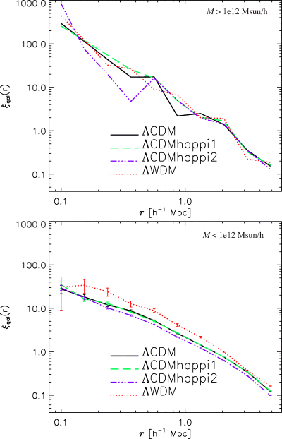
Two-point correlation function of objects more massive (upper panel) and less massive (lower panel) than 1012h−1 M⊙.
The most striking (and interesting) difference between standard ΛCDM and the two HAPPI models, however, emerges when we turn to the spin parameter distribution. The spin parameter λ was calculated using the definition given by Bullock et al. (2001a),
where L is the angular momentum of the halo with respect to its centre of mass, rvir is the virial radius of the halo, Mvir is the virial mass (mass enclosed within the virial radius), and  is the circular velocity at the virial radius. The virial radius and mass are determined by the condition
where ϱvir=Δvirϱb(z= 0) is a fiducial density with Δvir≈ 340 (at redshift z= 0) based on the dissipationless spherical top-hat collapse model for the cosmological parameters of the ΛCDM model. The probability distribution, P(λ), of the spin parameter was fitted to a lognormal distribution (e.g. Frenk et al. 1988; Warren et al. 1992; Cole & Lacey 1996; Gardner 2001; Maller, Dekel & Somerville 2002),
The results are presented in Fig. 10 and in Table 2, showing that a larger value of B entails a larger spin parameter. In the lower panel of Fig. 10– where we plot the cumulative distribution of the spin parameter – we clearly see that for a given λ the probability to find haloes with a smallerλ is greatly lowered in ΛCDM happi2 – or in other words, it is more likely to find haloes with larger spin parameters in ΛCDM happi2. As we will see later on (cf. Fig. 13 in Section 4.2.2), there is a mass dependence of this result: lower mass haloes tend to dominate the signal seen in Fig. 10. When plotting the mass-weighted spin parameter distribution (not shown) the peaks for all four models approach each other. However, even then the HAPPI runs still show a distinct tail out to larger λ values.
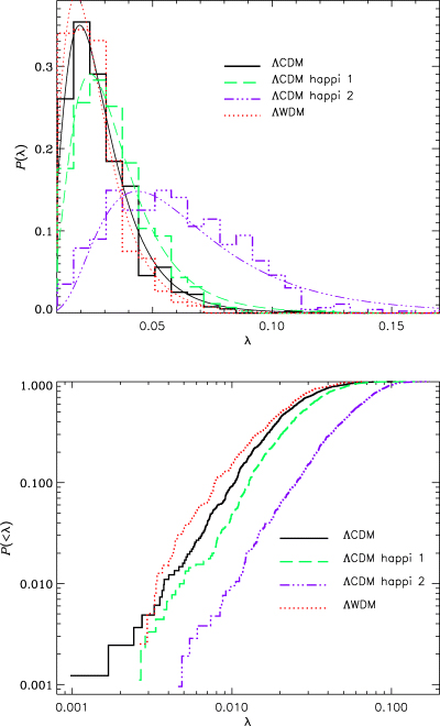
Upper plot: measured spin parameter distribution for all four models at redshift z= 0, and the corresponding fit to equation (18). Lower plot: measured cumulative distribution of the spin parameter.
Parameters derived from fitting the spin parameter distributions P(λ) to equation (18).
| Model | λ0 | σ0 |
|---|---|---|
| ΛCDM | 0.0287 | 0.4485 |
| ΛCDM happi1 | 0.0333 | 0.4611 |
| ΛCDM happi2 | 0.0596 | 0.4914 |
| ΛWDM | 0.0259 | 0.4001 |
| Model | λ0 | σ0 |
|---|---|---|
| ΛCDM | 0.0287 | 0.4485 |
| ΛCDM happi1 | 0.0333 | 0.4611 |
| ΛCDM happi2 | 0.0596 | 0.4914 |
| ΛWDM | 0.0259 | 0.4001 |
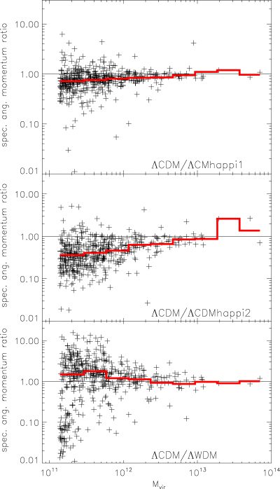
Ratio of specific angular momenta.
The HAPPI correction term also affects the concentration of dark matter haloes. We define the concentration c1/5 as the ratio of the virial radius rvir and the radius of the sphere that contains 1/5 of the virial mass [i.e. r1/5 is defined via M(< r1/5) =Mvir/5]:

In view of definition (17), it follows that the average density within a radius r1/5 is given by (1/5) c31/5ϱvir. Fig. 11 plots the cumulative probability distribution of the concentration of haloes. We observe an obvious trend for an overabundance of low-concentration haloes in the ΛWDM and ΛCDM happi2 models. However, the opposite actually holds for ΛCDM happi1, where there appear to be of order 10 per cent more concentrated haloes. The relative lack of power on scales ≲1 h−1 Mpc noted in Fig. 4 for WDM and ΛCDM happi2 is related to the relatively lower concentration (and increased smoothness for WDM) of the haloes observed in these models (one must bear in mind that the haloes have a virial radius ≲800 h−1 kpc, see Fig. 16).
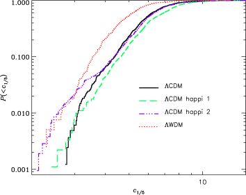
Cumulative distribution of the concentration parameter c1/5.
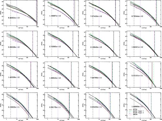
Density profiles for haloes at redshift z= 0. The number printed into each halo panel is the mass of the halo in units of h−1 M⊙. The vertical lines to the right-hand side indicate the respective virial radius while the two vertical lines to the left-hand side indicate the spatial resolution of the ΛCDM, ΛCDM happi1, ΛWDM (dashed line) and ΛCDM happi2 (dotted line) run, respectively.
Although not shown, we confirm that the scaling of the concentration c1/5, defined by equation (19), with mass Mvir follows the same relation as the one proposed by Bullock et al. (2001b) for the ‘NFW (Navarro, Frenk & White) concentration’ of the halo, cNFW=rvir/rs (see equation 21 for the definition of rs).
4.2.2 Cross-correlations
While the last section dealt with the distribution of halo properties, we now compare these properties across the models, i.e. how do these properties change in a given halo when moving from one model to another?
In order to find corresponding haloes across the four models, we compare their individual particle content. We start with a halo in the ΛCDM model, whose particles are tagged, and locate the corresponding halo in the other three models as the one that shares the largest number of tagged particles. In Figs 12–14, we always plot the value of the property under investigation in the ΛCDM model, divided by the value of said property in the other model for all ‘cross-identified’ haloes. These ‘scatter-plots’ are always accompanied by histograms, where we average the ratios presented in the respective figure in nine bins across the actual mass range. The percentages of counterparts amount to practically 100 per cent for the HAPPI models while there are only 40 per cent cross-identified haloes in the ΛWDM model. This number though increases to about 90 per cent when we consider haloes containing more than 200 particles (i.e. M≳ 1011h−1 M⊙), and hence we set this as a lower limit in the cross-correlation plots.
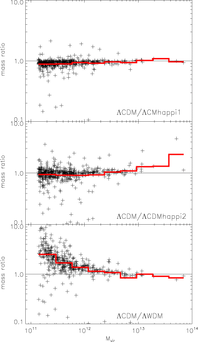
Ratio of halo masses for cross-identified objects. The virial mass Mvir is given in units of h−1 M⊙. The histograms represent the mean ratio in the respective bin.
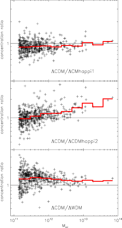
Ratio of halo concentrations c1/5.
We start with the most obvious halo attribute, namely the halo mass itself. Fig. 12 shows that there is a very tight correlation for the masses of individual haloes, especially for ΛCDM and ΛCDM happi1. The scatter about the 1:1 relation (the flat line of value 1) marginally increases from ∼11 per cent (averaged 1σ-value) for ΛCDM happi1 to ∼18 per cent for ΛCDM happi2. At the high-mass end, the ΛCDM happi2 haloes tend to have a slightly larger mass. The most pronounced differences can be found for ΛWDM though: at the low-mass end the haloes in ΛWDM appear to be less massive than their ΛCDM counter parts.
In the previous section we showed that the HAPPI correction term lead to an increase in angular momentum by investigating the spin parameter distributions. But can we be sure that the observed rise in λ as defined by equation (16) is not related to a possible decrease of virial radius rvir and/or virial velocity vvir? To clarify this uncertainty we show in Fig. 13 the cross-correlation of total specific angular momentum,

In view of the already mentioned minimal scatter in the mass of cross-identified haloes between the ΛCDM model and the HAPPI models, Fig. 13 confirms the previous result that one effect of the term C in equation (7b) is to inject angular momentum to haloes. We also note that there is a mass dependence in this trend: the differences in angular momentum are on average larger for lower mass objects, this being particularly noticeable for the ΛCDM happi2 and ΛWDM models; this ‘break’ roughly happens at around 1012h−1 M⊙.
We close this section with an investigation of the cross-correlation of the concentration parameter c1/5 in Fig. 14. The results are consistent with Fig. 11: ΛCDM happi1 haloes are more concentrated than their ΛCDM counterparts, while the excess of low-concentration haloes for ΛCDM happi2 is due to high-mass haloes. The mass trend already noted in Fig. 13 can also be acknowledged in this figure.
Finally, we mention as a general property that the dispersion in the scatter plots increases as the halo mass diminishes. We attribute most of this scatter to differences in the halo's formation history, but a detailed study as function of redshift is required which we will postpone to a later paper. Moreover, numerical effects could also contribute to some extent.
4.2.3 A closer view of individual haloes
A visual representation of the two most massive haloes in all four models is given in Fig. 15. This figure nicely demonstrates the result regarding the lower concentrations in (high-mass) ΛCDM happi2 haloes: the second most massive halo does not even show a distinct centre in ΛCDM happi2 and appears more ‘puffy’ than in any of the other models.
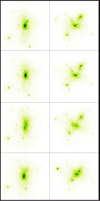
Visual representation of the two most massive haloes at redshift z= 0. The left-hand column shows the most massive halo while the right-hand column is the second most massive one. From top to bottom one has ΛCDM, ΛCDM happi1, ΛCDM happi2 and ΛWDM.
The question now arises whether the density profiles of the HAPPI models can still be fitted by the universal density profile advocated by Navarro, Frenk & White (1997)
Fig. 16 now shows ρ(r) and the corresponding best fits to NFW profiles for a selection of haloes covering the mass range from the most massive one (upper left-hand panel) to rather light haloes (lower right-hand panel) containing a mere 300 particles. For (nearly) all ΛCDM happi2 haloes we observe a relative flattening in the central regions.
In order to gauge the quality of the fits (for the 16 presented sample profiles) we calculate the χ2 value defined as
where ρi are the binned density profiles derived from the simulation data and ρNFW the best-fitting NFW profiles. This analysis then indicates that all four models are equally well fitted by equation (21) with χ2 varying in the range χ2∼ 0.02–0.05 depending on the weighing scheme applied for each individual bin. This entails that the dark matter haloes of the HAPPI runs still exhibit the rather infamous ‘cusp’ at the centre.
We remind the reader again that the force resolution throughout the runs varies. Whereas ΛCDM, ΛCDM happi1 and ΛWDM reached 2.5 h−1 kpc resolution, ΛCDM happi2 reliably resolves structures only on scales larger than 10 h−1 kpc. Moreover, the resolution can also change from halo to halo due to the adaptive mesh nature of both the halo finder and the N-body code: not all halo centres lie on the finest grid level reached in the simulation. However, we plot profiles starting from the distance rmin that corresponds to a sphere containing at least 10 particles (and hence rmin can be actually smaller than the nominal resolution of the simulation).
For the same set of haloes we present in Fig. 17 the rotation curves out to half the respective virial radius. The rotational velocity vcirc(r) is defined as
There are a number of interesting observations to discuss now. We find that in nearly every halo the ΛCDM happi1 rotation curve rises to higher values than any of the other models. While the maximum is still at comparable distances in ΛCDM and ΛCDM happi1, the latter shows a steeper inner increase and a subsequent faster decline to nearly the same level in the ‘outer’ parts. Moreover, the ΛCDM happi1 rotation curves are always slightly above the corresponding ΛCDM curves. Quite the opposite is true for ΛCDM happi2. Here, we find that in most of the cases the circular rotation values at a given radius are substantially smaller than in ΛCDM. However, this difference becomes less prominent in lower mass systems and the flat part of the rotation curve nearly reaches the same level as ΛCDM. This discrepancy in the trends between ΛCDM happi1 and ΛCDM happi2 for high-mass haloes is likely related to the also opposite trends concerning the concentration, Figs 11 and 14, and the small-scale power, Fig. 4.
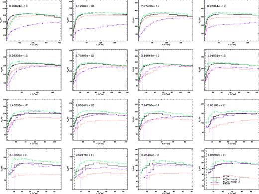
Rotation curves for the same haloes as in Fig. 16.
5 DISCUSSION AND CONCLUSIONS
We have presented a series of cosmological N-body simulations which made use of the hydrodynamic approach to the evolution of structures (Domínguez 2000). This approach is novel in that it deals with the mass density and velocity fields with explicit account of the coarse-grained nature intrinsic to any approach of solving, for instance, Poisson's equation via Monte Carlo sampling of phase space. This N-body approach unavoidably introduces finite-resolution effects and there have been systematic studies of the consequences in the context of cosmological structure formation (Kuhlman, Melott & Shandarin 1996; Moore et al. 1998; Splinter et al. 1998; Knebe et al. 2000; Power et al. 2003). N-body simulations invariably neglect the dynamical effect of subresolution degrees of freedom altogether. For the first time, we have run simulations including a physical model of the coupling to the neglected scales. N-body codes are usually viewed as integrators of the Vlasov–Poisson system of equations. However, we have argued how grid-based N-body codes such as mlapm can be reinterpreted to integrate hydrodynamic-like equations for the mass density and velocity fields.
The additional, correction term introduced in the hydrodynamic approach is proportional to a ‘coupling constant’B which depends on the smoothing window used to calculate the coarse-grained fields. It is found to be B= 1/4 for the triangular-shaped-cloud window used throughout the N-body code mlapm. In order to get a better understanding of the effects of the correction term on to the evolution of cosmic structures we also performed a simulation with a higher value B= 1– this later model is not physically motivated but rather serves as an ‘academic toy model’ for comparison. The standard ΛCDM simulation can be understood as another HAPPI run with the value B= 0. In order to allow for a better comparison with other feasible alternatives to the concordance ΛCDM model as well as to better gauge the influence of the correction term, we also simulated the evolution of the same structures in a ΛWDM universe.
In this work we concentrated on the comparison of the four simulations at redshift z= 0. We analysed the resulting structures in two complementary manners: global properties of the mass density and velocity fields, on the one hand, and specific properties of DM haloes, on the other hand. We find appreciable differences between the B≠ 0 runs and the reference (B= 0)ΛCDM run, even though the force due to the correction terms are for most particles one or even two orders of magnitude smaller than the total force (cf. Fig. 2). Most remarkably, the correction term favours the proliferation of low-mass haloes, giving the mass distribution a more ‘grainy’ aspect, as well as the gain of angular momentum specially by low-mass haloes, which also shows up in a velocity field with a larger vorticity. These effects are quantitatively larger as the value of B increases; for B= 1/4 the differences lie at the (10–20) per cent level (and even higher for the specific angular momentum at low masses). A feature in which the B= 1/4 and B= 1 runs exhibit an opposite trend with respect to the B= 0 run is the concentration of high-mass haloes: the B= 1 run results in an overabundance of high-mass haloes with a lower concentration This is paralleled by a smaller circular velocity of these haloes, and by the relative lack of power in the spectrum of density fluctuations at sufficiently small scales, so that the maximum density reached in the B= 1 run is much smaller than in the other runs. The B= 1/4 run, however, shows precisely the opposite tendency with respect to the reference run. One can conjecture that this discrepancy between the B= 1/4 and B= 1 runs lies in a difference in the rate of shear and vorticity generation and of kinetic energy drainage by the correction term. A comparative study of the structures at different redshifts is required in order to obtain more precise conclusions about this issue.
The relatively small quantitative differences between the B= 1/4 and the B= 0 runs evidenced in the properties that we have measured suggest that the B= 1/4 correction term could be considered a small perturbation to the B= 0 evolution. By contrast, the results of the B= 1 run indicate that the correction term should not be treated as a perturbation in this case.
Our results agree with the theoretical expectation for the qualitative behaviour of the correction term, which models the effect of small-scale tidal torques and shear stresses (Domínguez 2000, 2002; Buchert & Domínguez 2005). We observed that the correction term is dominant preferentially in walls at high redshifts, and later on in filaments, regions of mass accretion on to haloes, halo centres as well as in regions of particular dynamical activity (e.g. mergers), i.e. regions of large gradients in the fields, in concordance with the form of the correction term (8). The term is expected to act as a drain of kinetic energy in collapsing regions: this can explain the formation of small clusters of particles, which would otherwise fly by each other – instead, they can be gravitationally confined by a potential well that is lower than in the B= 0 model. This could explain the low-mass halo proliferation for B= 1/4 or B= 1, as well as the observed tendency of haloes to attain a slightly more concentrated configuration in the case of B= 1/4, when the correction term can be considered a small perturbation. If B= 1, on the other hand, the loss of kinetic energy is apparently so important that, in some cases of haloes in regions of high dynamical activity, dynamical relaxation and coalescence are slowed down noticeably, leading to a multiple-core structure. These not completely relaxed haloes would then have a lower concentration and a lower mass than their LCDM counterparts, similarly to the simulation results.
We further confirmed explicitly that the correction term acts as a source of vorticity. This relates directly to the gain in angular momentum of haloes, which tends to increase with growing value of B, especially at the low-mass end of the halo distribution.
Finally, we remark that our findings agree qualitatively with conclusions following from a comparative study of identical initial conditions evolved at different resolutions. We have run a series of test simulations where we either switched on the HAPPI correction term or increased the actual force resolution; both methods lead to comparable results that are in qualitative agreement with the conclusions presented here. For a more quantitative analysis we though refer the reader to a future paper in preparation where we will investigate the relationship between HAPPI simulations and higher resolution ones in more detail. The proliferation of small haloes with increasing resolution has also been reported by other authors in and around (massive) haloes (Moore et al. 1998; Klypin et al. 1999) as well as in voids (Gottløber et al. 2003). Concerning the generation of angular momentum though, the relevance for the formation of realistic disc galaxies has yet to be determined but there are clear indications that this task requires good mass and force resolution (Governato et al. 2004). In conclusion, the HAPPI implementation seems indeed to be qualitatively consistent with what one expects from higher resolution simulations and hence may provide a framework for a better understanding of resolution effects in N-body simulations. However, further work is required to substantiate this possibility.
AK acknowledges funding through the Emmy Noether Programme by the DFG (KN 755/1). AD acknowledges funding by the Junta de Andalucía (Spain) through the program ‘Retorno de Investigadores’. This work was partially supported by the MCyT and MEyD (Spain) through grants AYA-0973 and AYA-07468-C03-03 from the PNAyA.
The simulations presented in this paper were carried out on Swinburne's Centre for Astrophysics & Supercomputing Beowulf cluster.
REFERENCES
Available at http://www.aip.de/People/AKnebe/MLAPM
The modifications are part of mlapm v1.4 (and all later versions) and can be switched on using -dhappi upon compile time.
Appendices
APPENDIX A: CONSERVATION OF ENERGY, MOMENTUM AND ANGULAR MOMENTUM
The coupling to the small scales modelled by C in equations (7) injects energy into (or drains energy from) the resolved spatial scales. Given the simulation box Vbox with periodic boundary conditions, we can define the total peculiar kinetic energy and the total peculiar mean-field potential energy as follows:

where the time-independent, symmetric kernel  is the solution of the problem
The mean-field gravitational acceleration is given by
Then, it is easy to show from equations (7) that the total peculiar energy  satisfies the evolution equation
This is a generalization of the Layzer–Irvine equation. Due to the correction term, the condition of ‘mean-field virialization’, 2K+Umf= 0, does not imply a time-independent  . The quantity
is conserved by the original Layzer–Irvine equation but is not constant according to the generalized equation (A4).
Concerning momentum and angular momentum, equations (7) do not violate global conservation. Let V(t) denote a time-dependent volume defined by the condition that the mass enclosed is constant, i.e. a Lagrangian domain. The peculiar momentum of the domain,
verifies the evolution equation

The correction term can be written as the divergence of a tensor (Buchert & Domínguez 2005)
so that its contribution in equation (A7) is a surface integral over the border of V(t). In particular, when V(t) =Vbox, this surface integral vanishes by periodic boundary conditions and, since the contribution by wmf also vanishes in this case, equation (A7) states that  is a constant of motion.
In the same manner, one defines the angular momentum of the domain V(t) with respect to its centre of mass Xcm(t),
The evolution equation for this quantity is
The contribution by C can be written again as a surface integral over the border of V(t). Thus, when V(t) =Vbox, equation (A9) predicts that  is also a constant of motion.
As discussed in Section 2, the correction C is a source of vorticity in the otherwise curl-free flow of the ‘dust model’. Equation (A9) shows that the correction also affects the evolution of the angular momentum of a domain. In this case, however, the effect may not be so noticeable, since already at the level of the ‘dust model’ there are tidal torques by the mean-field gravity wmf. Moreover, since the contribution by C is a surface integral, it may be expected to be less relevant for a larger domain V(t). Actually, we can rewrite the definition (A8) by inserting the identity 2(x−Xcm) =∇|x−Xcm|2 as
and we see that vorticity is but one contribution to the angular momentum of a Lagrangian domain.
APPENDIX B: MINKOWSKI FUNCTIONALS OF A POISSON DISTRIBUTION
As an illustration of the dependence of the MFs on the threshold, Fig. B1 shows the MFs of a realization of a Poisson distribution of points: 1283 particles were distributed randomly in a cubical box, and the density field ϱ(x) was obtained by smoothing with the window equation (12) in a cubic grid of 163 nodes. The plots are symmetric about the mean value of the density (512 particles per node) and span a width ≈ rms density  along the threshold axis.
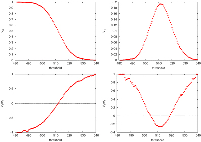
MFs versus density threshold of the realization of a Poissonian distribution of points.
The volume
 decreases monotonically as the threshold is increased and the high-density regions
  shrink.
The area
 first increases as the low-density regions
  expand and, after reaching a maximum, it decreases as the high-density regions
  shrink.
The average mean curvature
 increases monotonously from a negative value (
 is concave towards the shrinking high-density region) to a positive value (
 is convex towards the shrinking high-density region).
Finally, the genus
 is positive when
  looks bubble-like: there are many unconnected expanding low-density regions (‘holes’) at small
  , and many unconnected shrinking high-density regions (‘clusters’) at large
  is negative when
  is predominantly saddle-shaped: one observes many intertwined high- and low-density regions (‘tunnels’) at intermediate
  .
.
