


Abstract
We study the reionization history of the Universe in cosmological models with non-Gaussian density fluctuations, taking them to have a renormalized χ2 probability distribution function parametrized by the number of degrees of freedom, ν. We compute the ionization history using a simple semi-analytical model, considering various possibilities for the astrophysics of reionization. In all our models we require that reionization is completed prior to z= 6, as required by the measurement of the Gunn–Peterson optical depth from the spectra of high-redshift quasars. We confirm previous results demonstrating that such a non-Gaussian distribution leads to a slower reionization as compared to the Gaussian case. We further show that the recent WMAP three-year measurement of the optical depth due to electron scattering, τ= 0.09 ± 0.03, weakly constrains the allowed deviations from Gaussianity on the small scales relevant to reionization if a constant spectral index is assumed. We also confirm the need for a significant suppression of star formation in minihaloes, which increases dramatically as we decrease ν.
1 INTRODUCTION
The reionization of the Universe is a direct result of the formation of luminous sources which produce the photons responsible (see Barkana & Loeb 2001 for a review). Given that the first stars appear in low-mass haloes formed at high redshift, the reionization history of the Universe is expected to be a powerful probe of the amplitude and nature of density fluctuations on small scales.
The detection of Gunn–Peterson troughs (Gunn & Peterson 1965) in the absorption spectra of distant quasars suggests a late reionization for the Universe, at a redshift z∼ 6 (Becker et al. 2001; Fan et al. 2003; White et al. 2003; Fan et al. 2005; Gnedin & Fan 2006). The indications of a high optical depth from the first-year WMAP results (Kogut et al. 2003; Spergel et al. 2003), implying early reionization, led to a flurry of papers on quite complex ionization scenarios (e.g. Cen 2003; Chiu, Fan & Ostriker 2003; Ciardi, Ferrara & White 2003; Haiman & Holder 2003; Hui & Haiman 2003; Melchiorri et al. 2005). Simplicity has now largely been restored by the recent more precise third-year WMAP results (Page et al. 2006; Spergel et al. 2006), which indicate a much smaller optical depth, τ= 0.09 ± 0.03. This is consistent both with the quasar results and with a much simpler reionization history with a fast transition from a neutral to a ionized universe (see for example Choudhury & Ferrara 2006). Recent results by Haiman & Bryan (2006) suggest that this can only be achieved if star formation in high-redshift minihaloes has been significantly suppressed (see also Wyithe & Loeb 2006).
In this paper we perform a complementary study, investigating the dependence of the reionization history of the Universe on the nature of the cosmological perturbations, in the context of cosmologies permitted by the WMAP three-year results. We are motivated by the suggestions that a non-Gaussian contribution, for example from cosmic defects, might have been able to reconcile the high optical depth suggested by the WMAP first-year results and a low redshift of (complete) reionization implied by the quasar data (Chen et al. 2003; Avelino & Liddle 2004). With the new simpler ionization models, non-Gaussian models should be constrained better.
We compute the reionization history of the Universe using a simple semi-analytical model similar to that used by Haiman & Bryan (2006) (based on Haiman & Holder 2003). We consider various possibilities for the astrophysics of reionization, subject to the constraint that reionization is completed prior to z= 6 as required by the measurement of the Gunn–Peterson optical depth from the spectra of bright quasars at high redshift.
2 THE MASS FRACTION
We use the Press–Schechter approximation (Press & Schechter 1974) to compute the mass fraction, f(M), associated with collapsed objects with mass larger than a given mass threshold M. This was originally proposed in the context of initial Gaussian density perturbations, and later generalized to accommodate non-Gaussian initial conditions (Lucchin & Matarrese 1988; Chiu, Ostriker & Strauss 1998). In both cases the mass fraction is assumed to be proportional to the fraction of space in which the linear density contrast, smoothed on the scale M, exceeds a given threshold δc by
Here  is the one-point probability distribution function (PDF) of the linear density contrast δ, and Af is a constant which is computed by requiring that f(0) = 1 (Af= 2 in the case of Gaussian initial conditions). This generalization of the original Press–Schechter approximation has successfully reproduced the results obtained from N-body simulations with non-Gaussian initial conditions (Robinson & Baker 2000).
A top-hat filter will be used to perform the smoothing
where M= 4 πρmR3/3 (here ρm is the background matter density). We take δc= 1.7, motivated by the spherical collapse model and N-body simulations. For spherical collapse, δc is almost independent of the background cosmology (e.g. Eke, Cole & Frenk 1998).
The evolution of the dispersion of the density field is given by
where the suppression factor g(Ωm, ΩΛ) accounts for the dependence of the growth of density perturbations on the cosmological parameters Ωm and ΩΛ (Carroll, Press & Turner 1992; Avelino & de Carvalho 1999).
We will assume that the non-Gaussian density contrast has a χ2 PDF with ν degrees of freedom, the PDF having been shifted so that its mean is zero (such a PDF becomes Gaussian when ν→∞). Hence
where Q(a, x) with a > 0 is the incomplete gamma function defined by
Here
and Γ(a) =Γ(a, 0). When ν→∞ we have
3 THE POWER SPECTRUM
Historically, one of the main uncertainties in determining the reionization history of the Universe was the lack of an accurate determination of various cosmological parameters. However, these uncertainties have largely been removed by a growing body of precise cosmological data. Throughout, we will adopt a cosmological model motivated by the three-year WMAP results (Spergel et al. 2006). As they find that WMAP alone does not require a running of the spectral index, we will take as our base cosmology their preferred model with a power-law initial spectrum. The parameters are a matter density Ω0m= 0.24, dark energy density Ω0Λ= 0.76, baryon density Ω0B= 0.042, Hubble parameter h= 0.73, normalization σ8= 0.74 and perturbation spectral index n= 0.95.
To determine the amplitude of perturbations on the short scales relevant to reionization, we use the transfer function from Bardeen et al. (1986), so that the power spectrum is given by
where q=k/hΓ, [k]= Mpc−1,

and

is the shape parameter. The dispersion of the density field is given by
For Gaussian fluctuations, the Press–Schechter formalism leads to an underestimate of the halo mass function at the high-mass end (Jenkins et al. 2001), while the presence of baryons leads to a suppression of power on small cosmological scales. These two opposite effects are of the same order of magnitude and consequently we will ignore the baryon correction to the shape parameter (Sugiyama 1995). This is obviously a rather ad hoc procedure, but as no non-Gaussian equivalent of the Jenkins et al. mass function exists we have little choice. In the non-gaussian case, it has also been shown that small deviations from the predicted mass function could arise in particular in the limit of rare events (Avelino & Viana 2000; Inoue & Nagashima 2002). However, since we will fix the redshift at which reionization is to be completed by adjusting efficiency parameters, these uncertainties will not greatly affect our results.
4 THE REIONIZATION MODEL
Following Haiman & Bryan (2006) (see also Haiman & Holder 2003), we will classify dark matter haloes into three different categories according to their virial temperatures as following:
The total fraction of the mass in the Universe that is condensed into type II, Ia, and Ib haloes is given by


and
where the halo masses MII=MII(TII, z), MIa=MIa(TIa, z) and MIb=MIb(TIb, z) for the virial temperatures TII= 4 × 10² K, TIa= 104 K and TIb= 9 × 10⁴ K are obtained from
These haloes differ in their virial temperatures, and consequently in the cooling processes which are effective in each case. Ionizing sources can form in type II haloes only in the neutral regions of the intergalactic medium and provided there is a sufficient abundance of H2 molecules. On the other hand, type I haloes can cool and form ionizing sources independently of the H2 abundance. However, while type Ia haloes can form new ionizing sources only in neutral regions, the formation of new ionizing sources in type Ib haloes can also occur in the ionized regions of the intergalactic medium.
The recombination rate per unit of time and volume can be written as αBCH II〈nH II〉2, where αB is the recombination coefficient of neutral hydrogen to its excited states (= 2.6 × 10⁻¹³ cm3 s−1 at T= 104 K), 〈nH II〉 is the mean number density of ionized hydrogen and CH II≡〈n2H II〉/〈nH II〉2 is the mean clumping factor of ionized gas. Assuming that CH II does not vary with redshift, the probability P(ti, t) that a ionizing photon produced at a time ti is still contributing to reionization at a time t > ti is given by
where tr=αBCH IIXρB(ti) t2i/mp where ρB is the baryon density, X is the hydrogen mass fraction and mp is the proton mass. Alternatively, we may adopt the simple power-law relation of the evolution of the clumpiness CH II advocated by Haiman & Bryan (2006):
which in the β= 0 case reduces to CH II= 10.
The H ii filling factor FH II(z) is then obtained from the collapsed gas fractions as
where εI and εII are, respectively, the efficiencies (number of ionizing photons produced per proton in collapsed regions) of type I and type II haloes (it is being assumed that the efficiencies in type Ia and Ib are equal). The second term in the right-hand side of equation (18) includes a factor of (1 −FH II), which explicitly takes into account the fact that new ionizing sources should appear in type II and type Ia haloes only in regions which have not yet been ionized. The injection efficiency, ε, of ionizing photons into the intergalactic medium can be parametrized as ε=Nγf*fesc. Here f* is the fraction of baryons that turn into stars, Nγ is the average number of ionizing photons produced per stellar proton and fesc is the fraction of these ionizing photons which escape into the intergalactic medium.
Type II haloes are expected to host very massive stars, which are efficient at generating ionizing photons. On the other hand, it is expected that only a small fraction of the available gas will be incorporated into stars. Type I haloes are less efficient at producing ionizing photons, but that is compensated by a larger f*. In this paper, we will assume that the efficiencies do not depend on z and consider the values advocated by Haiman & Bryan (2006) for type II haloes, that is, Nγ= 80 000, f*= 0.0025 and fesc= 1, so that εII= 200 if no suppression of star formation in type II haloes occurs (εII= 0 otherwise). We fix the efficiency of type I haloes such that the Universe becomes fully ionized at z= 6.5. This means that εI depends on ν. However, we find that the efficiencies are lower only by a factor of approximately 2 in the ν= 1 case compared to the ν→∞ one. In the Gaussian case this approximately corresponds to the parameters chosen by Haiman & Bryan (2006), that is, Nγ∼ 4000, f*∼ 0.15 and fesc∼ 0.2 for type Ia and type Ib haloes so that εI∼ 120.
The optical depth is calculated using
where
The factor of 1.08 approximately accounts for the contribution of helium reionization. Here, we assume that H ii and He ii fractions are identical and that the He ii to He iii transition takes place at z < 6.
5 RESULTS
In Fig. 1 we plot the mass fraction in type II, type Ia and type Ib haloes, as a function of redshift z, for χ2 distributions with different numbers of degrees of freedom (ν= 1, 10, 100, ∞). We clearly see that the evolution of mass fraction with redshift becomes more gradual for smaller values of ν, thus making reionization a slower process in the non-Gaussian case. This can be confirmed in Fig. 2 where we plotted the evolution of the corresponding ionized fraction of hydrogen as a function of redshift z, for two possible ionization histories. In each case, we required that reionization is completed by z= 6.5. The solid line represents a reionization model with no contribution from type II haloes (εII= 0), while the dotted line represents a model where type II haloes are the dominant ionization source at high redshift (εII= 200). As expected, the slower evolution of the mass fraction in type Ia, type Ib and type II haloes with redshift at small ν is reflected in the evolution of ionized fraction of hydrogen, which also becomes a slower function of redshift.
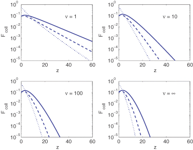
The evolution of the mass fraction, Fcoll, in type II, type Ia and type Ib haloes (solid, dashed and dotted lines, respectively), as a function of redshift z, for χ2 distributions with different numbers of degrees of freedom (ν= 1, 10, 100, ∞).
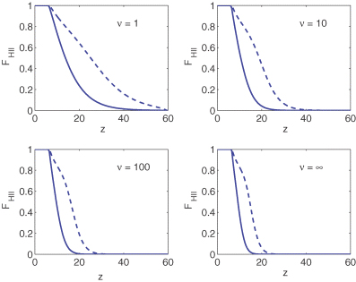
The evolution of the ionization fraction of hydrogen, FH II, as a function of redshift, z, for the mass fractions considered in Fig. 1 and for two possible ionization histories. εI is chosen so that reionization is completed by z= 6.5. The solid and dotted lines represent reionization models with εII= 0 (negligible contribution from type II haloes) and εII= 200 (type II haloes are the main ionization source at high redshift), respectively. Here, we assumed that the clumping factor, CH II, is given by equation (17) with β= 2.
Table 1 shows the accumulated optical depth to high redshift due to Thomson scattering, for the models shown in Fig. 2. Here, we confirm the results of Haiman & Bryan (2006) showing that in order not to overproduce the optical depth, star formation in minihaloes appears to have been suppressed even if we assume Gaussian fluctuations. As we decrease ν the need for this suppression increases dramatically.
The integrated optical depth (up to z= 60) due to Thomson scattering for the models considered in Fig. 2.
| ν | εII | τ |
|---|---|---|
| 1 | 0 | 0.17 |
| 1 | 200 | 0.36 |
| 10 | 0 | 0.10 |
| 10 | 200 | 0.21 |
| 100 | 0 | 0.09 |
| 100 | 200 | 0.16 |
| ∞ | 0 | 0.08 |
| ∞ | 200 | 0.14 |
| ν | εII | τ |
|---|---|---|
| 1 | 0 | 0.17 |
| 1 | 200 | 0.36 |
| 10 | 0 | 0.10 |
| 10 | 200 | 0.21 |
| 100 | 0 | 0.09 |
| 100 | 200 | 0.16 |
| ∞ | 0 | 0.08 |
| ∞ | 200 | 0.14 |
In Fig. 3, we show the impact of two different parametrizations for the evolution of the clumping factor (β= 2 and 0) on the reionization history of the Universe. We see that the poor knowledge of the redshift dependence of the clumping factor, CH II(z), introduces significant uncertainties in the predicted reionization history, which become increasingly large at small ν.
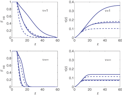
The evolution of the ionization fraction of hydrogen, FH II, and the integrated optical depth due to Thomson scattering, τ, as a function of redshift, z, for a model with ν= 1 (top panel) and a model with ν=∞ (bottom panel). Here, we consider two possible ionization histories with εII= 0 (negligible contribution from type II haloes) and εII= 200 (type II haloes are the main ionization source at high redshift) and two different evolutions for the clumping factor parametrized by β= 2 (solid line) and β= 0 (dashed line).
Finally, in Fig. 4 we plot the integrated optical depth (up to z= 60) due to Thomson scattering, τ, as a function of the number of χ2 degrees of freedom considering different evolutions for the clumping factor parametrized by β= 2 (solid line), β= 1 (dashed line) and β= 0 (dotted line) and a reionization model with a negligible contribution from type II haloes (εII= 0). The horizontal stripe represents the range of τ allowed by the WMAP three-year data (at 68 per cent confidence level). We see that given the model uncertainties reionization alone cannot yet rule out any value of ν with a significant degree of confidence.
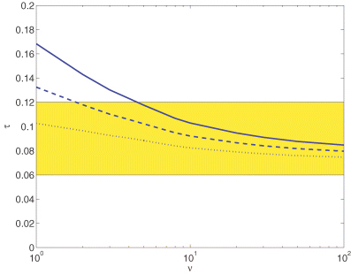
The integrated optical depth (up to z= 60) due to Thomson scattering, τ, as a function of the number of χ2 degrees of freedom considering different evolutions for the clumping factor parametrized by β= 2 (solid line), β= 1 (dashed line) and β= 0 (dotted line) and a reionization model with εII= 0. The horizontal stripe represents the range of τ allowed by the WMAP three-year data (at 68 per cent confidence level).
Note that since the efficiencies of type I haloes are fixed in order that reionization is completed at z= 6.5, the statistical uncertainties in the WMAP three-year cosmological parameter estimates have a small impact on our results. If we allow the cosmological parameters to vary over the range allowed by WMAP, the corresponding change in the integrated optical depth (up to z= 60) in Fig. 4 is always less than 10 percent, with the main source of uncertainty coming from the error in σ8. This is significantly smaller than the 1σ uncertainty in the value of τ determined from the WMAP three-year data, and it is also much smaller than the uncertainty due to the poor knowledge of the redshift evolution of the clumping factor.
6 CONCLUSIONS
We have investigated the possible impact of non-Gaussian density perturbations on the reionization history of the Universe in the context of cosmological models with non-Gaussian density fluctuations with a renormalized χ2 PDF parametrized by the number of degrees of freedom, ν. We have focused on this choice of non-Gaussianity as it forms a well-defined series, highly non-Gaussian for small ν, which tends towards Gaussianity for large ν. These models have enhanced high-density peaks as compared to Gaussian perturbations. This is typical of non-Gaussian models in the literature, for instance inflation models where the linear term is subdominant to the quadratic one, or perturbations from defect models. We assumed a constant spectral index so that the amplitude of the density perturbations on the small scales relevant to reionization could be calibrated using the three-year WMAP results. We have confirmed the results of Haiman & Bryan (2006) suggesting a significant suppression of star formation in minihaloes. However, we note that if we had chosen a left-skewed probability distribution where the non-Gaussianity has the opposite effect (such as an inverted χ2), we would instead have a suppression of the number of high-density peaks, potentially alleviating the need for the suppression of minihalo star formation.
We have also shown that the reionization history of the Universe is able to constrain the non-Gaussian nature of the density perturbations. However, we have seen that reionization alone is not yet able to rule out any value of ν (although very small values of ν appear to be disfavoured). Given that large deviations from a Gaussian PDF on large cosmological scales are already excluded by the WMAP data, we conclude that unless the PDF has a strong scale dependence, the cosmic reionization constraints are not competitive with those coming from the cosmic microwave background anisotropies. Still, it is important to bear in mind that the scales probed by reionization are much smaller than those probed by the WMAP (or even Planck), and consequently the consistency is reassuring, in particular taking into account recent claims (Mathis, Diego & Silk 2004) of hints for non-Gaussianity on scales much larger than those relevant for reionization.
We should also emphasize that our assumption of a constant spectral index excludes an important class of models, where the density field is the sum of Gaussian and non-Gaussian contributions with different power spectra. On large cosmological scales, the non-Gaussian component is severely constrained and only very small deviations from Gaussianity are allowed. However, if the power spectrum of the Gaussian contribution is steeper than that of the non-Gaussian one, as happens in hybrid models with both inflationary and defect perturbations, the non-Gaussian part may be the dominant component on small scales while being completely negligible on large cosmological scales.
Avelino & Liddle (2004) have recently shown that the reionization history of the Universe leads to stringent constraints on the energy scale of defects (see also Olum & Vilenkin 2006). However, since in that case the redshift at which the Universe becomes fully ionized no longer fixes the efficiencies of type I haloes, the analysis is more dependent on the astrophysics of reionization. We will return to this issue in a forthcoming publication.
PPA was supported by Fundação para a Ciência e a Tecnologia (Portugal) under contract POCTI/FP/FNU/50161/2003, and ARL by PPARC (UK). ARL thanks Jerry Ostriker for a useful discussion.
