


Abstract
Jets of gas released from young stars excavate cavities and drive bipolar outflows. The outflow properties may be related to the speed of the jets. To test this, we study the propagation of supersonic overdense jets through axisymmetric hydrodynamic simulations with radiative cooling and chemistry, building on previous studies by injecting molecular and atomic jets with a wide range of speeds, between 50 and 300 km s−1, into both molecular and atomic media. We show that the high collimation of outflows driven by molecular jets holds for all jet speeds. At the higher speeds, we find that the jet Mach number is the critical parameter which determines the shape of the cavity and the cavity is filled with atomic gas. However, at low speeds the jet material is the key factor with atomic jets producing much wider cavities, whereas molecular jets produce narrow cool molecular sheaths. A Mach disc is associated with the leading edge of the atomic simulations, whereas oblique shocks which refocus the jet are found in molecular flows. We also examine the mass spectra (distribution of mass with radial velocity), generally finding quite shallow relationships for all jet speeds (i.e the γ index is typically 1–2). Steep molecular mass spectra are, however, associated with the atomic-jet–molecular-medium combination. We conclude that the properties of bipolar outflows possess signatures related to the jet speed but are probably more sensitive to other factors.
1 INTRODUCTION
Jets penetrate through obscuring gas cores to be detected in the extended environments of protostars (Reipurth & Bally 2001). Although continuous jets are rarely uncovered, infrared and optical observations have revealed distinct chains of knots and aligned bow shocks which suggest that they are more or less continuously supplied by collimated supersonic jets (Stanke, McCaughrean & Zinnecker 2002; Khanzadyan et al. 2004; McGroarty, Ray & Bally 2004). These jets are of high thrust and so are capable of evacuating cavities by sweeping-up and deflecting the ambient medium. They may thus be held responsible for forming bipolar nebulae and bipolar outflows (Bachiller 1996). The bipolar outflows are collimated to various degrees and often extend to parsecs from the launching protostar (Richer et al. 2000; McGroarty et al. 2004).
One specific problem emphasized recently is that the rate of flow of jet momentum may not be sufficient to supply the bipolar outflows (Su, Zhang & Lim 2004). This may be related to basic questions concerning the content of the jets, their launch mechanism and the properties which allow them to propagate so far. To help find answers, numerical simulations have been executed which probe the relationship between the most probable jet properties and the observed outflow properties. To study the penetration, we assume that a supersonic jet has already been established but has not yet entered the extended envelope (e.g. Smith 2003). In this particular work, we present simulations which include radiative cooling and chemistry and examine the influence of the initial jet speed and molecular fraction.
Previous investigations of relevance have included a combination of radiative cooling, chemistry and magnetic field. Those restricted to atomic cooling processes include the investigations by Blondin et al. (1990), Stone & Norman (1993, 1994), Biro & Raga (1994), Frank et al. (1998), Cerqueira & de Gouveia dal Pino (1999), Gardiner et al. (2000), Stone & Hardee (2000) and Lee et al. (2001). On the other hand, powerful molecular jets occur in the earliest protostellar (and protoplanetary nebula) stages. Simulations which include molecular and atomic cooling, as well as some chemistry, are the simulations of Raga et al. (1995), Suttner et al. (1997), Downes & Ray (1999), Völker et al. (1999), O'Sullivan & Ray (2000), Downes & Cabrit (2003), Rosen & Smith (2003, 2004a) and Smith & Rosen (2005). In general, the simulations have provided reasonable interpretations for many of the observed outflows, as well as considerable insight into their dynamics and global evolution.
Each of these studies, however, considered a single nominal jet speed albeit with various pulsation and precession criteria. The chosen speed has ranged between 100 (e.g. O'Sullivan & Ray 2000) and 332 km s−1 (e.g. Stone & Hardee 2000). The question that remains to be answered is whether or not we can constrain the jet speed from the outflow structure. This is critical to answer since we might expect that the jet speed systematically increases with time, in proportion to the escape speed as a protostar builds up at, perhaps, constant density. On the other hand, the jet gas may switch from molecular to atomic as the mass available through accretion falls (e.g. Smith 2000). Therefore, we present here 11 simulations to cover these possibilities and so provide a basis from which to extract the signatures as jets gradually evolve from low speed to high speed and molecular to atomic (Section 3). For a quantitative comparison, we present the mass spectra (the mass as a function of radial velocity) in Section 4.
The simulations presented here are performed on a two-dimensional axisymmetric grid with a jet (hydrogen nucleon) density of 103 cm−3 (see Table 1). With these assumptions, we are able to reach a much higher resolution of the radiative layers behind shock waves than that achieved in previous works which were in three dimensions with typical jet densities of 105 cm−3 (Rosen & Smith 2003). The magnetic field has been omitted here but will be included in a subsequent work.
Summary of parameters in the atomic versus molecular runs.
| Property | Atomic | Molecular |
|---|---|---|
| Density, damb (gm cm−3) | 2.342 × 10⁻²² | 2.342 × 10⁻²² |
| Specific energy, eamb (erg K−1) | 2.278 × 10⁻¹² | 1.933 × 10⁻¹³ |
| n(H 2)/n | 1.000 × 10⁻⁵ | 5.000 × 10⁻¹ |
| Specific heat ratio, γ | 1.6667 | 1.4286 |
| Temperature, Tamb (K) | 100 | 10 |
| Temperature, Tjet (K) | 1000 | 100 |
| Mach number, Mjet: | ||
| 50 km s−1 | 15.21 | 70.33 |
| 100 km s−1 | 30.42 | 140.67 |
| 200 km s−1 | 60.83 | 281.34 |
| 300 km s−1 | 91.25 | 422.00 |
2 METHOD
zeus-3d is a computational fluid dynamics code for astrophysical flows (Stone & Norman 1992). We use a modified version which incorporates a module for molecular and atomic cooling. These routines use a semi-implicit method for calculating molecular and atomic hydrogen fractions along with the temperature, and were adopted from a version written by Suttner et al. (1997). The routines have been improved to include a limited equilibrium C and O chemistry, in order to calculate the CO, OH and H2 abundances. Details and tests were presented in the appendices of Smith & Rosen (2003).
We checked our revised code against the adiabatic and atomic simulations presented by Stone & Hardee (2000), finding general agreement of the global flow pattern, although individual features vary in the highly turbulent flow in and around the jet head (note that our cooling functions are more complete at lower temperatures). We set our initial and boundary conditions similar to those of Stone & Hardee (2000). Further fine-scale structure appears in our simulations due to the higher resolution. Stone & Hardee (2000) ran two-dimensional axisymmetric simulations on a grid of 2000 × 400 zones, whereas we take 4000 × 800 zones, maintaining the same initial jet radius, Rj= 2.5 × 1015 cm and overall spatial dimensions.
Hence, there are 20 zones per jet radius, 20 jet radii in radial direction and 100 jet radii in the axial direction. Therefore, the actual extent of the grid is (2.5 × 1017 cm) × (5 × 1016 cm).
We model a heavy (i.e. ballistic) jet in all cases. The ambient medium density is set to 100 cm−3 and the jet density is set to 1000 cm−3; hence, the introduced jet is overdense with respect to the ambient medium by the factor η= ρj/ρa= 10.
In our molecular simulations, the molecular hydrogen abundance in both the jet and the ambient medium is set to 0.5 (fully molecular). The abundances of free carbon and oxygen are both set to 10−4. The temperature of the ambient medium is set to 10 K and that of the jet is set to 100 K. In all cases, the jet is overpressured with respect to the ambient medium by the factor κ= Pj/Pa= 100.
In our atomic simulations, we retain all the cooling functions activated but greatly reduce the densities of molecular species. The molecular hydrogen fraction is now 10−5 and our abundances of carbon and oxygen are 10−6. This ensures that the atomic radiative cooling approximation controls the cooling.
The four jet velocities chosen are as listed below.
- (i)
A very slow jet, 50 km s−1;
- (ii)
a slow jet, 100 km s−1;
- (iii)
an intermediate jet, 200 km s−1; and
- (iv)
and a fast jet, 300 km s−1.
The actual input parameter which zeus converts into a jet speed is the Mach number (Mjet=Vjet/cjet). It depends on the sound speed in the jet, cjet, which is significantly higher in the atomic jet (3.29 km s−1) than in the molecular jet (0.711 km s−1).
3 RESULTS
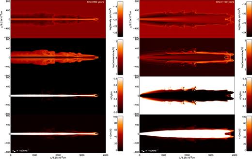
Figs 1–4 contain visualizations of the eight basic simulations. For each of the four speeds, the atomic jet-cloud results are displayed on the left-hand panels and the molecular jet-cloud results on the right-hand panels. Each plot consists of four panels with a grey-scale (colour in the electronic version) gradient scaling. We will use the following naming convention, in order to label the runs: 50A, 100A, 200A and 300A for the 50, 100, 200 and 300 km s−1 atomic runs, respectively, and 50M, 100M, 200M and 300M for the equivalent molecular runs.
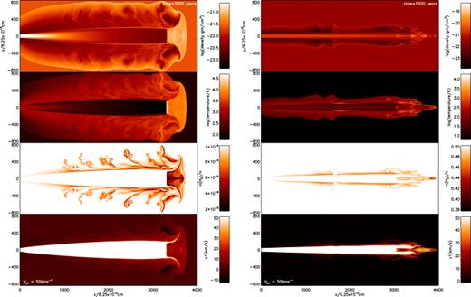
Cross-sectional distributions of physical parameters generated by jets of speed 50 km s−1. Left-hand panels: simulation of an atomic jet into an atomic medium (50A); right-hand panels: simulation of a molecular jet into a molecular medium (50M). As labelled, the parameters shown are the mass density (gm cm−3), temperature, molecular fraction and axial speed from top to bottom panel. The lower half of each distribution is the mirror image of the top half. Note the large lateral spreading of the cavity in the atomic case.
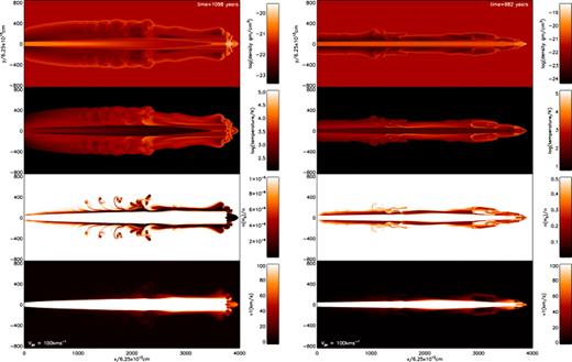
Cross-sectional distributions of physical parameters generated by jets of speed 100 km s−1. Left-hand panels: simulation of an atomic jet into an atomic medium (100A); right-hand panels: simulation of a molecular jet into a molecular medium (100M). As labelled, the parameters shown are the mass density, temperature, molecular fraction and axial speed from the upper to lower panel.
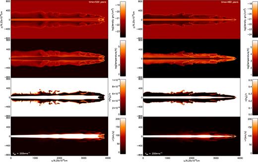
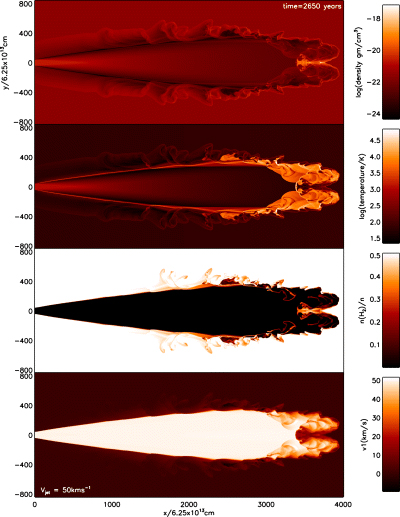
Cross-sectional distributions of physical parameters generated by jets of speed 200 km s−1. Left-hand panels: simulation of an atomic jet into an atomic medium (200A); right-hand panels: simulation of a molecular jet into a molecular medium (200M). As labelled, the parameters shown are the mass density, temperature, molecular fraction and axial speed from top to bottom panel.
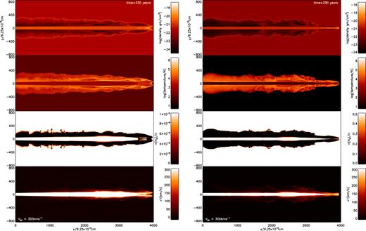
Cross-sectional distributions of physical parameters generated by jets of speed 300 km s−1. Left-hand panels: simulation of an atomic jet into an atomic medium (300A); right-hand panels: simulation of a molecular jet into a molecular medium (300M). As labelled, the parameters shown are the mass density, temperature, molecular fraction and axial speed from the upper to lower panel.
An additional molecular jet–atomic ambient medium run will be labelled as MJAA (Fig. 5, left-hand panels) and two additional atomic jet–molecular ambient medium runs will be labelled as AJMA for a 100 km s−1 jet (Fig. 5, right-hand panels) and AJMA50 for a 50 km s−1 jet (Fig. 6).
Cross-sectional distributions of physical parameters generated by jets of speed 100 km s−1 and with contrasting composition of the jet and ambient medium. Left-hand panels: simulation of a molecular jet into an atomic medium (MJAA); right-hand panels: simulation of an atomic jet into a molecular medium (AJMA). As labelled, the parameters shown are the mass density, temperature, molecular fraction and axial speed from the upper to lower panel.
Cross-sectional distributions of physical parameters generated by an atomic jet of speed 50 km s−1 propagating into a molecular medium (AJMA50), for comparison to Fig. 5, right-hand panels. As labelled, the parameters shown are the mass density, temperature, molecular fraction and axial speed from the upper to lower panel.
The panels display the following information.
- 1
The upper panels display the mass density plotted on a logarithmic scale. Also shown is the time in years corresponding to the displayed distributions, just before each jet has reached the end of the grid.
- 2
The second panels display the temperature, again on a logarithmic scale.
- 3
The third panels trace the molecular fraction or, more precisely, the ratio of hydrogen molecules to the total number of hydrogen nuclei [n(H 2)/n]. Note that the distribution of molecular fraction in both the atomic and molecular runs appears similar at first glance. Molecular cooling does actually take place in the atomic cases, but the quantities of molecular material are many times smaller. As seen from the scale bars, the molecular density is 100 000 times less in the atomic cases.
- 4
The lower panels display the axial component of velocity in km s−1. This clearly shows the expansion and extent of the jet beam.
The most dramatic contrast between the atomic and molecular runs occurs at the lowest speed of 50 km s−1 (Fig. 1). Here, the relatively low Mach number of the atomic jet is responsible for a high transverse jet expansion. This leads to the blow-torch structure at the jet inlet and the high density gradient along the jet axis (upper panel). The result is that the leading edge of the outflow decelerates with an average speed of advance of ∼26.4 km s−1.
The termination shock of the atomic jet takes the form of a large Mach disc which generates warm atomic gas. This gas is slow to cool for the chosen density, thus (i) supporting the Mach disc, and (ii) forming the wide low-density cavity of temperature 3000–8000 K (second panel). However, at considerably higher densities, further cooling mainly through gas–grain collisions will cool the gas down to ∼1000 K on a time-scale of 108/n yr (Smith & Rosen 2003), reducing the cavity size. The cavity also contains wisps of hot shocked gas within which small quantities of residual molecules are also destroyed (third panel). The displayed axial velocity illustrates the low advance speed of ∼20 km s−1, as well as a back-flow (negative v1, see scale bar to the fourth panel) typical of underdense jets.
On the other hand, the low-speed molecular jet (with Mach number of 70) displays only moderate expansion (lower panel). As a consequence, the advance of the leading edge is maintained with an average speed of ∼38.6 km s−1. However, the region where the jet terminates is complex. A nose develops where the jet material becomes focused towards the axis [such structure is also present in three-dimensional Cartesian simulations of molecular jets (Rosen & Smith 2003)]. The strong molecular cooling does not allow a Mach disc to develop but leads, instead, to oblique shocks. The cavity is also narrow because of the maintained collimation and the high advance speed. Therefore, unlike the atomic case, no back-flow in the cavity arises (lower panel).
At 100 km s−1 (Fig. 2), the low-speed features are still apparent in a diluted form. The atomic simulation generates a cavity of roughly half the size of the lower-speed case. The Mach disc is fragmentary and no back-flow occurs. The cavity in the molecular simulation is more pointed in shape. A prominent ‘shoulder’ occurs causing jet expansion followed by focusing. This results in a remarkable vortex-like structure in the cavity, as prominent in the molecular fraction panel. An oblique shock is present between the vortex and the jet (see top and second panels of Fig. 2) which results in the jet focusing.
At 200 km s−1 (Fig. 3), expansion of the atomic jet is not prominent and the average advance speed of the atomic jet is only 10 per cent higher than that of the molecular jet. Both cavities are narrow and the cavities now almost exclusively contain atomic gas in both cases. The main difference is that the refocusing shoulders remain in the molecular jet, whereas the leading edge of the atomic jet is a blunt structure, inflated by warm shocked atomic gas.
At 300 km s−1 (Fig. 4), the collimation is slightly improved in both cases. High-speed atomic jets also display a hotter sheath to the jet. Although small-scale structures near the jet heads differ, the global outflow structures are quite similar.
We ran three additional simulations: one of a molecular jet propagating into an atomic medium at 100 km s−1 (MJAA, Fig. 5, left-hand panels), and two of an atomic jet propagating into a molecular medium at 100 (AJMA, Fig. 5, right-hand panels) and 50 km s−1 (AJMA50, Fig. 6). The standard parameters from Table 1 were used and they can be most closely compared to the other 100 km s−1 jets in Fig. 2 and to the 50A jet in Fig. 1, left-hand panels. Of these additional simulations, AJMA and AJMA50 contain the most significant difference from the 100A and 50A runs, atomic jets moving through atomic media. Although the jet has expanded, the cavity is very narrow. The Mach disc is replaced by oblique shocks as ambient molecular material gets trapped near the jet axis. The MJAA simulation has a narrower jet beam than that of the 100M run. The hotter cavity is responsible for confining a more uniform jet. The cavity itself is slightly wider and conical.
To summarize, atomic jets are terminated either by a Mach disc or by deflection away from the jet axis. Molecular jets tend to be focused towards the axis, by oblique shocks, producing shouldered structures and narrow advancing noses. Much of the global structure is related to the Mach number of the jet flow which determines the transverse expansion, until the cavity pressure can provide resistance. Thus, high Mach number jets generate narrow cavities. Note the similarity in the global structure of 200A and 50M, including the width of the jets where the terminal Mach discs occur. This results from the similar jet Mach numbers of these two simulations. At jet speeds in excess of 100 km s−1, the entire cavity is filled with atomic gas. Below this value, the cavity can be occupied by both molecular and atomic materials.
4 DISTRIBUTION OF MASS WITH VELOCITY
4.1 Mass–velocity relationships
To aid the exploration of how momentum is transferred from the jet to the ambient medium, a function of the form dm/dv∝v−γ is fitted to the data of protostellar outflows. Here, m is the spatially integrated mass as a function of radial velocity, v, referred to as the mass spectrum. The mass is usually derived from the intensity of the radiation from optically thin spectral lines associated with low-rotational CO transitions (e.g. Yu et al. 2000).
The value of γ depends on the velocity range being approximated. Some observational surveys have shown broken power laws (Yu et al. 2000; Su et al. 2004). This usually consists of a shallow slope, 1.0–2.0, at low velocities connecting to a steeper slope, and as large as 10, at higher velocities (Ridge & Moore 2001). The velocity of the breakpoint is typically ∼10 km s−1.
A break in the mass spectra, referred to as a dip, was indeed found in three-dimensional simulations by Smith, Suttner & Yorke (1997), and was caused by the ineffective survival of molecules over the leading bow shock. Note that there are several uncertain factors, such as the optical depth, dependence of opacity on velocity, subtraction of mass associated with the ambient cloud, orientation of the flow, confusion from other outflows and time-variable mass loss.
To date, simulations have had difficulty matching the entire range of observed mass spectra. Simulations of molecular jets (both ballistic and non-ballistic) have given fairly low γ values such as 1.2–1.6 (Smith et al. 1997), ∼1.5 (Downes & Cabrit 2003) and even shallower (0.9–1.3) (Rosen & Smith 2004b). Arce & Goodman (2001) suggested that a steeper mass–velocity slope can be obtained if the outflow has an episodic nature. Smith et al. (1997) and Downes & Ray (1999) suggested that γ increases with time as ambient material which has been entrained slows down leading to more mass at lower velocities. Most recently, Keegan & Downes (2005) investigated the mass–velocity and intensity–velocity relations in simulations of long-duration jet-driven molecular outflows up to 2300 yr. They found that γ increases to ∼1.6 until t∼ 1500 yr, after which point it remains fairly constant.
Rosen & Smith (2004a) found that the values of γ of atomic driven outflows are small at low radial velocities, and steepen slightly at larger viewing angles and for larger radial velocities (the viewing angle defined here is the angle between the jet and the plane of the sky). The mass with velocities less than the break velocity are associated with ambient material entrained by the bow shock wings, whereas velocities greater than the break velocity are related to entrainment adjacent to the bow shock head. Furthermore, both at very low viewing angles and at large viewing angles, the slope in the highest radial velocity range can be as high as 10.
4.2 Dependence on jet speed
In order to derive the mass spectra, we revised a three-dimensional routine to read in the axisymmetric data (taking into account symmetries for computational efficiency). The cylinder is divided into segments in the radial direction, r, and a series of divisions along the jet axis. The projected velocity of each segment at the chosen viewing angle, α, out of the plane of the sky is then calculated and the mass placed into a series of radial velocity bins.
One ancillary consequence of this method is that the material in the jet beam itself is included, forming a sharp peak at the highest |Vrad| extent at vjet sin α.
We calculated mass spectra for the atomic and molecular runs at the four jet speeds for five viewing angles of α: 15°, 30°, 45°, 60° and 90°. We applied the IDL linfit algorithm to calculate the resultant mass–velocity power-law slopes across four fixed radial velocity ranges: 2–4, 4–8, 8–16 and 16–32 km s−1, hereafter referred to as velocity intervals ‘A’, ‘B’, ‘C’ and ‘D’, respectively. This leads to objective values of γ which can be compared directly with other runs and viewing angles. Table 2 contains the γ values for the runs at all the viewing angles and we display the mass spectra for the 45° viewing angle in Fig. 7.
The estimated ‘γ’ values for the molecular and atomic runs at a viewing angle of 45° out of the plane of the sky. ‘A’ represents the range 2–4 km s−1, ‘B’ represents the range 4–8 km s−1, ‘C’ represents the range 8–16 km s−1 and ‘D’ represents the range 16–32 km s−1. The ‘ ’ entries replace non-sensical results where the local conditions caused a poor line fit.
| Angle | γ: | A | B | C | D | A | B | C | D | ||
|---|---|---|---|---|---|---|---|---|---|---|---|
| Run | Run | ||||||||||
| 15° | 50A | 1.527 | 4.318 |  | 3.647 | 50M | 0.781 | 0.585 | 2.978 |  | |
| 100A | 1.423 | 3.176 | 0.551 |  | 100M | 2.062 | 0.826 | 1.416 |  | ||
| 200A | 0.611 | 2.001 | 1.649 |  | 200M | 1.516 | 1.083 | 1.804 | 1.292 | ||
| 300A | 0.148 | 1.270 | 3.309 | 0.718 | 300M |  | 2.079 | 1.481 | 2.085 | ||
| 30° | 50A | 1.800 | 1.432 | 4.936 |  | 50M | 1.138 | 0.595 | 0.226 |  | |
| 100A | 1.440 | 2.676 | 0.573 | 0.701 | 100M | 1.907 | 1.988 | 0.134 | 0.986 | ||
| 200A | 0.982 | 1.928 | 1.563 | 1.511 | 200M | 1.894 | 1.372 | 1.379 | 1.395 | ||
| 300A | 0.174 | 1.478 | 3.230 | 1.597 | 300M |  | 2.170 | 1.346 | 1.739 | ||
| 45° | 50A | 2.61 | 0.191 | 6.84 |  | 50M | 1.116 | 0.588 | 0.164 |  | |
| 100A | 1.51 | 1.97 | 1.04 | 0.541 | 100M | 1.418 | 1.317 | 0.539 | 1.046 | ||
| 200A | 1.39 | 2.02 | 1.39 | 1.42 | 200M | 1.761 | 1.617 | 1.070 | 1.054 | ||
| 300A | 0.344 | 2.03 | 3.16 | 1.00 | 300M |  | 1.932 | 1.675 | 1.915 | ||
| 60° | 50A | 1.634 | 1.169 |  | 2.290 | 50M | 1.138 | 0.703 | 0.973 | 0.259 | |
| 100A | 2.102 | 1.452 | 0.870 | 0.537 | 100M | 1.516 | 1.328 | 1.146 | 0.282 | ||
| 200A | 1.163 | 2.239 | 1.083 | 1.405 | 200M | 0.922 | 1.280 | 1.370 | 1.830 | ||
| 300A | 0.734 | 2.290 | 2.371 | 0.919 | 300M | 0.952 | 1.264 | 1.607 | 1.437 | ||
| 90° | 50A | 0.0957 | 2.325 | 2.071 | 3.641 | 50M | 1.351 | 0.713 | 0.758 |  | |
| 100A | 1.309 | 2.218 | 0.573 | 1.573 | 100M | 1.977 | 0.891 | 0.836 | 0.473 | ||
| 200A | 0.962 | 2.033 | 0.892 | 1.564 | 200M | 0.597 | 0.689 | 1.553 | 1.425 | ||
| 300A | 1.556 | 1.688 | 2.066 | 1.020 | 300M | 0.993 | 1.054 | 1.058 | 1.593 | ||
| Angle | γ: | A | B | C | D | A | B | C | D | ||
|---|---|---|---|---|---|---|---|---|---|---|---|
| Run | Run | ||||||||||
| 15° | 50A | 1.527 | 4.318 | | 3.647 | 50M | 0.781 | 0.585 | 2.978 | | |
| 100A | 1.423 | 3.176 | 0.551 | | 100M | 2.062 | 0.826 | 1.416 | | ||
| 200A | 0.611 | 2.001 | 1.649 | | 200M | 1.516 | 1.083 | 1.804 | 1.292 | ||
| 300A | 0.148 | 1.270 | 3.309 | 0.718 | 300M | | 2.079 | 1.481 | 2.085 | ||
| 30° | 50A | 1.800 | 1.432 | 4.936 | | 50M | 1.138 | 0.595 | 0.226 | | |
| 100A | 1.440 | 2.676 | 0.573 | 0.701 | 100M | 1.907 | 1.988 | 0.134 | 0.986 | ||
| 200A | 0.982 | 1.928 | 1.563 | 1.511 | 200M | 1.894 | 1.372 | 1.379 | 1.395 | ||
| 300A | 0.174 | 1.478 | 3.230 | 1.597 | 300M | | 2.170 | 1.346 | 1.739 | ||
| 45° | 50A | 2.61 | 0.191 | 6.84 | | 50M | 1.116 | 0.588 | 0.164 | | |
| 100A | 1.51 | 1.97 | 1.04 | 0.541 | 100M | 1.418 | 1.317 | 0.539 | 1.046 | ||
| 200A | 1.39 | 2.02 | 1.39 | 1.42 | 200M | 1.761 | 1.617 | 1.070 | 1.054 | ||
| 300A | 0.344 | 2.03 | 3.16 | 1.00 | 300M | | 1.932 | 1.675 | 1.915 | ||
| 60° | 50A | 1.634 | 1.169 | | 2.290 | 50M | 1.138 | 0.703 | 0.973 | 0.259 | |
| 100A | 2.102 | 1.452 | 0.870 | 0.537 | 100M | 1.516 | 1.328 | 1.146 | 0.282 | ||
| 200A | 1.163 | 2.239 | 1.083 | 1.405 | 200M | 0.922 | 1.280 | 1.370 | 1.830 | ||
| 300A | 0.734 | 2.290 | 2.371 | 0.919 | 300M | 0.952 | 1.264 | 1.607 | 1.437 | ||
| 90° | 50A | 0.0957 | 2.325 | 2.071 | 3.641 | 50M | 1.351 | 0.713 | 0.758 | | |
| 100A | 1.309 | 2.218 | 0.573 | 1.573 | 100M | 1.977 | 0.891 | 0.836 | 0.473 | ||
| 200A | 0.962 | 2.033 | 0.892 | 1.564 | 200M | 0.597 | 0.689 | 1.553 | 1.425 | ||
| 300A | 1.556 | 1.688 | 2.066 | 1.020 | 300M | 0.993 | 1.054 | 1.058 | 1.593 | ||
The estimated ‘γ’ values for the molecular and atomic runs at a viewing angle of 45° out of the plane of the sky. ‘A’ represents the range 2–4 km s−1, ‘B’ represents the range 4–8 km s−1, ‘C’ represents the range 8–16 km s−1 and ‘D’ represents the range 16–32 km s−1. The ‘’ entries replace non-sensical results where the local conditions caused a poor line fit.
| Angle | γ: | A | B | C | D | A | B | C | D | ||
|---|---|---|---|---|---|---|---|---|---|---|---|
| Run | Run | ||||||||||
| 15° | 50A | 1.527 | 4.318 | | 3.647 | 50M | 0.781 | 0.585 | 2.978 | | |
| 100A | 1.423 | 3.176 | 0.551 | | 100M | 2.062 | 0.826 | 1.416 | | ||
| 200A | 0.611 | 2.001 | 1.649 | | 200M | 1.516 | 1.083 | 1.804 | 1.292 | ||
| 300A | 0.148 | 1.270 | 3.309 | 0.718 | 300M | | 2.079 | 1.481 | 2.085 | ||
| 30° | 50A | 1.800 | 1.432 | 4.936 | | 50M | 1.138 | 0.595 | 0.226 | | |
| 100A | 1.440 | 2.676 | 0.573 | 0.701 | 100M | 1.907 | 1.988 | 0.134 | 0.986 | ||
| 200A | 0.982 | 1.928 | 1.563 | 1.511 | 200M | 1.894 | 1.372 | 1.379 | 1.395 | ||
| 300A | 0.174 | 1.478 | 3.230 | 1.597 | 300M | | 2.170 | 1.346 | 1.739 | ||
| 45° | 50A | 2.61 | 0.191 | 6.84 | | 50M | 1.116 | 0.588 | 0.164 | | |
| 100A | 1.51 | 1.97 | 1.04 | 0.541 | 100M | 1.418 | 1.317 | 0.539 | 1.046 | ||
| 200A | 1.39 | 2.02 | 1.39 | 1.42 | 200M | 1.761 | 1.617 | 1.070 | 1.054 | ||
| 300A | 0.344 | 2.03 | 3.16 | 1.00 | 300M | | 1.932 | 1.675 | 1.915 | ||
| 60° | 50A | 1.634 | 1.169 | | 2.290 | 50M | 1.138 | 0.703 | 0.973 | 0.259 | |
| 100A | 2.102 | 1.452 | 0.870 | 0.537 | 100M | 1.516 | 1.328 | 1.146 | 0.282 | ||
| 200A | 1.163 | 2.239 | 1.083 | 1.405 | 200M | 0.922 | 1.280 | 1.370 | 1.830 | ||
| 300A | 0.734 | 2.290 | 2.371 | 0.919 | 300M | 0.952 | 1.264 | 1.607 | 1.437 | ||
| 90° | 50A | 0.0957 | 2.325 | 2.071 | 3.641 | 50M | 1.351 | 0.713 | 0.758 | | |
| 100A | 1.309 | 2.218 | 0.573 | 1.573 | 100M | 1.977 | 0.891 | 0.836 | 0.473 | ||
| 200A | 0.962 | 2.033 | 0.892 | 1.564 | 200M | 0.597 | 0.689 | 1.553 | 1.425 | ||
| 300A | 1.556 | 1.688 | 2.066 | 1.020 | 300M | 0.993 | 1.054 | 1.058 | 1.593 | ||
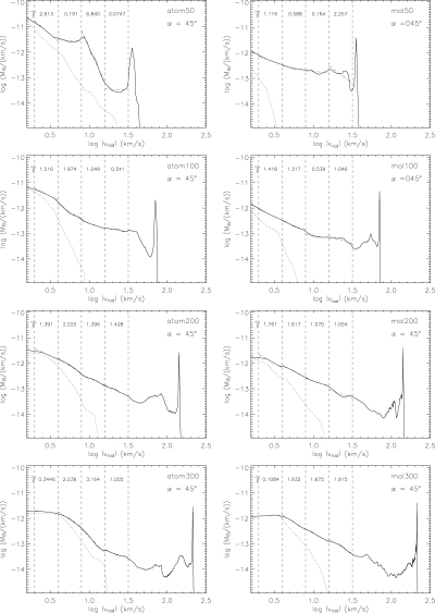
Mass spectra of the eight runs at a viewing angle of 45°. Both the redshifted and blueshifted emissions are displayed; the redshifted material being represented by the dotted lines. The vertical dashed lines mark the divisions of the velocity intervals mentioned in Table 2. A dot–dashed line is fitted to the mass–velocity spectrum within each velocity interval and the value of the slope of each line is printed near the top of each plot.
The power-law fits for the 16–32 km s−1 range (interval D) are not always useful as it is generally too fast at small viewing angles and low jet velocities. Intervals B and C provide consistent and comparable data. Note that the viewing angles of 15° and 90° do not hold completely systematic γ values, whereas the intermediate angles, 30°–60°, show systematic trends.
The mass spectra display expected features. The higher the jet velocity, the further the maximum |Vrad| extent. However, this does not imply that the mass spectrum becomes shallower. As shown in Fig. 7, the opposite is often the case within intervals B and C. This is probably due to the more aerodynamic shapes of the higher-speed flows which lead to proportionally less of the ambient medium being accelerated to high speeds. However, a moderately high γ value is not an indication of high speed, since various exceptions are recorded in Table 2.
Furthermore, the higher the viewing angle, the higher the maximum radial velocity. For example, the maximum point of 100M at 15° is 28 km s−1, whereas at 90° it is 100 km s−1, as would be expected from the jet radial component vjet sin α. We might thus expect the slope to become shallower. However, an inspection of the table reveals that it is true for 200A in velocity field C and 300A in velocity fields A and C, at 15° viewing angle, but not generally.
A further trend is that mass spectra of the atomic runs possess a convex shape (steepening towards higher radial speeds), whereas the molecular runs give a slight concave distortion within interval B. This may be related to the results of Rosen & Smith (2004a) who noted that for some of their simulations the power law may be better fitted with an exponential (1/e) curve.
The most pronounced shape is associated with run 50A which has a ‘speed hump’ at the true (deprojected) velocity of 12.6 km s−1. At 45° in Fig. 7 it produces a double-peaked mass spectrum. The most likely cause of this intermediate velocity spike is the extremely wide extended ‘working surface’ created by the 50A jet as seen in Fig. 1. In fact, all the atomic runs possess a larger working surface than that possessed by the molecular runs and this could be responsible for the slight convex shapes.
A detailed study of all the mass spectra demonstrates that the atomic outflows tend to produce larger values of γ than molecular outflows. This is particularly strong for the low-speed runs (Fig. 8, left-hand panel), whereas the mass spectra for high-speed runs roughly converge (see Fig. 8, right-hand panel). The mean value of all the slopes in the velocity interval B of the molecular runs is 1.2 and for the atomic runs it is 1.99. Repeating for velocity interval C gives 1.18 for the molecular runs and 2.12 for the atomic.
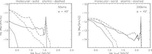
Mass spectra at 45° viewing angle out of the sky plane, depicting the molecular run with the heavy solid line and the atomic run with the heavy dashed line combined on the same plot for direct comparison purposes. Left-hand panel: 50km s−1 case. Right-hand panel: 200 km s−1 case. The lighter solid and dashed lines represent redshifted material.
Mass spectra for runs MJAA and AJMA are displayed in Fig. 9. They indicate that it is the ambient medium which mainly determines the value of γ. Overplotting MJAA and AJMA also clearly shows that AJMA possesses a greater amount of overall mass in motion. The expanded jet and the blunter leading edge in the AJMA run lead to a considerably larger volume of accelerated gas.
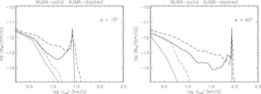
Superimposed mass spectra of the MJAA (solid line) and AJMA (dashed line) runs at the indicated orientations of the jet axis out of the sky plane. The lighter solid and dashed lines represent redshifted material.
To further complement the analysis, we created two additional mass–velocity plots of the AJMA and AJMA50 runs (Fig. 10). Here, we display the molecular mass rather than the total mass. As the jet beam is atomic, its contribution is reduced by a factor of 105. Furthermore, material impacting the leading bow shock is also dissociated. This effectively leaves only ambient material entrained through the wings of the advancing bow shock. In both cases shown, it leads to a significantly steeper molecular mass–velocity slope. A γ-value of ∼4 is reached in the 16–32 km s−1 interval. Fig. 10 also shows that the γ of the molecular mass is slightly larger than the γ of the total mass. A similar result was found in simulations by Downes & Cabrit (2003) and later by Rosen & Smith (2004a).
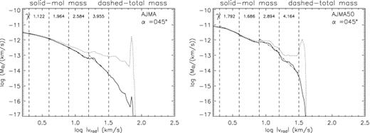
Molecular mass spectra at a 45° viewing angle out of the sky plane, for the two AJMA runs. The dotted line shows the original total mass result and the solid line signifies the molecular mass–velocity spectrum.
5 ANALYSIS AND DISCUSSION
5.1 Collimation
The most significant result is that molecular jets into molecular media generate highly collimated outflows at all jet speeds. This is due to a combination of two factors. First, the fact that the molecular jets have a lower sound speed, and therefore a higher Mach number than that of their atomic counterparts, implies that molecular jets display little transverse expansion. The Mach number of 100A is only 30, whereas for 100M it is 140 (see Table 1). Table 1 also highlights that a fundamental difference between the atomic and molecular runs is the temperature of the jet and the ambient medium. The choice of temperature would change the Mach number and hence the cavity shape.
Secondly, the molecular cooling through the leading edge and in the cavity reduces the extent of the cavity which remains inflated by a small fraction of warm atomic gas, corresponding to the dissociated fraction from the leading edge.
In the atomic cases, as the speed is raised the outflow structure becomes steadily more collimated. This is due to the differing grid crossing times coupled with the natural lateral expansion of the jet at the sound speed, cs. We would expect the longer the crossing time, the greater the lateral expansion. In 50A, the crossing time is over 2850 yr and the expansion is very notable compared to the 300A case which crosses the grid in a mere 330 yr. Lateral expansion times follow the Mach expansion rule of 1/Mjet. A visual estimation shows that at 3000 zones in the axial direction, the 50A jet has expanded 175 zones in the y-direction. This ratio is 17.1 which agrees with the Mach number of 15.21 from Table 1.
The molecular cooling jets do not exhibit a large lateral expansion despite similar crossing times. Although the 50M 2000 yr crossing time is faster than that of 50A, the cavity width retains fairly uniform collimation and is similar to that of the 300M jet. A similar calculation shows a 55-zone expansion after 3000 zones which suggests a Mach number of 55. The actual Mach number is in fact 70.
The runs with high molecular content reach greater densities than those achieved by the atomic runs. The molecules permit the compressed gas to cool, thus decreasing the pressure and so increasing the inward pressure gradient, causing the material to collapse. Our molecular cooling routines would allow the gas to cool as low as 1 K but the dust has a fixed temperature, set to 20 K, which quite effectively heats gas (by collisions) falling far below that temperature. On the other hand, cooling in the atomic runs is only significant above 200 K and is most effective for temperatures above 10 000 K. It should be noted that the simulations in this paper are of perfectly collimated jets with a 0° initial opening angle. If we were to take a non-zero opening angle in the form of a shear or a spray angle, it would lead to the creation of a complete range of cavity shapes independent of the initial Mach number and depending only on the initial opening angle.
5.2 Refocusing
An oblique internal shock is evident in the density plot of 100A which leads to the jet recollimation close to the front. Recollimation shoulders are evident to some degree in all the eight standard runs. These are small ‘kinks’ along the interface of the jet beam with the shocked ambient medium which hint at the presence of internal shocks within the jet cavity. In the molecular runs, the shoulders lead to a tight focusing of the jet beam towards the axis, whereas the ambient medium is deflected away from the axis by the oblique wings of a bow shock.
5.3 Molecular fraction
In the molecular cases, as the speed is raised, an increasing fraction of molecules are destroyed. In 50M, there is very little molecular destruction. The greatest dissociation occurs in a very small region at the head of the jet where it is most likely being compressed against the axis, but even at this point, the molecular fraction falls to only 0.38 (from 0.5).
The cavity of 100M is also mostly molecular, mainly between 0.2 and 0.5. At a region around 3000 zones in the axial direction, some ambient material appears to have just been entrained by a large vortex.
A transition occurs between 100 and 200 km s−1 as the 200M cavity is almost entirely atomic but with some hints of entrainment. An interesting feature, also at 3000 zones in the axial direction, is where ambient molecular material is being folded in and is now being dispersed.
The atomic runs show the molecular fraction changing in a way that appears similar to the molecular runs in that the molecular fraction decreases with velocity. However, the scaling of the atomic runs is in fact five orders of magnitude smaller. It is still interesting to note that such low fractions of molecular material also get destroyed. Note that at 200M and 300M there is still no significant reformation of molecules, given the density and time-scale (reformation requires roughly 1017/n s).
6 CONCLUSION
We have explored how outflow structure depends on the jet speed, building on our previous works which simulated protostellar outflows generated by 100 km s−1 molecular jets. We have assumed that the jet is initially highly collimated without precession in direction, pulsation or imposed spray angle. Each of these dynamical effects leads to distinct predictions.
We find that molecular jets into molecular media tend to produce highly collimated outflows because of their high Mach numbers. The transverse expansion of the jet at the sound speed depends on the initial jet temperature. The enveloping cavity is mainly filled with cool molecular gas for jet speeds at or under 100 km s−1 but is otherwise occupied by atomic gas.
The collimation is sensitive to the jet speed when atomic jets are launched into atomic media. The warm ballistic jets explored here are free to expand laterally which leads to wide cavities at low jet Mach numbers.
In all the molecular cases, the leading bow shock is acute with oblique shocks deflecting jet material towards the axis, whereas external shocks deflect the ambient gas off the axis. The result is that the high-pressure cavity gas remains adjacent to the jet, producing further oblique shocks which focus the jet gas towards the axis well before the leading edge. Extremely high rises in pressure occur at the working surfaces of high Mach number jets. In the molecular jets, the high pressure is maintained only within shock layers. The layers are maintained by ram pressure as the jet ploughs into ambient material. The aerodynamic shape results in two shock layers: a leading bow shock layer and a trailing highly oblique shock that provides jet focussing towards the axis.
On the other hand, in the atomic cases a transverse Mach disc is formed to terminate the low-speed jets. At speeds above 100 km s−1, the shock structure is more complex with jet deflection away from the axis.
This analysis suggests that we could tell whether a jet is atomic or molecular from its collimation only if the velocity is fairly low, <100 km s−1. High-velocity (∼300 km s−1) molecular jets could be confused with high-velocity atomic jets as the molecules get destroyed in the molecular jet, and the high speed of atomic jets effectively maintains the collimation.
For all the simulations presented here, we find similar (total) mass spectrum properties for the 100 km s−1 case, that is, quite shallow distributions. Therefore, higher jet speeds do not help to fully interpret observational statistics by producing steep mass spectra. In general, mass spectrum trends with jet velocity or orientation are very weak. At high speeds, there is little difference between atomic and molecular mass spectra. At low speeds, they are distinguishable with atomic jets producing significantly steeper mass spectra. However, atomic mass spectra are not directly observable with atomic line emission dominated by narrow ranges of physical conditions.
Molecular mass spectra may be directly related to the observed flux velocity CO profiles. Very rarely, however, has a prominent spike in CO profiles been observed which would be the signature of a molecular jet (Smith et al. 1997). Therefore, we presented here two examples of molecular outflows driven by atomic jets, finding not only that the jet velocity spike disappears, but also that the molecular mass spectrum steepens significantly above ∼6 km s−1.
Given these results, we conclude that other factors are required to provide the observed range of outflow properties. The magnetic field in the jet and density gradients in the ambient medium are two such factors we intend to examine. The present results provide the background for these studies.
This work benefitted through support from INTAS grant 03-51-4838.
