


Abstract
Standing, propagating or oscillating shock waves are common in accretion and winds around compact objects. We study the topology of all possible solutions using the pseudo-Kerr geometry. We present the parameter space spanned by the specific energy and angular momentum and compare it with that obtained from the full general relativity to show that the potential can work satisfactorily in fluid dynamics also, provided the polytropic index is suitably modified. We then divide the parameter space depending on the nature of the solution topology. We specifically study the nature of the standing Rankine–Hugoniot shocks. We also show that as the Kerr parameter is increased, the shock location generally moves closer to the black hole. In future, these solutions can be used as guidelines to test numerical simulations around compact objects.
1 INTRODUCTION
Since the black holes themselves do not emit radiations, identification of a black hole is to be carried out by the radiations emitted from the accretion flows and/or jets and outflows. Thus, it is imperative that the accretion matter be studied for all possible boundary conditions. Although the most well-accepted theory of the black hole accretion disc which consists of a viscous Keplerian flow was given by Shakura & Sunyaev (1973) almost three decades ago, with the observation of high-energy X-rays and γ-rays it became almost immediately clear that the accretion process is more complex and requires more than just the Keplerian disc. In particular, a need arose of a Compton cloud which must inverse Comptonize the soft photons of the Keplerian disc to produce hard X-rays (Sunyaev & Titarchuk 1985). This so-called Compton cloud was shown to be the post-shock region of subKeplerian flows which behaves as the ‘boundary layer’ of the black hole as far as the dissipative properties are concerned (Chakrabarti & Titarchuk 1995; Chakrabarti et al. 1996; Ebisawa, Titarchuk & Chakrabarti 1996). Solutions which include shocks have been found in various contexts by a number of workers (Kafatos & Yang 1994; Lu, Gu & Yuan 1999; Fukumura & Tsuruta 2004). Very recently, Chakrabarti & Mondal (2006) showed that these shocks also generate non-thermal electrons by accelerating them which in turn generate non-thermal synchrotron radiation. When these photons are inverse Comptonized, the emitted radiation reaches to a few MeVs. A further advantage of having oscillating shock waves was shown by Molteni, Sponholz & Chakrabarti (1996, hereafter MSC96) and Chakrabarti, Acharyya & Molteni (2004, hereafter CAM04) – they showed that perhaps the quasi-periodic oscillations (QPOs) in black hole candidates are due to this physical process. The oscillation frequency is related to the infall time of matter in the post-shock region. If a shock forms closer to the horizon, the oscillation frequency would be higher and it would be of interest if the shock oscillation around a Kerr black hole could explain the high-frequency QPOs and the power density spectrum associated with them.
Given that the two-component advective flows which include shock waves appear to be very relevant to explain observational results in stellar black holes (see e.g. Smith et al. 2001; Smith, Heindl & Swank 2002), we wish to follow up the study of the fluid dynamics around a rotating black hole. For this, we use a pseudo-Kerr (PK) potential introduced in Paper I of this series (Chakrabarti & Mandal 2006). This potential mimics the Kerr geometry very faithfully as long as the Kerr parameter lies in the range −1 ≲a≲ 0.8 as far as the particle dynamics is concerned. In the fluid dynamical context, we find that we do not need to make changes in the models which have geometrically pre-defined shapes, such as the conical flow and the flow of a constant thickness. For a flow which is in vertical equilibrium, the situation is different as the local height of the disc depends on the local temperature also. We found that this can be easily handled by suitably changing the polytropic index. After implementing this, we carry out our analysis of the solution topologies in the Kerr geometry. We have conducted a time-dependent numerical simulations using the smoothed particle hydrodynamics (SPH) to show that in steady states, results of this paper are easily reproduced in one- and two-dimensional axisymmetric flows. The results of these simulations will be discussed in our next paper. The time-dependent simulation will allow us to obtain the typical frequency range in which QPOs may occur around a Kerr black hole.
This paper is organized as follows. In Section 2, we present the basic equations governing a thin, axisymmetric, adiabatic flow around a compact object. Since the black hole accretion is transonic (Chakrabarti 1990), we expect the flow to pass through at least one sonic point out of the possible multiple sonic points. We carry out the sonic point analysis and explore the locations of the sonic points and standing shock waves as functions of the conserved flow parameters, namely, specific energy and specific angular momentum. This will be done in Section 3. We divide the parameter space in Section 4 in terms of existence or non-existence of these shocks and present other results. Finally, in Section 5, we make concluding remarks.
2 MODEL EQUATIONS
We write down the expressions for the conserved energy and accretion rate in an inviscid flow in vertical equilibrium as follows (Chakrabarti 1989, hereafter C89; Chakrabarti 1990, hereafter C90).
2.1 The energy equation
This refers to the conserved specific energy of a Newtonian flow in the PK geometry as
where Φeff is the effective potential in the spherical polar coordinates (r, θ, φ) given by Paper I,
where

is the conserved specific angular momentum for the particle and l is approximately the conserved specific angular momentum for fluid l=−uΦ/ut, uμ being the covariant components of the velocity four-vector. As in Paper I,

and a is the so-called Kerr parameter, i.e. angular momentum per unit mass of the black hole. The function r0 was so chosen that the locations of the marginally stable orbit, marginally bound orbit and the potential energy as derived from φ matched the corresponding quantities obtained from truly general relativistic (GR) considerations (Chakrabarti & Mondal 2006). The isotropic pressure P and the mass density ρ are related to the adiabatic equation of state P=Kργ, where K is a constant and γ is the adiabatic index. The adiabatic sound speed as is given by a2s=γP/ρ so that the specific enthalpy term in equation (1) is given by n a2s, where n= 1/γ− 1 is the polytropic index.
Since the flow must preserve l, we can substitute equation (2b) into equation (2a) and obtain the effective potential in terms of the conserved specific angular momentum l as given by
where

and
2.2 The mass conservation equation
Since we are dealing with a thin axisymmetric disc, only one independent variable, namely x=rsinθ is enough to describe the variations. In this model, the vertical component of velocity is very small compared to the radial component and the mass conservation equation of the flow in vertical equilibrium, apart from a geometric constant, is given by
where ρ is the density of matter, ϑ is the radial velocity and H0(x) is the local vertical height of the disc. By replacing ρ in terms of the sound speed and the entropy constant K, we get the equation for the so-called ‘entropy accretion rate’ (C89, C90):

where H0(x) is the vertical height given by
which has been obtained by equating the vertical component of the gravitational force due to Φeff and the pressure gradient force (see e.g. C89 for pseudo-Newtonian geometry). Re-arranging equation (2), we get
where H(x) = (x/as) H0(x) and q= 2n+ 1. Here, x is the axial distance (=r sin θ).
2.3 Conservation of angular momentum
Since we are dealing with an axisymmetric disc, the specific angular momentum l should be a conserved quantity. In Newtonian geometry, the specific angular momentum is defined as l=xϑφ, where ϑφ is the azimuthal velocity. In GR considerations, the energy and angular momentum conservations for a particle are expressed as  and
and  and the ratio l=−ut/uφ is also a conserved quantity. In a fluid dynamical point of view, the conserved quantities are
  and
and  , respectively, where h is the specific enthalpy (Chakrabarti 1996b) and their ratio is again conserved. In the Newtonian description using the PK geometry h∼ 1 and the differences in particle and fluid dynamical angular momenta need not be obvious. Nevertheless, when comparing with GR results we will compare them for equal
  .
.
While mimicking fluid dynamics in the Kerr geometry, we found that when we consider a flow in vertical equilibrium (as we do in this paper), the parameter space boundary matches with that obtained using a truly Kerr geometry (see Fig. 2 below), provided the Newtonian thermal energy term is slightly modified by adding a term (0.3–0.2a)a2s along with the usual n a2s as though the polytropic constant is modified n→n+ (0.3 − 0.2a). This correction is to be used for all the fluid dynamical studies in the PK geometry which uses a vertical equilibrium model. We find that for conical flow or a flow with a constant height, no such mapping is necessary. Physical reason for this will be discussed in the next section.
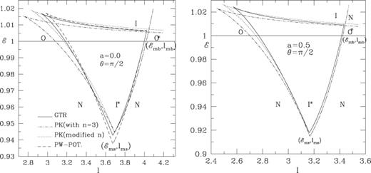
Panels (a and b): comparison of the parameter space spanned by specific energy and angular momentum in which multiple sonic points appear when the full GR consideration (solid curve), the PK potential with n= 3 (dash-dotted curve) and the PK potential with modified polytropic index (dotted curve), respectively, are used. Here, (a) a= 0 and (b) a= 0.5 have been chosen. Note that the overall agreement using the PK potential is much better when the modified n is used. For comparison, in (a), we have also plotted the boundary using the Paczyński–Wiita potential (long-dashed curve) for n= 3.
3 SONIC POINT CONDITIONS
The easiest way to solve the equations for radial dependence of velocity ϑ and sound speed a is to first obtain the sonic point conditions by taking the derivatives of energy and accretion rates with respect to x and eliminating d as/d x. We get
where a prime denotes the derivative with respect to x only and a subscript c denotes the quantities at the sonic point. In a black hole accretion, matter at the horizon must be supersonic (Chakrabarti 1990) and thus the flow must pass through a sonic point. At a sonic point, the denominator (D) vanishes and in order to have a finite velocity gradient throughout, the numerator must also disappear.
The vanishing of the numerator gives rise to the following condition:
Here, the subscript ‘c’ denotes a quantity at the sonic point. We define the Mach number as M= u/as then the Mach number at the sonic point is given by
Vanishing of the denominator (D= 0) yields the following condition:
Using the values of asc, the energy at the sonic point can be written as
As long as we use this PK approach, the velocity of the acoustic perturbation will remain  since this result is independent of the exact form of the pseudo-potential (see section 3.1.3 of Chakrabarti 1990). So the effective sound speed is
  and the true Mach number remains unity at the sonic points. However, when full GR considerations are used, one could choose the appropriate frame in which the Mach number is same as in equation (12). For instance, in Chakrabarti (1996b), where GR was used, the Mach number has the same form as equation (12) above, provided, radial velocity itself is measured in a rotating frame. Any other choice would have brought in explicit radial dependence in the Mach number at the sonic point. Another complicacy may arise from the definition of the vertical height itself. Chakrabarti (1996b) used the definition of Novikov & Thorne (1973) whereas Das, Bilić & Dasgupta (2006) used the definition provided by Abramowicz, Lanza & Percival (1997). Although the changes due to this choice are expected to be negligible, Das et al. (2006) found the radial dependence of the Mach number and they distinguished the sonic and critical points on the basis of this. A choice of radial velocity, e.g.
  to define the Mach number would have removed such a radial dependence.
In order to find out the number of locations (xc) where the sonic point conditions are satisfied, we have to study the energy variation as a function of xc for various angular momentum. In Figs 1(a) and (b), we plot these variations for the Kerr parameters (a) a= 0 and (b) a= 0.5. Different curves have been drawn for different specific angular momentum. From the top to the bottom curve, these are, (a) l= 2.6, 2.829, 3.0, 3.2, 3.4, 3.6, 3.8, 4.0 and (b) l= 2.3, 2.488, 2.7, 2.9, 3.1, 3.3, 3.5, 3.7, respectively. The dashed curves in both the cases are drawn for ‘critical’ angular momentum lc such that when the flow energy  is fixed, for l < lc, the number of sonic points is one, whereas for l > lc, the number of sonic points is three.
Energy at sonic points for (a) a non-rotating (a= 0) and (b) rotating (a= 0.5) black holes for various specific angular momentum using our PK potential. The curves are drawn for (from top to bottom), (a) l= 2.6, 2.829, 3.0, 3.2, 3.4, 3.6, 3.8, 4.0 and (b) l= 2.3, 2.488, 2.7, 2.9, 3.1, 3.3, 3.5, 3.7, respectively. The dashed curve in both the cases are drawn for ‘critical’ angular momentum lc such that when the flow energy  is fixed, for l < lc, the number of sonic points is one, whereas for l >lc, the number of sonic points is three.
In order to obtain a complete solution in the steady state, it is customary to obtain the velocity gradient at the sonic point and then use it to launch a stable procedure to integrate over the flow trajectory. Since the velocity gradient is indeterminate (=0/0) at the sonic point, we employ the L'Hospital's rule and obtain the following equations for the velocity gradient as
where
and

where

The velocity gradient at sonic point becomes
The nature of the two roots will determine whether the solution will be physical or unphysical. If the roots are real and of opposite signs then the sonic point will be of ‘saddle type’ and the solution would be physical (C90; Chakrabarti 1996a,b). If the derivatives are imaginary then the sonic points will be of ‘O’ type. In an inviscid flow as we are interested in this work, such sonic points will occur in between two saddle-type points.
In Figs 2(a) and (b), we plot the boundary of the parameter space spanned by the specific energy and angular momentum within which multiple sonic points are present (solid curve). This curve is drawn for (a) a= 0 and (b) a= 0.5 when the flow is on the equatorial plane. For  , there are three points whereas for
  , there are two sonic points, one saddle and one ‘O’ type. For comparison, we plotted the same parameter space as obtained by our potential when n= 3 is used (dash-dotted curve) and when the modified polytropic index n→n+ (0.3 − 0.2a) is used (dotted curve). The overall agreement with the modified polytropic index is much better. This is true for a < 0.8. For comparison, in Fig. 2(a), we plot the boundary (long-dashed curve) using the Paczyński–Wiita potential. The agreement is generally acceptable though it overpredicts the binding energy release (6.25 per cent as opposed to 5.7 per cent) as
  is lower than that in GR. Since the PK potential with the modified n agrees quite well we use this in future works on flows in vertical equilibrium. The physical reasons for the required modification of n is that the specific enthalpy in a relativistic flow is larger than n a2s[actually, including the rest mass, it is (1 −n a2s)−1]. One way could have been to increase the effective sound speed itself, but that would have increased the vertical height also, thus creating further deviations. The simplest way to enhance this term while still keeping ‘Newtonian’ form of specific energy is therefore to increase the polytropic index. In conical flows and flows of constant height, the mapping of n is not required as the sound speed can adjust itself when the Newtonian term is used. Since this adjustment does not affect the local vertical height, the results remain satisfactory.
4 LOCATIONS OF STANDING SHOCKS
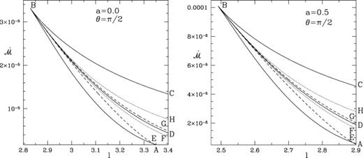
For a given energy and the specific angular momentum, the sonic points are obtained from equation (14). Using this and equation (7), we get the entropy accretion rate. In Figs 3(a) and (b), we plot the entropy accretion rate against energy as the sonic point is varied (see C89 for a similar study using the Paczyński–Wiita potential). The two curves are for (a) a= 0 and (b) a= 0.5. The sections AB and CD are drawn for ‘inner’ and ‘outer’ saddle-type sonic points whereas the section BC is drawn for ‘O’-type sonic points. The double-arrowed curves represent the direction in which the sonic point is increasing. Note that below M, where the curves intersect, the entropy at the inner sonic point is higher than the entropy at the outer sonic point and above M it is exactly the opposite. A shock formed in between these two saddle-type sonic points must combine two solutions with two different entropy densities, and the post-shock density must be higher for stability reasons (Zeldovich & Raizer 1968). Examples of such Rankine–Hugoniot shock transitions are shown by horizontal arrows s1, s2 and w1, w2, respectively: the first case represents a shock in accretion flows [see related discussion in C89 for shocks using the potential of Paczyński & Wiita (1980)], whereas the second case represents shocks in winds. At the shock x=xs, the conservation of energy flux across the shock gives

The conservation of the baryon number across the shock gives

and finally, the pressure balance condition across the shock gives
Here, W and Σ denotes the pressure and the density, respectively, integrated in the vertical direction as
and
where In= ((2nn!)2/(2n+ 1)!) and n being the modified polytropic index discussed above and ρe and Pe are densities and pressures on the equatorial plane, respectively.
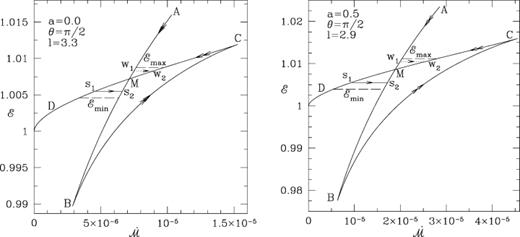
Entropy accretion rate is plotted against the specific energy as the sonic point is varied for a given specific angular momentum l: (a) a= 0 and (b) a= 0.5. The sections AB and CD are drawn for ‘inner’ and ‘outer’ saddle-type sonic points whereas the section BC is drawn for ‘O’-type sonic points. The double-arrowed curves represent the direction in which the sonic point is increasing. Examples of energy preserving shock transitions are shown by horizontal arrows: s1, s2 in accretion and w1, w2 in winds, respectively.
In Figs 3(a) and (b), the straight lines  and
and  represent the limits on the energy within which Rankine–Hugoniot conditions are satisfied. The curve is drawn for a given specific angular momentum marked inside the box. If
  or
or  , the conditions are not satisfied and no standing shocks can form. However, since two saddle-type sonic points are present, oscillations shocks could form in the accretion or wind flows (see Ryu, Chakrabarti & Molteni 1997 for the Paczyński–Wiita potential).
In Figs 4(a) and (b) (drawn for a= 0 and 0.5, respectively), the entire region of the parameter space is classified in the  versus l plane. Flows with parameters from the regions O (outer) and I (inner) have only one sonic point whereas those from the region ABC may have multiple sonic points. Inside the region ABD, the inner sonic point has more entropy than that at the outer sonic point and shocks (standing or not) may form only in accretion, while exactly the opposite situation occurs inside the region DBC where shocks (standing or not) may form only in winds. On the curve BD, the entropies at both the saddle-type sonic points are identical and no shock may form for the flow parameters which lie on this curve. It is clear that for a= 0.5 the shocks are produced as a smaller angular momentum and they are generally stronger and generate higher entropy at the shock. The locations of the standing shocks can be obtained by first obtaining the so-called ‘Mach number relation’ which correlates the Mach numbers before and after the shock. For standing non-dissipative shocks, this relation can be obtained from equations (19)–(21). This relation in independent of the nature of the pseudo-potential used. The derivation has already been given in C89 and we do not repeat it here.
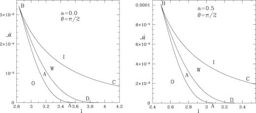
Classification of the parameter space in the  versus l plane (a) a= 0 and (b) a= 0.5. Flows with parameters from the regions O (outer) and I (inner) have only one sonic point whereas those from the region ABC may have multiple sonic points. In region A, the entropy density at the inner sonic point is higher than that in the outer sonic point while in W it is the other way round.
In Figs 5(a)–(d), we show four complete solutions (Mach number M as a function of radial distance x) for parameters marked inside the boxes. Each of these figures actually consists of two solutions passing through two sonic points, but only one truly connects the black hole horizon to infinity and the other is closed and connects either the horizon (Figs 5a and b) or the infinity (Figs 5c and d). These two distinct solution topologies are known as the X- and α-type topologies, respectively. In Figs 5(a) and (b), we show accretion solutions for a= 0 and 0.5 by an arrowed path. Here, the flow first passes through the outer sonic point ‘O’. The shock condition is satisfied at x and x (see C89 for nomenclature). After passing through the shock, the flow enters into the black hole through the inner sonic point located at ‘I’. The entropy that is generated at the shock is just the right amount to enable such a smooth passage through the inner sonic point. Figs 5(c) and (d) similarly contain typical solutions for winds coming out of discs in the (c) Schwarzschild (a= 0) and (d) Kerr (a= 0.5) geometry, respectively. Here, contrary to the earlier case, the solution first passes through the inner sonic point ‘I’ and then through the outer sonic point ‘O’ with the standing shock in between where the requisite entropy is generated. The pre- and post-shock flows are thus two solutions of perfect fluids with two different amounts of entropy accretion rates  . In Chakrabarti & Molteni (1993), while simulating the shocks of C89, it was discovered that only the outer shock is stable for accretion and the inner shock is stable for winds. We expect that the same conclusion will remain valid in this case as well.
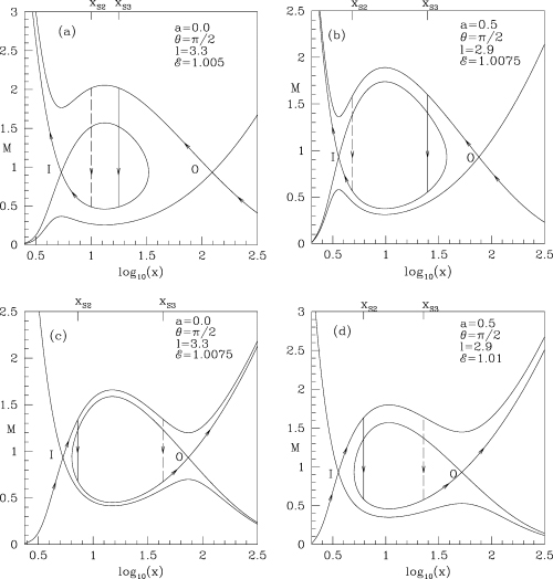
Panels (a–d): typical solutions which include shock waves are given in (a) and (b) for accretion and in (c) and (d) for winds. (a) a= 0; (b) a= 0.5; (c) a= 0 and (d) a= 0.5. The arrowed solid curve is the acceptable solution which includes a standing shock wave. The dashed line represents an unstable shock transition.
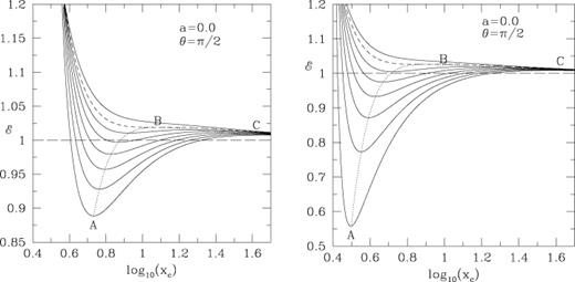
It may be relevant to check if the complete solution topology obtained using our PK potential is closer to that obtained from the GR. In Fig. 6(a), this comparison is done when the same polytropic index n is used. Here, the solid curves are for GR and the dotted curves are for the PK potential. The shock locations in these two methods are vastly different, xs3 | GR= 20.4 and xs3 | PK= 47.8. However, when we use the PK potential with modified polytropic index, the comparison is much better, xs3 | GR= 20.4 and xs3 | PK= 17.9. This is shown in Fig. 6(b). The parameters for which these solutions are drawn are:  and λ= 2.9. We believe that it may not be important to exactly match the properties for the same flow parameters. The relevant question is how closer the flow parameters are in two different methods so as to get similar results. We generally find that the variation of
  and λ is needed to get roughly the same result, that is, less than ∼5 per cent.

Comparison of the flow topologies and shock solutions with the full GR procedure (solid curve) when (a) the polytropic index n= 3 and (b) the modified polytropic index are used.
The shocks in the accretion flows play significant roles in determining the spectral properties as discussed in Chakrabarti & Titarchuk (1995) and Chakrabarti & Mondal (2006). Since the post-shock region is hotter, the hot, thermal, electrons can inverse Comptonize soft photons coming from the cooler pre-shock flow. Shocks can also accelerate electrons to produce non-thermal spectrum till very high energies. When the shocks are non-steady, oscillations of shocks can cause quasi-periodic oscillations of hard X-rays from black hole candidates (Chakrabarti et al. 2004). Thus, It is important to know how much region of the parameter space is actually available for the standing shocks and how much is available for the oscillating shocks. This is shown in (19)–(21) are not satisfied and hence the shocks are likely to be oscillating (see, Figs 7(a) and (b) for a= 0 and 0.5, respectively. In both the plots, AB, AD and AC have the same meanings as in Figs 4(a) and (b). The region within ABD is further divided by the curves BE and BF. The flow with parameters inside the region EAD will produce shocks in accretion and the post-shock region will have parameters inside the region FBD. Similarly, the flow with parameters inside the region DBG will produce shocks in winds and the post-shock flow will have parameters inside the region DBH. We generally note that as the Kerr parameter is increased, the shocks form at the lower angular momentum and they tend to generate higher entropies as the shocks become stronger and closer to the black holes. The regions ABE and GBC contain flow parameters which have more than one sonic points but the Rankine–Hugoniot relations such that the flows will have only the outer sonic point, only the inner sonic point, shocks in accretion, shocks in winds, ‘no-shocks’ in accretion and ‘no-shocks’ in winds, respectively (these latter two regions will have two saddle-type sonic points but the Rankine–Hugoniot conditions are not satisfied). The regions I*, O* and N contain parameters for which the flow will have only the inner α-type topology, outer α-type topology and no topologies at all. The solutions in the first two regions are incomplete and are not useful in an inviscid flow. In presence of viscosity, these α-type closed topologies open up and join with a solution reaching the boundary (1996a). Figs 8(a) and (b) show that as the Kerr parameter is increased, the region generally shrinks in the direction of the lower angular momentum and expands in the direction of the higher energy. We have already shown (Figs 4 and 7) that the shocks generate higher amount of entropy in the Kerr geometry.
Panels (a and b): subdivision of the parameter space presented in Figs 4(a) and (b) in terms of whether the shocks can form or not. (a) a= 0 and (b) a= 0.5. See text for details.
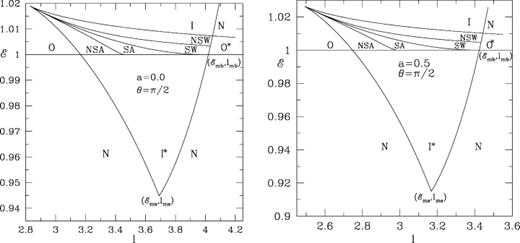
Panels (a and b): the subdivision of the parameter space spanned by  and l in terms of whether the multiple sonic points or shocks may form or not. The regions marked O, I, SA, SW, NSA and NSW contain flow parameters
  such that the flows will have only the outer sonic point, only the inner sonic point, shocks in accretion, shocks in winds, ‘no-shocks’ in accretion and ‘no-shocks’ in winds, respectively. In regions I* and O*, only the inner and outer α-type topologies are possible. In region N, no solution is possible. (a) a= 0 and (b) a= 0.5. The subscripts ‘mb’ and ‘ms’ refer to marginally bound and marginally stable values, respectively.
Using the procedure same as in C89, one can compute the shock locations. For a given set of flow parameter  , there are two shock locations x and x (using the notation of C89) in between the inner (xi) and outer (xo) sonic points: xo > x > x > xi. Out of these two shocks, our numerical simulations show that the inner one is stable for winds and the outer one is stable for accretion. The results of the simulations will be reported in the next paper of this series. In Figs 9(a) and (b), we present the variation of the shock location (along the y-axis) as a function of the energy (along the x-axis) and the angular momentum (marked on each curve). The solid curves are for the accretion flow parameters taken from the SA in Figs 8(a) and (b), whereas the dotted curves are for the wind flow parameters taken from the region SW in those figures. In Figs 9(a) and (b), a= 0 and 0.5 were chosen. For a given energy, the shock occurring closer to the black hole (x) is stable for winds (dotted curve). The shock occurring away from the black hole (x) is stable only for accretion. Note that when the black hole is rotating, the shocks can form closer to the black hole and for a very low angular momentum.
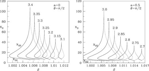
Variation of the (a and b) inner shock xs2 and outer shock xs3 (along the y-axis) as a function of the energy (along the x-axis) and the angular momentum l (marked on each curve). The solid curves are for the accretion flow parameters taken from the SA in Figs 8(a) and (b), whereas the dotted curves are for the wind flow parameters taken from the region SW in those figures. (a) a= 0 and (b) a= 0.5. Only outer shocks drawn in solid curves and inner shocks drawn in dotted curves are found to be stable.
5 CONCLUDING REMARKS
In Paper I of this series, we presented a modified gravitational potential. Particles moving in this potential behave as though they move around a Kerr black hole. In this paper, we used this so-called PK potential to show that as far as the transonic flow properties are concerned, a flow in the PK geometry reproduces similar behaviour to that of the Kerr geometry (Chakrabarti 1996b). In this paper, we have generalized our work on the properties of standing shocks in an accretion flow of the constant specific angular momentum. Instead of using Paczyński & Wiita (1980) potential which mimics the Schwarzschild geometry, we used a potential which is tested to mimic the Kerr geometry quite accurately for a < 0.8. For fluid dynamical computation, the polytropic index requires a correction when the flow height depends on its temperature. We subdivided the parameter space in regions which produce standing and oscillating shock waves. We also compute the variation of the locations of the shock waves with the specific angular momentum and energy. We note that as the spin of the black hole is increased, accretion shocks can form even for very low specific angular momentum, though the energy required is higher.
The use of the pseudo-Newtonian potential has reduced the complex problem of finding non-linear solutions such as shocks in a black hole geometry into a much simpler problem. It allowed us to assume that the specific energy could be written as a sum of a few linear terms. In future, we will use this to conduct numerical simulations to check if these shocks remain stable or they oscillate. We anticipate that in the regions of the parameter space in which the standing shock conditions are not satisfied, the shocks would oscillate exactly as in the case of non-rotating black holes. Since the oscillation time-scale is proportional to the infall time-scale from the shock (MSC96), as the shocks form closer to the black hole, the frequency of oscillations will also increase. Earlier, suggestions were made that these shock oscillations may cause quasi-periodic oscillations in X-rays in black hole candidates (MSC96, CAM04). The presence of high-frequency QPOs of X-rays as observed in several stellar black hole candidates could thus be indicative of oscillations of shocks which are formed around a spinning black hole.
Another important problem is to see if there are subtle differences between the high-energy spectrum of a spinning black hole and a non-rotating black hole. Since the post-shock region could be very hot, the electrons in this region will behave as a Comptonizing cloud and energize the soft-energy photons to higher energy through inverse Comptonization. Additional complicacy arises due to the creation of a non-thermal electron distribution at the shock which will generate power-law synchrotron radiation, which in turn could also be inverse Comptonized. The computation of the spectrum around Kerr black holes is under way and will be reported elsewhere.
