


Abstract
The effect of photon-beam-induced turbulence on the propagation of radio emission in a pulsar magnetosphere is discussed. Beamed radio emission with a high brightness temperature can generate low-frequency plasma waves in the pulsar magnetosphere, and these waves scatter the radio beam. We consider this effect on the propagation of radio emission both in the open field line region and in the closed field line region. The former is applicable to most cases of pulsar radio emission where the propagation is confined to the polar region; it is shown that the induced process is not effective for radio emission of moderately high brightness temperature but can have a severe effect on giant pulses. For giant pulses not to be affected by this process, they must be emitted very close to the light cylinder. We show that the induced process is efficient in the closed field line region, inhibiting propagation of the radio emission in this region.
1 INTRODUCTION
It is generally thought that pulsar radio emission is produced in the open field line region (OFLR) well inside the light cylinder (LC) (the radius at which the corotation speed equals c). Radio emission generated inside the LC must propagate over a substantial part of the magnetosphere before escaping to the interstellar medium. The intense radio emission is subject to various interactions with the intervening plasmas within the pulsar magnetosphere. Two types of interactions have been considered: cyclotron absorption in which electrons (positrons) are in cyclotron resonance with the wave (Blandford & Scharlemann 1976; Fussell, Luo & Melrose 2003), and induced Compton scattering in which the radio wave is scattered to a higher or lower frequency (Blandford & Scharlemann 1976; Petrova 2004a). Both the processes can affect or even disrupt the propagation of the beam. So far, no clear observational evidence for the absorption feature associated with the cyclotron resonance has been identified. However, the conventional polar cap theory, which assumes that the radio emission is generated in an outflowing electron–positron pair plasma, does predict a cyclotron resonance region where absorption should occur. Induced Compton scattering can be important in principle for any coherent emission with a sufficiently high intensity (Wilson & Rees 1978; Sincell & Krolik 1992; Coppi, Blandford & Rees 1993; Hardy & Melrose 1995). While cyclotron absorption is important only in the region near the LC, induced scattering can occur throughout the magnetosphere. Apart from these two processes, there is a third process that involves induced wave–wave interactions and that can significantly affect the propagation of the radio beam. A highly collimated beam of radio waves can generate low-frequency waves through three-wave interactions in the pulsar magnetospheric plasma in a way similar to wave generation in a particle beam instability. These low-frequency waves interact with the radio waves, leading to a decrease in its intensity and an increase in its angular spread. In some cases, such effects can completely disrupt the radio beam: the medium becomes opalescent to the radio waves.
In this paper, we discuss the effect of induced three-wave interactions on the propagation of radio emission in a pulsar magnetosphere. Induced three-wave processes have been considered for pulsar winds (Luo & Melrose 1994), pulsar eclipse by the stellar wind of its companion (Melrose 1994; Thompson et al. 1994; Luo & Melrose 1995) and radio emission from active galactic nuclei (Krishan 1988; Gangadhara & Krishan 1993; Levinson & Blandford 1995). Apart from a discussion of Raman scattering (a particular case of three-wave interactions; cf. Section 2.5) in a pulsar magnetosphere (Gangadhara & Krishan 1993; Lyutikov 1998), we are aware of no detailed study of the three-wave effect which explicitly takes account of the beaming and broad-band nature of the radio emission. To our knowledge, there is no detailed study of propagation of radio emission in the closed field line region (CFLR). Here, we consider the three-wave effect both in the OFLR and in the CFLR. In most models, propagation of radio emission is confined to the OFLR where the relativistic electron–positron pair plasma streams along magnetic field lines at a relativistic velocity. Because electrons and positrons contribute to three-wave interactions equally but with opposite sign, three-wave interactions are significantly weakened in a quasi-neutral pair plasma. However, such processes can still be important for radio emission with very high brightness temperature provided that there is a modest excess of electrons or positrons and that the bulk Lorentz factor is modest. Since for young pulsars, the conventional polar cap model generally predicts a plasma density too high for the propagation of radio waves, we assume that the plasma is highly inhomogeneous across the polar cap and that radio emission is generated at a frequency near the plasma frequency (in the plasma's rest frame) in the underdense region where the plasma density is relatively low (cf. Section 3.1). This assumption seems to be required for consistency if the radio emission is produced due to a beam instability (Melrose & Gedalin 1999).
Propagation of radio emission in the CFLR is relevant at least for three specific cases: (i) the recently discovered double-pulsar system PSR J0737−3039B in which the radio emission from one pulsar interacts with the plasma in the CFLR of the other, (ii) radio emission from outer magnetospheric regions where the emission of the trailing component may propagate to the CFLR as a result of the aberration effect and (iii) backward emission predicted by the oscillatory polar gap model (Levinson et al. 2005) and by recent models for the peculiar ‘notch-like’ feature of pulse profiles (Dyks et al. 2005). For case (i), eclipse of the radio emission from one pulsar by the magnetosphere of the other has been observed. A possible interpretation of the eclipse is due to processes in the CLFR such as cyclotron or synchrotron absorption or induced scattering. For case (ii), the trailing component may have an absorption-like feature or may be completely destroyed as the result of strong induced processes. For the third case, induced processes can severely constrain visibility of the backward emission that propagates through the CFLR.
In Section 2, we outline a general formalism of induced three-wave interactions in the pulsar magnetosphere. We discuss the effect on propagation of radio emission in the OFLR in Section 3 and in CFLR in Section 4.
2 INDUCED THREE-WAVE INTERACTIONS
We consider three-wave processes due to passage of beamed radio emission (referred to as a photon beam or radio beam). The processes involve two high-frequency waves (unscattered and scattered radio waves) and a low-frequency wave generated by the radio beam. The three waves satisfy the resonance conditions ω↔ω′+ω″ and k↔k′+k″. The condition ω∼ω′≫ω″ means that three-wave scattering is approximately ‘elastic’.
2.1 Three-wave probability
We model pulsar radio emission as a highly collimated photon beam, described by the photon occupation number N(k), where ω is the wave frequency and k is the wave vector. The photon occupation number is a Lorentz invariant, related to the brightness temperature Tb through  , where kB is the Boltzmann constant. Let NL(k″) be the occupation number of the low-frequency wave with frequency ω″ and wave vector k″. Evolution of N(k), N(k′) and NL(k″) is done by three kinetic equations which are completely determined by the three-wave probability (Melrose 1986): W(k, k′, k″)(2π)4δ(k−k′−k″)δ[ω(k) −ω′(k′) −ω″(k″)], where the delta functions are the three-wave resonant conditions and
In (1), which is simply referred to as the three-wave probability, αijs is the quadratic response tensor, RL is the ratio of the electric to total energy of the low-frequency wave and the polarizations of three waves are e, e′ and e″. In deriving the three-wave probability, we adopt the cold plasma form for the quadratic response tensor, e.g. equation (A1) in Luo & Melrose (2006), and take the strong magnetic field limit. One should note that the strong field limit may not be appropriate for the region near the LC. None the less, it allows us to simplify the quadratic response tensor greatly. In this limit, one finds that the dominant component is the projection to the magnetic field, denoted by α∥, given by
where ω≈ω′≫ω″, ωp is the plasma frequency, n∥=k∥c/ω, n′∥=k′∥c/ω′, n″∥=k″∥c/ω″, η is the ratio of the difference to the sum of the positron and electron number density, with η=−1 corresponding to an electron gas. We use the subscript ∥ to denote the parallel (to the magnetic field) component. The final expression for the three-wave probability is
where re=e2/(4πɛ0mec2) ≈ 2.8 × 10⁻¹⁵ m is the classical electron radius and ξp= (ωp/ω″)1/2 (n∥+n′∥−n″∥)e∥e′∥e″∥. The expression (3) is closely analogous to a similar expression for an unmagnetized plasma (Melrose 1994) where the low-frequency waves are the Langmuir waves (ω″=ωp). For a quasi-neutral, cold electron–positron plasma, one has η= 0; one then needs to retain higher order terms in an expansion in (ω, ω″)/Ωe≪ 1 to obtain a non-zero three-wave probability, which is much smaller than (3) (Luo & Melrose 1997).
In the following, we consider two low-frequency modes that may be relevant to induced three-wave interactions: the Langmuir mode that propagates along the magnetic field, and the Alfvén mode (also called the low-frequency LO mode) which can propagate at any direction. Note that the three-wave process involving a Langmuir wave in the (coherent) fixed-phase formalism is also called stimulated Raman scattering (cf. Section 2.5). Landau damping imposes a lower limit to the wavelength of low-frequency waves. To determine the Landau damping, one needs to separately consider an intrinsically relativistic plasma such as in the OFLR and a non-relativistic plasma such as in the CFLR. Landau damping in an intrinsically relativistic plasma occurs preferentially for n″∼ 1 since the plasma is relativistic even in the plasma rest frame, and the particle's Cerenkov resonance occurs for the wave phase speed near the speed of light. In the non-relativistic plasma, Landau damping is effective for electrostatic waves with n″∼n″max= 0.3c/λDωp (where λD is the Debye length) (Bekefi 1966), leading to a limit on the maximum n″max≫ 1. Since |ξp|2∝n″2, three-wave interactions involve low-frequency electrostatic waves and should be important in the CFLR where the plasma is expected to be non-relativistic (cf. Section 4.1). In the OFLR, the plasma is intrisically relativistic, Landau damping limits the refractive index of the Langmuir waves to about 1 and both the Alfvén and electrostatic modes need to be considered.
2.2 Scattering rate
We consider the production rate of scattered photons as a measure of the effect of the three-wave process on the photon beam. This rate, which we also call the scattering rate, depends on the level of the low-frequency waves generated by the photon beam. We consider the case where the low-frequency waves are saturated as the result of change in the occupation number of the photon beam. The saturation condition dNL/dt= 0 leads to a level of low-frequency waves expressed in terms of the photon occupation number. Thus, the scattering rate can be written as
where ΔΩ is the angular spread of the photon beam. Our specific model for an axially symmetric beam is
where ΔΩ= 2πΔΘ20, ΔΘ0≪ 1 is the beamwidth and the polar angles (Θ, Φ) are defined with respect to the beam axis. Similarly, we use (Θ″, Φ″) for the polar angles of k″. The polar angles of k and k″ relative to the magnetic field (z-axis) are given, respectively, by (θ, φ) and (θ″, φ″). Since the angular spread of the beam is small, hereafter we do not distinguish between the beam axis and k. Substituting (3) for (4) yields
where we express the incoming photon occupation number in terms of the brightness temperature: , and ξp depends on the specific low-frequency mode involved and is derived in Sections 2.3 and 2.4.
From (6), one may define the opacity for the photon beam propagating over a distance Δs:
In (7), ΔΩTb can be estimated from the observed flux density Sobsν:
where ν≡ω/2π is the frequency in Hz, Δs is the distance from the emitting region to the region concerned and DL is the pulsar distance. If one assumes that the size of the emission region is δl, one has ΔΩ∼ (δl/Δs)2. The brightness temperature is estimated to be Tb∼ 5 × 1028 K for δl= 102 m.
2.3 Back scattering
Consider first the case where the low-frequency waves are Langmuir waves propagating along the magnetic field at a low phase speed ω″/k″≪c (or n″≫ 1). Three-wave interactions favour the back scattering regime where the incoming and scattered photons propagate in opposite directions. From the three-wave resonance conditions, one has k∥=k′∥+k″ (parallel to the magnetic field) and k⊥=k′⊥ (perpendicular to the magnetic field), which gives rise to cos θ≈ cos θ′+n″(ωp/ω), where n=kc/ω≈n′=k′c/ω′≈ 1 and ω″=ωp. Because of k≈k′, one must have θ′∼π−θ, corresponding to the incoming and scattered photons propagating in opposite directions. Hence for Langmuir waves, one derives
provided that 2 cos θ(ω/ωp) < n″max, where n″max is determined by the Landau damping. The angular range for back scattering to occur is cos θ≤ min{1, k″max/2k} with k″max=n″maxωp/c. When the photon beam is parallel to the magnetic field, one has |ξp|2∼ (ω/ωp)2(ΔΩ/π)2, which implies that only photons off the beam axis with θ≠ 0 can interact with the Langmuir waves. In a non-relativistic plasma, one has n″max≫ 1, and hence the back scattering can be very efficient.
2.4 Diffusion of the photon beam
In the regime k″≪k∼k′, the three-wave interactions resemble particle–wave interactions, with high-frequency waves (the radio emission) acting like ‘particles’ that can emit or absorb low-frequency waves (Melrose 1994; Luo & Melrose 1995, 1997). This regime is also called the small angle scattering because the angle between the incoming and scattered photons is small, given by θkk′≈k″/k≪ 1. The three-wave resonance conditions reduce to the Cerenkov resonance condition between ‘particles’ (the high-frequency wave) with a velocity vg=∂ω(k)/∂k and a wave with (ω″, k″). Specifically, one may define a Cerenkov angle χ0=arccos(ω″/k″c), corresponding to a conical surface with respect to vg, which defines the Cerenkov resonance condition. The condition can only be satisfied for a subluminal wave n″=k″c/ω″ > 1, i.e. its phase speed must be less than c. We are interested in negative absorption (or growth) of the low-frequency waves, which occurs for Θ″∼χ0−ΔΘ0, at a rate determined by the three-wave probability (1) or (3) (Luo & Melrose 1997).
The instability of low-frequency waves leads to diffusion of photons in the k-space, determined by the diffusion coefficient Dij∝k″2k″ik″jWNL/c, where the three-wave probability W is given by (1). The growth of low-frequency waves is entirely due to the anisotropic angular beaming of the photons. A decrease in the beaming, over the perpendicular diffusion time t⊥=k2⊥/D=ΔΩk2/D, where  , is especially important as it can ultimately suppress the growth. Assuming that the low-frequency waves are saturated due to perpendicular diffusion, one can derive the total diffusion time td=k2/D= 1/Γ, which describes the effect of the instability on the beam. One finds Γ is the same as that given by (4) or (6) (Luo & Melrose 1995) and the diffusion effect can be estimated by evaluating the opacity (7). For Langmuir waves, one finds
where 1 < n″≪ω/ωp. Similarly for Alfvén waves, one has
where the parallel component of the polarization is |e″∥| ≈ (ω″/ωp)2n″ sin θ″≪ 1, θ″ < 1 and n″∥≈ 1 (Arons & Barnard 1986; Melrose & Gedalin 1999).
2.5 Induced Compton scattering
The relation between the induced three-wave interaction discussed here and induced (or stimulated) Compton scattering requires comment. (We use ‘induced’ and ‘stimulated’ interchangeably here.) Both processes need to be considered in discussing the propagation of radiation with very high brightness temperature, and we regard them as independent of each other. In our view, the difference between these two processes has become somewhat obscured by discussions of stimulated Raman scattering. Formally, Raman scattering is associated with particles (atoms or molecules) that have an intrinsic transition frequency, say ωR, associated with them. Spontaneous Raman scattering of incident radiation with frequency ω produces scattered radiation at the Stokes frequency, ω−ωR, and at the anti-Stokes frequency, ω+ωR. Stimulated Raman scattering is analogous to absorption of the beat between the incident and scattered radiation, and occurs at a rate that is proportional to the product of the intensities at the incident and the scattered frequencies. This leads to exponential growth at the Stokes frequency, and an associated exponential decay at the incident frequency, so that radiation is transferred from higher to lower frequency at an exponentially increasing rate. (If the scattering particles have an inverted energy distribution, negative absorption or maser action results in an exponentially increasing transfer from the incident frequency to the anti-Stokes frequency.)
Induced Compton scattering is analogous to induced Raman scattering, except that there is a continuum of frequencies for the scattered radiation. For isotropic radiation with a peak in the intensity at some frequency, induced Compton scattering tends to move this peak to lower frequencies; if there are two distinct beams of radiation, induced Compton scattering tends to transfer radiation from the beam at the higher to the beam at the lower frequency. The direction of transfer is reversed if the scattering particles have an inverted energy population, and this has been suggested as a mechanism for generating giant pulses (Petrova 2004b). The induced three-wave interaction discussed here is essentially the same process described as ‘stimulated Raman scattering’ by Gangadhara & Krishan (1993) and as ‘induced Raman scattering’ by Lyutikov (1998) except that in our case the low-frequency wave is not restricted to plasma waves. The important distinction, as noted by Lyutikov (1998), is that in the induced three-wave interaction, the Raman frequency, ωR, is replaced by the frequency of the low-frequency waves, which is the plasma frequency, ωp, in cases of interest. However, this analogy is only kinematic, and the dynamics of the two processes are quite different; for example, they are described by different kinetic equations. In the induced three-wave interaction, the plasma may be regarded as passive, determining the wave dispersion and the non-linearity that allows the three-wave coupling. The kinetic equation involves on the wave distributions: the low-frequency waves grow and result in the scattering of the high-frequency waves. In contrast, in induced Compton scattering, the plasma particles actively scatter the high-frequency waves, the process depends explicitly on the distribution function for the particles, and no low-frequency wave is involved.
3 PROPAGATION IN THE OFLR
The formalism derived in the preceding section can be applied to the case of propagation of radio emission in the OFLR where the plasma has a bulk velocity v=βc and a Lorentz factor γ= 1/(1 −β2)1/2. A convenient approach is to treat the formalism in Section 2 in the plasma rest frame and then derive the relevant quantities in the pulsar or observer's frame by a Lorentz transformation. Note that some caution is needed in defining the bulk rest frame. Since the plasma streams along curved magnetic field lines, there is no single bulk frame. However, one can still construct a consecutive series of local bulk frames along the curved field lines, an approach similar to that used in ray tracing in a relativistically flowing plasma (Fussell & Luo 2004). We assume that the photon beam is axially symmetric in the plasma rest frame. The photon beam shape varies from frame to frame. Such complication is not considered here, though it should be included in a full radiative transfer calculation. Specifically, the relevant propagation angle is transformed according to
All tilde quantities correspond to the rest frame. We ignore the pulsar's rotation in the Lorentz transformation. The brightness temperature, frequency, differential solid angle and plasma frequency are transformed according to  and
and  , where the refractive index is n≈ 1. Since the time derivative in (4) is interpreted as the total time derivative, i.e. d/dt=∂/∂t+cn·∇ with n=k/k, one has
  (Pomraning 1973; Hardy & Melrose 1995; Sazonov & Sunyaev 1998). Upon making the Lorentz transformation, one obtains the scattering rate in the observer's frame:
where M is the pair multiplicity. In (13), we use η= 1/2M and rewrite the plasma frequency as ωp= (2M)1/2ωpe, where ωpe is the plasma frequency corresponding to the number density of the excess electrons or positrons.
3.1 Plasma density
The scattering rate is proportional to the local net charge density: a higher net charge density implies a faster scattering rate. This is due to the electrons and positrons contributing with opposite sign to the three-wave coupling coefficient. For the conventional polar cap model, the number density of the excess charge is the Goldreich–Julian (GJ) density, given by nGJ≈ 7 × 10¹⁷ m−3 (P/0.1 s)−1 (B/108 T)(R0/r)3 (Goldreich & Julian 1969), where R0= 104 m is the star's radius. Seemingly insurmountable difficulties arise if one assumes the most widely discussed emission mechanism (a beam instability) in a plasma with the GJ density times a multiplicity M≥ 1. The lowest frequency consistent with theory is ωc∼ 2(γ/〈γ′〉)1/2ωp (Melrose & Gedalin 1999), where 〈γ′〉 is the Lorentz factor's mean spread in the plasma rest frame, about 1–10 (Arendt & Eilek 2002). In the following, we assume 〈γ′〉= 4 implying ωc=γ1/2ωp. For example, the plasma frequency predicted for the Crab pulsar is ωp≈ (2 × 10¹² s−1 )(R0/r)3/2 (M/100)1/2, corresponding to ωc∼γ1/2ωp≈ (2 × 10¹³ s−1)(R0/r)3/2 (M/100)1/2 for γ= 100, which is too high compared with the observed frequency. [This plasma density problem was discussed by Kunzl et al. (1998).] One practical solution to this problem is that the plasma is highly inhomogeneous forming underdense regions where radio emission is produced and propagates. The low-density region where the density is actually much lower than 2MnGJ can form as a result of non-uniform extraction of primary particles from the polar cap or non-uniform pair cascades (Levinson et al. 2005). In the former case, the primary particle density is non-uniform across the polar cap forming localized outflowing fluxes along field lines separated by low-density regions where the net charge density is much less than nGJ (though on average the mean flux density from the polar cap is still nGJc). Both the multiplicity M and the net charge density can be low in the underdense region.
In the following, we consider the case where the radio wave is emitted in the low-density regions at a frequency near the local plasma frequency. Specifically, we assume (i) the radio frequency is ω∼ωp*γ1/2, where  is the local plasma frequency at the emission radius r* and
  is the mean multiplicity, and (ii)
  is a constant along the propagation path. Assumption (i) is applicable if the coherent radio emission is due to wave–particle interactions (Melrose & Gedalin 1999). Although assumption (ii) may not be realistic, particularly in the oscillatory case where both the multiplicity M and the net charge density can be non-stationary (Levinson et al. 2005), it is a reasonable approximation provided that the size the scattering region (r*/γ) is much larger than the length-scale (corresponding to the polar gap length) of plasma inhomogeneities along the propagation path. These two assumptions allow us to estimate (13) without going into much details on a particular polar cap model. We consider the following three propagation regimes separately: two quasi-parallel regimes, including the forward propagation
  and backward propagation
  , and quasi-perpendicular regime
  .
.
3.2 Quasi-parallel propagation
In the forward propagation regime,  is nearly parallel to the magnetic field. Assuming the low-frequency plasma wave propagates along the magnetic field, one has
  and
and  . We assume that the photon beam is in the LO mode with the polarization in the B–k plane, because only this high-frequency mode can be produced through wave–particle interactions (Melrose & Gedalin 1999). If one assumes that the radio emission is generated near the frequency ω∼ωp*γ1/2 at the emission radius r*, the plasma frequency in the rest frame is comparable with the photon frequency. Thus, the only relevant low-frequency waves are Alfvén waves.
For the Alfvén mode, one can show that three-wave interactions due to the projection of the polarizations of all three waves along the magnetic field are small. From (11), which applies in the rest frame, one obtains  , where
  . For
. For  and
and  , one has
  .
.
In most part of its propagation path, the radio emission propagates backward in the rest frame, as indicated in (12), one has  for θ≫ 1/γ, i.e. the emission propagates backward (
 ) in the rest frame. In the rest frame, the frequency is given by
  . Since ω∼ωp*γ1/2, one has
  or
or  , where
  for Δs/r*= (r−r*)/r* < 1. Thus, for backward propagation, the Langmuir waves can be treated as low-frequency waves (
 ) and back scattering (cf. Section 2.3) is allowed kinematically but is inhibited by the Landau damping. For backward propagation, the LO mode is elliptically polarized, with only a small component along the magnetic field |e∥| ≈ |e′∥| ≈ 2/θγ≪ 1. From the three-wave resonance conditions, one finds
  Fig. 1, and in this regime the low-frequency approximation is justified. From. However, Landau damping limits the refractive index to
  .
.
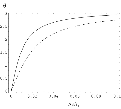
Propagation angle in the rest frame versus propagation distance Δs/r*. The propagation angle  , which is assumed to start from zero (at Δs= 0), rapidly increases to π after a distance Δs=r−r* > r*/γ. A dipole magnetic field is assumed. The solid and dashed lines correspond to γ= 100 and 50, respectively.
For backward propagation, the three-wave interaction can proceed in the regime k″≪k∼k′ where both Langmuir and Alfvén waves are relevant. From (10), one obtains  for the Langmuir waves with
  and from (11) one has
  for the Alfvén mode. Thus, Alfvén waves are less efficient than Langmuir waves.
3.3 Quasi-perpendicular regime
The transition between forward and backward propagation,  , in the rest frame corresponds to θ∼1/γ in the pulsar frame. A photon beam that is emitted initially along the magnetic field rapidly acquires an angle as the magnetic field lines bend away (cf. Fig. 2). The propagation enters the quasi-perpendicular regime (
 ) after the distance Δs∼r*/γ. Similar to forward propagation, the plasma frequency is comparable with the radio frequency in the rest frame. So, the plasma waves cannot be treated as low-frequency waves. The relevant low-frequency waves are the Alfvén waves. From (11), we have
  . Although the process favours a higher ω″, the Alfvén mode is heavily damped near the plasma frequency. It can freely propagate in the range
  . For example, one may choose
  and
and  . This gives
  .
.
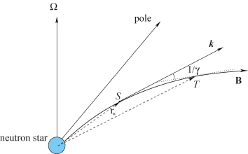
Propagation of the photon beam emitted at r*. The propagation enters the quasi-perpendicular regime at T where the propagation angle in the pulsar frame is θ∼1/γ. The distance from the source (S) (at r*) to the quasi-perpendicular regime (T) is approximately r*/γ.
To calculate (13), we determine the plasma frequency in the propagation path from ωpe=ωp/(2M)1/2=[ω/(2Mγ)1/2](r*/r)3/2 with r∼r* in the quasi-perpendicular region. Note that for young pulsars such as the Crab pulsar, the local plasma frequency determined in this way is much lower than the one derived from the density  (cf. Section 3.1). The opacity τ=ΓΔs/c=Γr*/γc is estimated as
where (8) with Δs=r*/γ is used. It should be noted that if the emission is from a region spread over r*/γ, the opacity estimated from (14) is reduced. If one assumes the nominal value  for typical pulsar parameters, equation (14) shows that the induced diffusion is not important for radio emission with a moderately high brightness temperature. However, it can be effective for young pulsars or pulsars that emit giant pulses.
3.4 Giant pulses
For giant pulses, the opacity (14) can well exceed unity and as a result, it imposes a severe constraint on their propagation. Giant pulses have been observed from a few pulsars with the two best examples being the Crab pulsar (Lundgren et al. 1995; Hankins et al. 2003), a fast rotating young pulsar, and PSR 1937+21 (Kinkhabwala & Thorsett 2000), the second fastest millisecond pulsar. The distribution of pulse energy (the flux density times the typical pulse width) is power law, in contrast to normal radio pulses that have a log-normal distribution (Romani & Johnston 2001). This implies that the emission mechanism for giant pulses is distinct from that for normal radio pulses. Although the emission mechanism for giant pulses is not well understood, recent study of giant pulses in relation to the corresponding high energy emission suggests that the emission region may be in or near the outer magnetospheric region where the high energy emission originates (Romani & Johnston 2001). Here, we show that the opacity constraint (14) excludes the possibility of giant pulses originating from the inner magnetosphere and deduce that they must come from the outer magnetosphere, near the LC.
The opacity (14) decreases with increasing emission radius. This feature can be understood as follows. The efficiency of induced three-wave processes depends on the photon energy density. For an emitting source of size δl, the photon energy density in the quasi-perpendicular region (at a distance r*/γ from the source) is proportional to (δl/r*)2kBTb. Observations of nanosecond giant pulses from the Crab suggest a source size of the order of a metre (Hankins et al. 2003). This density decreases with increasing r*, leading to a weakening of three-wave interactions. For giant pulses from the Crab pulsar, one has an average flux density Sobsν∼103 Jy. We have τ≫ 1 unless a large emission radius r* is assumed. For giant pulses not to be strongly affected by the induced process, corresponding to the condition τ < 1, the emission radius must satisfy the condition
where  . Although the pair multiplicity is not well constrained, (15) still gives a strong constraint on the emission radius for a reasonable parameter range. A recent numerical simulation suggests that the conversion efficiency of the primary particle energy to pairs is well below unity (Arendt & Eilek 2002), corresponding to
  , where γb is the primary particle's Lorentz factor. For young pulsars, resonant inverse Compton scattering is the dominant emission process for pair-producing photons and it is reasonable to assume γb∼105. This gives an upper limit
  . Applying (15) to the Crab pulsar, assuming a distance
  and γ= 102, one finds r* > 5 × 10⁵ m, about 0.3 of the LC radius RLC≈ 1.6 × 10⁶ m. One concludes that for giant pulses to propagate without being dispersed by induced three-wave interactions, they must be emitted very close to the LC radius. For the millisecond pulsar PSR 1937+21, one expects M to be small and γ to be large as pair production in the millisecond pulsar's magnetic field is much less efficient. Assuming that the primary particle's energy is limited by curvature radiation corresponding to γb∼107, one has the upper bound Mγ < 5 × 10⁶. For example, for DL= 3.6 kpc, M= 10, γ= 105 and Sobsν= 300 Jy, one has r* > 3 × 10⁴ m, about half the LC radius.
4 PROPAGATION IN THE CFLR
The formalism discussed in Section 2 can be directly applied to the CFLR where the plasma consists of single-sign charged particles with the GJ density nGJ and is stationary with a zero bulk velocity. All the relevant quantities discussed in Section 2 are now referred to the pulsar frame.
4.1 Plasmas in the CFLR
In contrast to the polar region, the plasma in the CFLR is plausibly stationary in the corotating frame. Since particles are in the ground Landau state, they do not have a perpendicular momentum, so there is no magnetic mirror effect that can trap a dense plasma. This feature is very different from the usual planetary magnetosphere in which a plasma is trapped due to this effect. Thus, in the absence of continuous injection of pairs the plasma density in this region is controlled by the pulsar's rotation in such way that the charge density is enGJ (Goldreich & Julian 1969). The plasma in this region consists of particles with a single sign of charge (electrons or positrons or possibly protons), which can be treated as an electron gas in one dimension (along the field lines). Assuming the magnetic field as a function of radius r: B∝ (R0/r)δ, where δ= 3 for a magnetic dipole, one may express the density as ne=nGJ(R0/r)δ. Using (7) and (6), one obtains
where ξp is given by (9) for back scattering and (10) for the quasi-linear diffusion approximation. Note the difference in the radial distance dependence in (16) compared to (14). This difference is due to the GJ density varying with radial distance proportional to the magnetic field, where we ignore a cosine factor. The CFLR region is separated into a positive charge region and a negative charge region, with the boundary between them called the null surface. One may define a radius rcr where τ= 1. The opaque region corresponds to r≤rcr, where induced three-wave processes are important. This critical radius is derived as
We are interested in the region sufficiently far from the star's surface such that the condition ω≫ωpe is satisfied. We discuss only the case where the low-frequency waves are electrostatic.
4.2 Eclipse in the binary pulsar J0737−3039B
We first apply (16) to the double-pulsar system J0737−3039B, in which radio emission from one pulsar is periodically eclipsed by the other. It is of interest to consider if induced scattering can provide an effective mechanism for such eclipse. The system consists of pulsar A with the period 22.7 ms and magnetic field 6.3 × 10⁵ T, and pulsar B with the period 2.8 s and magnetic field 1.6 × 10⁸ T. The two pulsars are in a nearly circular orbit (with the eccentricity 0.088), with the orbital plane seen nearly edge-on, at an inclination angle ∼87° to the line of the sight (Lyne et al. 2004). Observations indicate that the nearest impact distance of the photon beam from pulsar A to pulsar B is about 0.1RLC− 0.2RLC (of pulsar B). The plasma frequency at r= 0.1RLC is about ωpe≈ 2 × 10⁵ s−1. Cyclotron absorption is probably unimportant because the plasma density is too low (Lyutikov & Thompson 2005).
Consider interaction of a photon beam from pulsar A with the magnetospheric plasma of pulsar B. The brightness temperature of the radio emission from pulsar A is estimated to be Tb∼ (4.8 × 10¹⁶ K)/ΔΩ at 1.36 GHz at r= 0.1RLC≈ 1.4 × 10⁷ m. To estimate the opacity, one may take r∼Δs= 0.1RLC. Landau damping limits the Langmuir waves to n″ < n″max≈ 2 × 10³(Te/106 K)−1/2 (ne/2.5 × 107 m−3)1/2, where Te is the plasma temperature. For P= 2.8 s, and n″= 2 × 10³, one estimates τ≈ 10−5. The possibility of injection of relativistic pairs in the magnetosphere of pulsar B was recently discussed by Rafikov & Goldreich (2005), and also by Lyutikov & Thompson (2005). In Rafikov & Goldreich's model, trapping of a dense pair plasma is possible due to particles' non-zero pitch angles that are acquired as a result of synchrotron absorption of radio emission from pulsar A. Since the opacity is proportional to the net charge density and is unchanged by the addition of pairs, we conclude that the induced three-wave process is not important for this binary system.
4.3 Asymmetry in double-peak profiles
Induced three-wave processes may be relevant in the outer magnetosphere for radiation originating near the last open field lines. Waves can be swept into the CFLR, and this effect is especially important for a class of pulsars with double peaks with a wide separation of nearly 180°. In the single-pole model, the main (the leading main) and inter (the weak trailing) pulses originate from emission from the opposite sides of a wide cone at rather high altitudes. Two components are often asymmetric in intensity with one (normally the leading component) being stronger than the other. One plausible interpretation of such asymmetry is that waves from the trailing component are partially absorbed due to cyclotron absorption (Fussell & Luo 2004). Since the trailing component can be swept into the CFLR, induced three-wave process is a possible alternative mechanism for its suppression.
4.3.1 Radio beam crossing the CFLR
To derive the condition for the radio emission to propagate across the CFLR, we assume that the photon trajectory is straight in the observer's frame. In the co-rotation frame, the photon trajectory appears as a spiral curve. We consider an orthogonal rotator with the line of sight crossing the magnetic axis in the equatorial plane and emission from one pole only. In the corotating frame, one assumes a static dipole with field lines described by r=ζ2RLC sin2Ψ, where ζ= sin Ψd/sin ΨB, Ψd is the half opening angle of the polar cap and ΨB is the colatitude of the field line foot point on the star's surface. The last open field lines correspond to ζ= 1. Assume that waves are emitted at the radial distance r* on the last open field lines. After propagating a distance s, the radial distance is approximately r*+s. If the photon beam propagates along a straight line given by (r*+s, σ) in the observer's frame, where π/2 −σ is the polar angle (relative to the magnetic axis) of the propagation direction that differs from the tangent to the field line, the condition for waves to propagate into the CFLR is (Appendix A)

where Ψ=ψ+s/RLC and ζ≤ 1. Note that ψ can be expressed in terms of r*, s and σ using equations (A1) and (A8). This condition is shown in Fig. 3. The condition can easily be satisfied for emission originating from a large emission radius and a field line close to the last open field line ζ∼1.
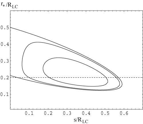
The condition for a wave propagating into the closed field lines. The contours (from innermost) correspond to closed field lines of ζ= 0.995, 0.999 and 1. The emission region is assumed to be on the last open field lines (ζ= 1). The dashed line represents the propagation path of a wave emitted at r*= 0.2RLC. The wave enters the CLFR at s= 0.04RLC and exits at s= 0.57RLC.
4.3.2 Fast pulsars
The fate of the radio emission that propagates into the CFLR is determined by the opacity (16). We consider PSR 1937+21 and the Crab pulsar. For PSR 1937+21, we have the mean flux density Sobsν≈ 240 mJy at 400 MHz and 16 mJy at 1.4 GHz. The brightness temperature times ΔΩ at RLC is estimated to be ΔΩTb∼1026 K and 5 × 10²³ K, respectively. The maximum depth from the last closed field line boundary is Δhmax≈ (r*+s)Δψ= (r*+s)3/2/(RLC−r*−s)1/2Δζ≈ 2.5 × 10⁻³RLC for r*+s= 0.5RLC, Δζ= 0.01. For P= 1.5 ms, one has Δhmax≈ 2 × 10² m. Using (17) and assuming B= 105 T and Δs= 0.2RLC, one finds rcr >RLC. The opacity at r∼RLC is τ∼53|ξp|2≫ 1 at ν= 1.4 GHz and it is even larger at a lower frequency. This implies that propagation in the CFLR is inhibited. Since both the leading and trailing components are visible, the emission must be produced at a radius where its trailing part does not propagate into the CFLR. From Fig. 3, this radius must be in the range r* < 0.13RLC or r* > 0.5RLC. Since the LC radius is only RLC≈ 7.2R0 and r* >R0≈ 0.14RLC, the only permitted radial range is r* > 0.5RLC. Alternatively, one may assume the radio emission occurs in a region away from the last closed field line surface, and in this case it propagates only in the OFLR. However, one needs to assume a two-pole model to explain the double peak feature.
For the Crab pulsar, the observed flux density is Sobsν≈ 950 mJy at 400 MHz and Sobsν≈ 14 mJy at 1.4 GHz, corresponding a spectral index α∼ 3.4. This gives ΔΩTb∼ 3 × 10²⁰ K for ν= 1.4 GHz at r=RLC≈ 1.6 × 10⁶ m and rcr∼ 0.5RLC |ξp|4/7. Since the propagation in the CFLR is nearly parallel, one has back scattering with |ξp|2∼n″2≫ 1. Since both the leading and trailing pulses are observed, the emission radius must be in the range r* < 0.13RLC or r*≥ 0.5RLC.
4.4 Constraint on backward emission
Induced three-wave processes impose a severe constraint on any model involving backward emission in the pulsar frame. Backward emission may be relevant for oscillatory gap models such as proposed by Levinson et al. (2005). In this model, pair cascades occur in an oscillatory manner sending secondary particles both forward and backward. This would lead to two photon beams propagating in opposite directions. Backward emission is also proposed for the interpretation of specific features of the pulse profile (Dyks et al. 2005). It is suggested here that the backward propagating waves must pass through the CFLR and undergo strong induced scattering. As the zeroth-order approximation, one assumes the photon beam is confined to the magnetic meridian plane, and ignoring both aberration and general relativity, one may estimate the radial distance to the crossing point (rc, ψc) from rc/cos (σ+ψ*) =r*/cos (σ−ψc). This gives
where ψ*≪ 1 is assumed, and π/2 −σ∼ 3ψ*/2. The polar angles ψc and ψ* can be expressed in terms of the relevant radii: ψc∼ (rc/RLC)1/2 and ψ*∼ (r*/RLC)1/2. On substituting them into (19), one finds the solution rc∼r*/4. When aberration is included, the propagation path of the backward emission bends towards the star in the corotating frame. A more rigorous treatment is outlined in Appendix A. Since for fast rotating young pulsars or fast millisecond pulsars, the critical radius rcr is close to or larger than the LC radius, propagation of the backward emission in the CFLR is not allowed. For example, as shown in Section 4.3, the Crab pulsar has rcr > 0.5RLC for n″ > 1. For the backward emission not to pass through the opaque region (r < rcr), the emission radius must satisfy r* > 4rcr > 2RLC. This implies that no backward emission can pass through the CFLR.
For a typical pulsar, the critical radius can be smaller than the LC radius. Pulsars that satisfy this condition (rcr < RLC) must have a period
Backward emission can propagate through the region rcr < r < RLC, provided that the emission is produced close to the LC, 4rcr < r* < RLC. We consider PSR B0950+08 as an example. It has a period P= 0.253 s and a magnetic field B≈ 108 T. We estimate ΔΩTb∼ 1017 K and rcr∼ 0.014RLCn″4/7. Backward emission can propagate through the CFLR if the emission region is at r* > 0.056RLCn″4/7. Note that n″ can be much larger than unity. For n″= 10, one has r* > 0.2RLC. Thus even for a typical pulsar, propagation of radio emission in the CFLR is strongly constrained and is allowed only in the region near the LC.
5 CONCLUSIONS
We consider the effect of induced three-wave turbulence on propagation of the radio emission in a pulsar magnetosphere. (As remarked in Section 2.5, this process is sometimes referred to, inappropriately we believe, as ‘stimulated Raman’ or ‘induced Raman’ scattering.) The low-frequency wave is either an electrostatic plasma wave propagating along magnetic field lines or an Alfvén wave propagating nearly along the magnetic field. We discuss both cases of propagation in the OFLR and CFLR. In the polar (OFLR) region, the induced processes strongly depend on the bulk velocity of the plasma and on the pair multiplicity (M). Since the scattering rate (cf. equation 13) decreases for increasing γ and M, the induced three-wave scattering effect on the propagation is suppressed due to the relativistic bulk flow (γ≫ 1) and M≫ 1. Assuming a modest bulk Lorentz factor γ∼102 and a multiplicity M∼102 for a young pulsar like the Crab pulsar, and γ∼105 and M∼10 for a fast millisecond pulsar like PSR 1957+21, we show that propagation of radio emission in the OFLR is little affected by the induced three-wave processes. An exception is the propagation of giant pulses. If the giant pulses are emitted relatively close to the star, they are subject to very strong induced processes that prevent them from escaping. The favoured region where induced processes can be effective is the transition region located at r*/γ from the source, where the photon beam propagates nearly perpendicular to the magnetic field in the rest frame. For giant pulses not to be completely destroyed by such processes, their emission region needs to be close to the LC. This conclusion is consistent with the conclusion reached by Romani & Johnston (2001) from a different argument, based on the alignment of giant pulses with the high energy emission.
Induced three-wave interactions are generally important for propagation of radio emission in the CFLR. Because the plasma in this region is stationary in the corotating frame, with |η| = 1, the processes are much more efficient than in the polar region. The induced three-wave processes are important throughout the CFLR except for pulsars with a relatively long period. We discuss three specific examples where the processes are relevant. (i) For the double pulsar J0737−3039B, we find that the processes discussed here are not efficient enough to explain the observed eclipse, due to the very low plasma density of the CFLR of pulsar B which has a relatively long period. However, the induced three-wave scattering can be effective if one assumes a density much higher than the GJ density (by a factor of 104). It is worth noting that a much higher plasma density is needed in the synchrotron/cyclotron absorption model as well (Lyutikov & Thompson 2005; Rafikov & Goldreich 2005). (ii) Our result imposes a strong constraint on the location of the emission region of pulsars with a pulse profile with widely separated leading and trailing components. There is a particular radial range where the trailing component may be swept into the CLFR due to aberration. (iii) Our result limits the visibility of backward emission. The backward emission must propagate through the CFLR where it can be dispersed due to three-wave interactions. For young or fast millisecond pulsars, the radius of the opaque region (where induced three-wave interactions are important) is comparable with or larger than the LC radius. In this case, backward emission may not be visible. For long period pulsars, the plasma density in the CFLR is low and the radius of the opaque region is smaller than the LC. The backward emission can propagate through the magnetosphere provided that it is produced sufficiently close to the LC and that its propagation path is outside the opaque sphere.
An important approximation made in our discussion is the strong magnetic field limit. Although such an approximation excludes the possibility of cyclotron resonance, our result should be valid for a finite, strong magnetic field. This is because the relevant frequency of the low-frequency waves (Langmuir and Alfvén modes) in the induced three-wave interactions considered here is much lower than the cyclotron frequency throughout the pulsar magnetosphere.
REFERENCES
Appendix
APPENDIX A: PHOTON BEAM IN THE COROTATING FRAME
In the non-rotating frame, a photon beam is assumed to be emitted at (x*, y*) in the field line direction and to propagate along a straight line described by

where s=ct/RLC=Ωt is the distance propagated in time t, σ is the slope of the photon beam and ± corresponds, respectively, to the forward and backward emission. Here, all the relevant radii, distances are in units of RLC. We consider an orthogonal rotator with a dipole field given by

where

is a parameter that specifies a particular field line, where ψd is the half-opening angle of the polar cap and ψB is the colatitude angle. The open field lines correspond to ψB≤ψd, that is ζ≥ 1. For a non-rotating dipole, one must have
To include the rotation, we consider a corotating frame in which the propagation path is described by
where R(s) =[X(s)2+Y(s)2]1/2=r(s), Ψ(s) =ψ(s) +s, and
The colatitude angle, radial distance of the emission point are Ψ(0) ≡Ψ*=ψ(0) ≡ψ*, R(0) =r(0) ≡r*. The tangent is
We use
At s= 0 we have
Since the derivation of (A9) is in the approximation to the order β=v/c, it can also be derived by a Galilean transformation. Assuming  , i.e. the tangent of the beam at s= 0 in the corotating frame, we obtain

The + sign corresponds to forward emission and − to backward emission. Due to the aberration effect, the photon beam must make an angle  to the field line in the observer's frame so that it is tangent to the field line in the corotating frame. We assume the magnetic field is a static dipole in the corotating frame:

where ζ= sin Ψd/sin ΨB. The tangent to the field line at s= 0 is
In the small angle approximation ψ*≪ 1, we have  and then (A11) reduces to

The photon beam direction at r* in the observer's frame advances in the rotation direction by r*.
For the trailing component, the condition for the forward propagating photon beam to cross the closed field lines with ζ≤ 1 is R=ζ2 sin2Ψ, where R(s) =r(s) =[x(s)2+y(s)2]1/2, that is

where tan ψ= (r* sin ψ*+s cos σ)/(r* cos ψ*+s sin σ). Note that the − sign corresponds to the backward emission propagating into the CLFR on the leading side. The condition is therefore that there exists at least a non-trivial solution to equation (A15) for s and ζ≤ 1 within the LC. In the case of forward emission, on approximating the left-hand side of equation (A15) by r*+s and using R(s) =r(s), one obtains the approximate form (18) after reversing them back to their dimensional form r*→r*/RLC, s→s/RLC. Similarly, the condition (A15) for the backward emission (the − sign) can be written approximately as r*−s≈ (ψ+s)2 in the small angle approximation, where ψ≈ (r*− 3sψ*/2)/(r*−s). One finds that the photon beam enters the CFLR on the leading side at a radius rc≈r*/4.
