


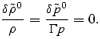
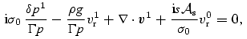
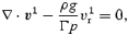
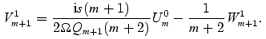
Abstract
We investigate the damping of neutron star r modes due to the presence of a viscous boundary (Ekman) layer at the interface between the crust and the core. Our study is motivated by the possibility that the gravitational wave driven instability of the inertial r modes may become active in rapidly spinning neutron stars, for example, in low-mass X-ray binaries, and the fact that a viscous Ekman layer at the core–crust interface provides an efficient damping mechanism for these oscillations. We review various approaches to the problem and carry out an analytic calculation of the effects due to the Ekman layer for a rigid crust. Our analytic estimates support previous numerical results, and provide further insight into the intricacies of the problem. We add to previous work by discussing the effect that compressibility and composition stratification have on the boundary-layer damping. We show that, while stratification is unimportant for the r-mode problem, composition suppresses the damping rate by about a factor of 2 (depending on the detailed equation of state).
1 INTRODUCTION
During the past few years, we have witnessed a renewed interest in neutron star oscillations. One trigger for the recent activity was the discovery that inertial modes in rotating fluid stars are generically unstable under the influence of gravitational radiation (a specific family of axial inertial modes, the so-called r modes, being the most relevant) (Andersson 1998; Friedman & Morsink 1998). Potential astrophysical implications of this instability have been extensively discussed in the literature, particularly in the context of gravitational wave observations (for a detailed review, see Andersson & Kokkotas 2001). Another motivation for work in this area is provided by the possible observations of crustal oscillations following magnetar flares (Israel et al 2005; Watts & Strohmayer 2006).
Soon after the discovery of the r-mode instability, it became clear that many additional pieces of physics need to be considered if one wants to draw ‘reliable’ astrophysical conclusions. Since much of the required physics is poorly, or only partially, known, this effort is ongoing. At the present time, the most important damping mechanisms that counteract the growth of an unstable mode are thought to be (i) viscous boundary layers at the core–crust interface (Bildsten & Ushomirsky 2000) and their magnetic analogue (Mendell 2001; Kinney & Mendell 2003), (ii) the bulk viscosity due to weak interactions in a hyperon core (Lindblom & Owen 2002; Nayyar & Owen 2006), and (iii) superfluid mutual friction due to scattering of electrons off the vortices in the neutron superfluid in the core (Mendell 1991; Andersson, Sidery & Comer 2006). At the same time, the mode amplitude is expected to saturate due to non-linear mode–mode coupling (Arras et al 2003; Brink, Teukolsky & Wasserman 2004). As the damping of unstable r modes could be an issue of astrophysical relevance, these mechanisms have attracted some attention.
At the time of writing, the available results indicate that for mature neutron stars the key damping agent may be the friction associated with the crust interface. The crust forms when the star cools below 1010 K or so, a few weeks to months after the star is born. Shortly after this, the heavy constituents in the core (neutrons, protons, hyperons) are expected to form superfluid/superconducting states. This leads to the suppression of, for example, the hyperon bulk viscosity (Haensel, Levenfish & Yakovlev 2002; Reisenegger & Bonacic 2003; Nayyar & Owen 2006) and the emergence of mutual friction. The estimates for superfluid mutual friction (Mendell 1991) indicate that, even though this mechanism may suppress the instability in the f modes completely (Lindblom & Mendell 1995), it is not very efficient for r modes (Lindblom & Mendell 2000).
We therefore focus our attention on the role of the crust, which as a first approximation can be modelled as a rigid spherical ‘container’ enclosing the neutron star fluid. Such configurations have been studied in several classic fluid dynamics papers (see the standard textbook by Greenspan (1968) for a detailed discussion of rotating fluids and a wealth of references). In the context of r-mode damping, the effect of a rigid crust was first discussed some years ago by Bildsten & Ushomirsky (2000), followed by the work of Andersson et al. (2000), Rieutord (2001) and Lindblom, Owen & Ushomirsky (2000). In this problem, the core fluid oscillations are damped because of the formation of an Ekman layer at the base of the crust and the associated Ekman circulation. The resulting damping is rapid enough to compete effectively with the gravitational wave driving of the r modes. Subsequent work by Mendell (2001) indicates that when a magnetic field is present in the Ekman layer the damping time-scale may become even shorter. Thus, the dissipation due to the presence of the crust–core interface plays a key role for the r-mode instability.
Our aim in this paper is to study the interaction between the oscillating fluid core and a rigid crust (using mainly analytical tools). A more refined model, which considers an elastic crust, is discussed in an accompanying paper (see also Levin & Ushomirsky 2001). Even though this problem has been discussed in some detail already, we have good motivation for revisiting it. It would be a mistake to think that the effect of the Ekman layer on an unstable r mode is well understood. While we may know the answer for the simplest model problem of a viscous fluid in a (more or less) rigid container, a number of issues remain to be investigated for realistic neutron stars. The presence of multiple particle species and the associated composition gradients may affect the Ekman circulation (Abney & Epstein 1996); the magnetic field boundary layer (Mendell 2001) depends strongly on the internal field structure (which is largely unknown) and whether the core forms a superconductor or not; once the core is superfluid, one would need to account for multifluid dynamics as well as possible vortex pinning, and so on. To prepare the ground for an assault on the latter two problems, we want to obtain a better understanding of the nature of the viscous boundary layer and the methods used to study the induced damping of an oscillation mode.
We will focus on the problem of a single r mode in the core (a slight restriction, but the generalization to other cases is not very difficult once the method is developed). In order for an analytic calculation to be tractable, a simple model for a neutron star is a prerequisite. Hence, we first consider a uniform density, slowly rotating, Newtonian star and reproduce familiar results for the Ekman problem. In doing this, we develop a new scheme which should prove useful in more complicated problem settings. Our study also serves as an introduction to boundary-layer techniques for the reader who is not already familiar with the tricks of the trade. We then compare and contrast the different methods that have been used to investigate the Ekman layer problem. This discussion serves to clarify the current understanding of the induced r-mode damping rate. Finally, we extend our analysis to compressible fluids with internal stratification. The results of Abney & Epstein (1996) for the spin-up problem suggest that both these features will have a strong effect on the Ekman layer damping. However, we prove this expectation to be wrong. For a toroidal mode, like the r mode, we find that stratification is irrelevant. The compressibility, on the other hand, does play a role but we demonstrate that the effect is much weaker than indicated by Abney & Epstein (1996). Rather than leading to an exponential suppression, the compressibility is estimated to reduce the r-mode damping by about a factor of 2.
2 FORMULATING THE EKMAN PROBLEM IN A SPHERE
As a first application of our boundary-layer scheme, we consider the Ekman layer problem in a spherical container. This is an instructive exercise as the solution to this problem is well known (Greenspan 1968). The so-called ‘spin-up problem’ forms a part of classic fluid dynamics and was studied in a number of papers in the 1960s and 70s. We found the work by Greenspan & Howard (1963), Greenspan (1964), Clark et al (1971), Acheson & Hyde (1973) and Benton & Clark (1974), particularly useful. The Ekman problem is also relevant for a discussion of unstable r modes. In fact, it is reasonable to expect that the associated r-mode damping time-scale is of the same order of magnitude as the spin-up time-scale in a rigid sphere, since an inertial mode has a frequency proportional to the rotation rate of the star, σ∝Ω.
In building a simple model of a neutron star with a rigid crust, we assume a core consisting of an incompressible, uniform density, viscous fluid surrounded by a rigid boundary. Furthermore, we work in a slow-rotation framework [which greatly simplifies the mathematical analysis as the star retains its spherical shape at  ]. Finally, we make the so-called Cowling approximation, that is, neglect any perturbation in the gravitational potential. These simplifications are obviously not necessary in a numerical analysis of the problem, but (in our view) the benefits of having an analytic solution far outweigh the value of a numerical solution to the complete problem. One can argue in favour of some of our assumptions, since most astrophysical neutron stars are slowly rotating (in the sense that their spin is far below the break-up rate) and the inertial modes which we are interested in are such that the density (and hence gravitational potential) perturbations are higher-order corrections.
Working in the rotating frame, our dynamical equations are the (linearized) Euler and continuity equations:


The enthalpy h, which is defined as

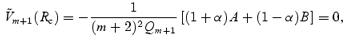
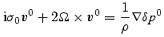
has been introduced for later convenience. In addition to the equations of motion, we have two boundary conditions for the core flow: (i) regularity at r= 0 and (ii) a ‘no-slip’ condition v (Rc) = 0 at the crust–core interface r=Rc. The role of viscosity is to ensure that the second condition is satisfied by modifying the inviscid solution in a thin boundary layer near the crust. This is known as the Ekman layer, and it has characteristic width  for typical neutron star parameters. Our aim in the following is to find a consistent solution to the problem when the solution in the bulk of the interior (the inviscid flow) corresponds to a singlel=m r-mode.
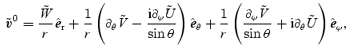
Schematically, we assume that the solution takes the following form [a standard uniform expansion in boundary-layer theory (Bender & Orzag 1978)]:

and similarly for the perturbed enthalpy δh and the mode frequency σ[we assume that all perturbations behave as exp(iσt)]:

The complex-valued frequency correction s is of particular importance, since its real part corresponds to the Ekman layer dissipation rate. The idea behind the expansion (4) is that the inviscid solution v0 is modified by  in the boundary layer in such a way that the no-slip condition is satisfied. This then leads to a change in the interior motion, represented by v1, which requires another boundary-layer correction
  and so on. In principle, this leads to an infinite hierarchy of coupled problems. In this picture, the various boundary/crust-induced corrections to the basic inviscid flow fall into two categories, namely boundary-layer corrections (always denoted by tildes in this paper) which are characterized by rapid (radial) variation [here
  ] and secondary ‘background’ corrections which vary smoothly throughout the star. Based on this different behaviour, when the expression (4) is inserted in equations (1) and (2), each of these equations splits into two components: one containing only boundary-layer quantities and another comprising the background quantities. These two families of equations are not entirely independent, since the boundary conditions communicate information between boundary-layer and background quantities.
Assuming that the solution to the inviscid problem takes the form of an axial r mode, we get
We also know that the l=m r-mode solution corresponds to a frequency

and can be expressed in terms of a stream function U0 as
where the phase is chosen for later convenience, and
(normalized to unity at the base of the crust).
The corresponding boundary-layer correction is a solution to

We also need to satisfy the continuity equation which leads to  , and
, and
Note that, we have only kept the highest radial derivative of the various variables in the boundary layer, and that, we have also neglected angular derivatives compared to radial ones. Finally, the solution to the  problem must be such that the no-slip boundary condition is satisfied, that is, we must have
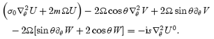
At the next level, we determine the change in the interior motion induced by the presence of the Ekman layer. This means that we must solve


together with the continuity equation

and a boundary condition

A solution to this problem should provide the frequency correction s, which encodes the rate at which the presence of the Ekman layer alters the core flow, that is, the induced damping of the r mode which we are interested in.
3 SOLUTION IN TERMS OF A SPHERICAL HARMONICS EXPANSION
So far, our calculation follows closely the standard treatment of the spin-up problem (Greenspan & Howard 1963; Greenspan 1968). At this point, we deviate by expanding the velocity components in spherical harmonics. We have several reasons for doing so. First, the standard approach (which will be reviewed in Section 4) leads to a boundary-layer flow that is explicitly singular in particular angular directions. Although one can demonstrate that this is not a great problem, and that the predicted Ekman layer dissipation can be trusted, it is not an attractive feature of the solution. We want to use an approach that avoids such singular behaviour. Secondly, the standard approach is somewhat limited in that it may not easily allow us to consider a differentially rotating background flow (or an interior magnetic field with complex multipolar structure). Our approach will allow such generalizations, should they be required.
3.1 The boundary-layer corrections
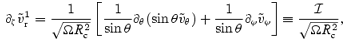
We first concentrate on the correction to the fluid velocity in the Ekman layer. We need to solve equations (13) and (14) and then determine  from equation (17). If we are mainly interested in determining the damping time-scale due to the presence of the Ekman layer, the induced radial flow will play the main role.
Assuming that  can be written as
that is, as a general decomposition into polar  and axial
  perturbations, and that our solution depends on ϕ as eimϕ, we get from equation (13)

Similarly, equation (14) leads to

We can combine these two equations to get
where
is the angular part of the Laplacian on the unit sphere.
If we now expand the various functions in spherical harmonics, that is,  etc., and then use their orthogonality together with the standard recurrence relations


where
we arrive at the two coupled equations
and
Since we know that we must match our solution to the inviscid r-mode solution at r=Rc, we now assume that all toroidal components apart from  vanish. Strictly speaking, this assumption is inconsistent. This can be easily seen by setting n=m→m+ 2 in the first of the equations above. In principle, one would expect an infinite sum of contributions. This problem is similar to that for an inertial mode in a compressible star (Lockitch & Friedman 1999). From a practical point of view, however, one must truncate the sum at some level in order to close the system of equations. Just like in the inertial-mode problem, one would expect the solution to converge as further multipole contributions are accounted for. This then provides a simple way to estimate the error induced by the truncation. Adopting this strategy, we will later compare our results to ones obtained by including more axial terms (
 and so on) in the boundary-layer flow.
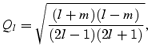
After setting n=m, we get (since Qm= 0):

and
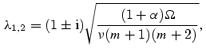
Using the standard ansatz  for a differential equation with constant coefficients, we can show that a solution will exist if
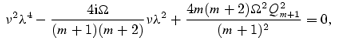
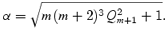
that is, for the two roots

where we have defined
The solutions correspond to eigenvectors
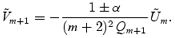
In order to satisfy the prescribed boundary conditions at the crust–core interface, we must have a vanishing velocity at r=Rc. Writing the solution as

where
we must have

Furthermore, we also require that
which leads to
Finally, we can use this solution together with equation (17) to determine  . Assuming that
  also takes the form (24), we readily find that
which can be integrated to give  . Hence, we have obtained all leading-order boundary-layer variables.
3.2 The induced interior flow
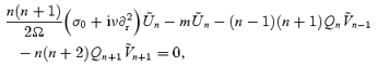
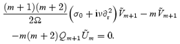
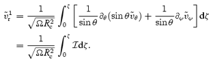
Having determined the appropriate solution in the Ekman layer, we now want to calculate the induced flow in the interior and deduce the damping rate of the r mode. By combining equations (19) and (20), and again using a solution of the form, equation (24) (albeit now without the tildes), for v1, we can show that we must have
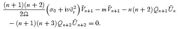
Expanding once again in spherical harmonics and using the fact that the right-hand side vanishes, unless l=m, we immediately arrive at

and a solution
Given this result, we can use the continuity equation to show that
(Note that the integration constant must vanish, since we would otherwise have a solution that diverges at the origin.)
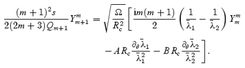
The final step in our analysis corresponds to combining equations (46) and (50) in such a way that
By integrating the two solutions, we find that
and
After combining these and reshuffling, we have
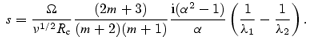
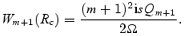
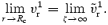
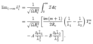
From the last equation, we can extract the damping rate,
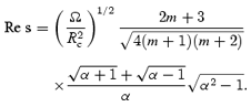
We also find that the frequency correction due to the presence of the Ekman layer is
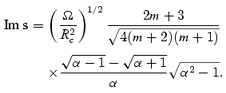
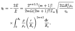
These expressions constitute the main new result of the first part of this paper. They have been derived by combining boundary-layer theory techniques with a decomposition in spherical harmonics. Putting numbers in, we find for m= 1 that s≈ 2.92 − 0.602 i. This should be compared to the results of Greenspan (1968) (see also Rieutord 2001), who found s≈ 2.62 − 0.259 i. The quantity which we are mainly interested in, the real part of s which gives the damping rate of the core flow, differs from Greenspan's result by about 11 per cent. This is not too bad, given that we truncated the boundary-layer solution at the level of a single multipole contribution. If we include further terms, we need to solve a system of equations larger than the ‘2 × 2’ problem given by equations (33) and (34). Including one more axial term  in the boundary layer, we end up with a ‘3 × 3’ problem and so on. As we include more multipoles in the description, our damping rate approaches Greenspan's result, cf. the results listed in Table 1. We see that if we consider the ‘4 × 4’ problem, we get results that agree with the standard ones, see the following section, to within 5 per cent or so. This is certainly much more accurate than our knowledge of the various neutron star parameters. It should be noted that, by solving the problem in a ‘non-standard’ way, we have learned an interesting lesson: in order to represent the boundary-layer flow accurately, we need to include a number of multipoles even though we have a very simple core flow.
Ekman dissipation rate s, computed in this work, compared with that of the standard approach in the literature (Greenspan 1968).
Ekman dissipation rate s, computed in this work, compared with that of the standard approach in the literature (Greenspan 1968).
4 THE STANDARD SOLUTION TO THE EKMAN PROBLEM
For completeness, and comparison with our calculation, we will now discuss the ‘traditional’ solution of the Ekman problem. This solution is described in detail in the paper by Greenspan & Howard (1963) as well as the book by Greenspan (1968) and is, essentially, a boundary-layer theory calculation without expanding in spherical harmonics. The formulation of the problem is identical to that described above.
By combining equations (13) and (14), we can easily show that we must have

Despite really being a partial differential equation, this is now viewed as a ‘constant coefficient’ ordinary differential equation for  as a function of r. The ansatz
  then leads to the indicial equation

which has solutions
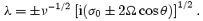
In order for the boundary-layer corrections to the velocity field to die away from the surface, we must have Re λ > 0. One can show that the two solutions that satisfy this criterion correspond to
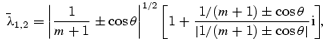
where we have (i) used the l=m r-mode frequency, and (ii) introduced  .
.
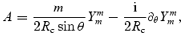
Given a solution for  , we find from equation (14) that

where the upper (lower) sign corresponds to λ1(λ2). The leading-order correction to the velocity field due to the presence of the Ekman layer can now be written as
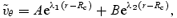

The coefficients A and B here should not be confused with those appearing in Section 3 (although in both cases they have similar roles). This solution needs to be matched to the inviscid solution in such a way that the no-slip condition at r=Rc is satisfied. Matching to the l=m inviscid r mode leads to
This completes the solution in the boundary layer. We want to infer the induced radial flow in order to estimate the Ekman layer damping of the core r-mode oscillation. The required relation is best expressed in terms of a ‘stretched’ boundary-layer variable
The  continuity equation then leads to
or
This is to be matched to the O(ν1/2) core solution in such a way that
Working things out for our boundary-layer solution, we find that
Using the induced core solution from before, that is, equation (53), we have

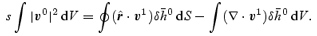
and we can determine the Ekman layer dissipation rate for the r mode from
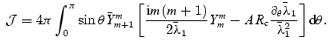
The final step is to use orthogonality of the spherical harmonics, that is, evaluate s from

where
The required integral can be much simplified if we use the symmetry of the integrand, see the discussion in Appendix A or alternatively Liao, Zhang & Earnshaw (2001). Thus, we get
The obtained values for the damping rate s are given in Table 1.
The solution to the Ekman problem described in this section is straightforward but somewhat limited, in the sense that it relies on the simplicity of equation (57). In a more general context, this approach may no longer be possible. Moreover, as we already pointed out, this solution exhibits a singular behaviour for certain angles (when λ= 0). From an intuitive point of view, one would clearly not expect a physical quantity, in this case the velocity field of the fluid, to exhibit singularities in certain angular directions. Hence, it is useful to discuss these singularities in more detail. To unveil the origin of the singular solution, we need to return to equation (1). Key to the boundary-layer approach was the assumption that the viscous term on the right-hand side is relevant only in a narrow region in the vicinity of (in our case) the neutron star crust. The idea is that the inviscid solution v0 is modified by a correction  in the boundary layer in such a way that a no-slip condition can be imposed. The boundary-layer corrections are characterized by rapid (radial) variation
  . Thus, neglecting the angular derivatives in the Laplacian in the right-hand side of the Navier–Stokes equation, we can derive equations (13) and (14). If we then conveniently ‘forget’ that we are actually solving partial differential equations and treat θ as a ‘constant’, then we arrive at equation (57). At the end of the day, the solutions we obtain are manifestly singular for particular values of θ. The problem stems from the assumption that the radial derivatives dominate the angular derivatives in the boundary layer. Without this assumption, we would have to solve the original partial differential equation, the standard approach to which is (of course) separation of variables via an expansion in spherical harmonics (as in our method in Section 3). However, given the singular solution derived above, it is very easy to show that

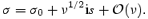
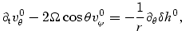
near the singular angular directions. Hence, this solution violates the assumptions made in the derivation which renders the calculation inconsistent. This argument shows that this solution is unphysical in the vicinity of these angular directions. Similar conclusions have been drawn by Rieutord & Valdettaro (1997) and Hollerbach & Kerswell (1995). They considered the complete problem numerically and showed that shear layers form in these specific angular directions. They also proved that the presence of these shear layers has a small effect on the damping rate. This is the key reason why both our method from Section 3 and the ‘exact’ singular solution derived above, where the detailed shear layers are neglected, lead to consistent and reliable estimates for the damping due to the Ekman layer. A comparison of the two velocity fields, cf. Figs 1 and 2, shows that the agreement is quite good away from the singular directions. Hence, it is not very surprising that the two calculations lead to similar estimates for the r-mode damping. It is worth noting that Hollerbach & Kerswell (1995) argued that the relatively slow convergence of the correction to the oscillation frequency, cf. Table 1, is due to the presence of the shear layers.
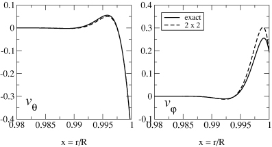
We compare the solution of the 2 × 2 problem (dashed line) to the standard ‘exact’ solution (solid line). The data correspond to parameters m= 2, E=ν/2ΩR2= 10−6, ϕ=π/3 and a typical angle θ=π/4. The two solutions are clearly in good agreement.
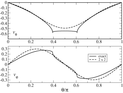
We compare the solution of the 2 × 2 problem (dashed line) to the standard ‘exact’ solution (solid line). The data correspond to parameters m= 2, E=ν/2ΩR2= 10−6, ϕ=π/3 and a distance away from the boundary given by  . The particular values of θ for which the standard solution is singular are apparent in this figure. However, away from these angles, we find the two solutions to agree well.
5 ANOTHER SOLUTION: SURFACE INTEGRAL APPROACH
There is yet another alternative for solving the Ekman problem, based on direct integration of the Euler equation. This approach is discussed in Greenspan's book (Greenspan 1968). With slight modifications, this method was used by Rieutord (2001) and Liao et al. (2001) in their studies of inertial modes.
Returning to equation (21), which determines the induced core flow, and reinstating the pressure and density instead of the enthalpy, we have
Multiplying by the complex conjugate  (the conjugate is denoted by a bar), and using the (conjugate of the) inviscid equation
as well as the continuity equation ∇·v0= 0, we obtain

Integration of this relation over the volume (V) of the star and the use of the divergence theorem gives
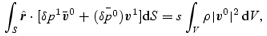
where S represents the surface at the core–crust interface. We know that the inviscid r-mode problem is such that

which means that we arrive at the final expression

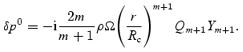
Now we can combine equation (82) with the matching condition for the induced flow, equation (69). This provides a connection to the calculation in the previous section. We can easily determine δp0 for the inviscid flow. From the r-mode solution to the velocity field, we find that
To determine the damping rate, we also need the volume integral (essentially the mode energy):
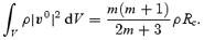
Putting all these ingredients together, we find that (using definitions from the previous section):
which is in agreement with the result, equation (73), of the previous section.
This final approach to the problem is obviously very elegant, and much less involved than the previous two calculations we have presented. Unfortunately, the surface integral approach relies on the assumption of incompressible flow. This assumption will not hold for stratified stars (Abney & Epstein 1996), see Section 7, or indeed stars with an internal magnetic field. Hence, we do not expect this method to be of much use for more complex (realistic) problem settings.
6 COMPARING DIFFERENT RESULTS
Before we move on to consider the more complex problem of a compressible star, it is meaningful to compare and contrast the different results for the Ekman layer damping of r modes in the current literature. Let us do this in chronological order. It was first suggested by Bildsten & Ushomirsky (2000) that the viscous boundary layer would provide an efficient damping mechanism. They estimated the associated damping rate by using the familiar plane-parallel oscillating plate result from Landau & Lifshitz (1987). Their result is not too far from the more detailed results derived in this paper, even though it does not account for the geometrical factors due to the sphericity of the star and the nature of the r-mode fluid flow. This is not very surprising since the geometric factors are of order unity as long as the thickness of the boundary layer is considerably smaller than the size of the star. At a local level, the boundary-layer flow is quite similar to that in the plane-parallel case.
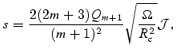
In his comment on these first estimates, Rieutord (2001) extracted equation (73) from Greenspan's work. As we have seen, this result has the relevant geometric factors etc., but it is based on a uniform density model. Lindblom et al. (2000) extended the standard method discussed in Section 4 to allow for non-uniform density models, and derived the boundary-layer-modified r-mode flow. Using the viscous shear tensor, they then arrived at the final result for the r-mode damping time-scale,
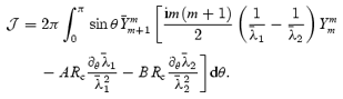
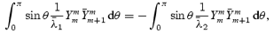
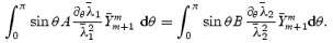
where ηc and ρc are the viscosity coefficient and the density at the core–crust interface, respectively, and  is an angular integral analogous to our
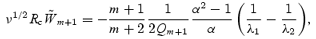
  . The integral on the right-hand side is essentially the kinetic energy of the r mode. In order to compare this expression to the result quoted by Rieutord, we should take ρ=ρc= constant and work out the radial integral. This readily yields equation (11) in Rieutord (2001). Hence, the two results are consistent, as they should be. To compare with our result, equation (73), we need to use the relation between the two angular integrals. One can show that
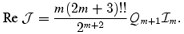
Given this relation, our result for the damping time-scale,
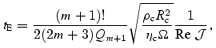
is also identical to Rieutord's result. From this comparison, it is clear that any difference between the various detailed studies of the Ekman layer problem in the r-mode instability literature is due to the chosen stellar model.
Quantifying the dependence of the damping rate on (say) the mass distribution in the star is obviously an important task. Lindblom et al. (2000) did this by performing calculations for a number of realistic supranuclear equations of state. Here, we will choose a more pragmatic approach, which we think provides some useful insights. Let us first return to equation (86), but instead of taking ρ=ρc we will, somewhat inconsistently, allow the two (constant) densities to be different. We then see that, in the case of the m= 2 mode,
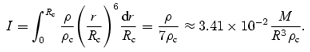
Now, compare this result to a star described by an n= 1 polytrope for which
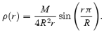
If we take ρc= 1.5 × 10¹⁴ g cm−3 and Rc/R≈ 0.85, which are fairly typical values according to table 1 in Lindblom et al. (2000), we find that
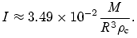
From this comparison, we see that one can quite easily bridge the difference between the constant-density calculation and the results of Lindblom et al. (2000). As a further exercise, one can work out the integral by combining the data in table 1 of Lindblom et al. (2000) for M, R and Rc with the n= 1 polytropic density profile. This leads to underestimates of the damping time-scale results obtained by Lindblom et al. for various equations of state by 10–30 per cent. This is due to the fact that realistic equations of state are slightly softer than the n= 1 polytrope. Nevertheless, it shows that the polytropic model captures the main features of the problem. One should keep in mind that the use of realistic equations of state for Newtonian neutron star models is dubious. For a given central density (say) the mass and radius often differ considerably from the corresponding results in general relativity. This means that it may not be entirely consistent to use realistic equations of state in the present discussion. On the other hand, it is important to get an understanding of how the results change with the stellar parameters, and over what range the damping time-scale for an unstable r mode may vary. We think that the above discussion led to some useful comparisons that provide useful steps towards this understanding. Possibly, the most important conclusion is that all current calculations are consistent.
7 INCLUDING STRATIFICATION AND COMPRESSIBILITY
So far, we have discussed the Ekman layer problem for incompressible fluids. Although this is not an unreasonable first approximation for neutron stars, it is well documented that both compressibility and stratification due to either temperature or composition gradients may be important. Considering also the results of Abney & Epstein (1996) for the spin-up problem, which suggest that the Ekman layer time-scale is significantly altered by both stratification and compressibility, it is clear that we need to relax our assumptions.
7.1 Formulating the compressible problem
We want to avoid the assumption of uniform density and include stratification and compressibility [while maintaining the calculation at  which means that the star is spherical]. In a perturbed compressible, stratified star, the equation of state is usually taken to have the form

where Δ represents a Lagrangian variation and Γ is the adiabatic index. Written in terms of Eulerian perturbations (δ) this means that, for our inviscid leading-order flow, we have
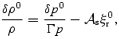
where the Schwarzschild discriminant is

(the primes represent radial derivatives). The Schwarzschild discriminant encodes information regarding composition gradients etc. (Reisenegger & Goldreich 1992).
The question now is, how does this more complex equation of state affect the boundary-layer calculation? At first sight, one might think that the answer will be quite messy. Fortunately, this turns out not to be the case. Let us first consider the inviscid flow discussed in Section 2. We then see that the introduction of the enthalpy was, indeed, a shrewd move. With the equations written in this way, we do not need to worry about the relation between the perturbed density and pressure, unless these variables are explicitly required. In our case, they are not. Thus, we swiftly prove that the inviscid r-mode flow remains unchanged for a compressible model.
The leading-order boundary-layer flow also requires little thought. As before, we find  . Given this, the remaining equations at this level are identical to those from the uniform density calculation. Hence,
  and
and  are obtained as in Section 3. Finally, from the equation of state, we find
The complications associated with stratification and compressibility enter the problem at the level of the induced core flow. Expressed in terms of the enthalpy, the Euler equations (19)–(21) remain unaltered, but the continuity equation is now given by
where we have preferred to use the perturbed pressure in order to emphasize the presence of the stratification. Inspection of the Euler equations, together with the fact that  , implies that
  and
and  . Hence, in the continuity equation, the second and third terms are
  , while the first term is of the order of
  . At the same time, the fact that we are considering an r-mode flow means that the last term is also
  . As we are working in the slow-rotation limit, we keep only the former terms, and we get
where g=p′/ρ. It is worth remarking that Abney & Epstein (1996) made similar assumptions in their analysis of the spin-up problem. At this point, we can infer that stratification has no effect (at leading order) on the Ekman damping rate of an r mode. This is in contrast to the situation for a general inertial mode (and the spin-up problem) for which the radial velocity component is of the same order as the angular ones. The last term in equation (96) must then be retained and stratification could be important. For our problem, this turns out not to be the case, which may be a bit of a surprise.
Our next task is to calculate the induced flow v1. Assuming the usual decomposition of the velocity field, we retain equation (49), that is,
At the same time, the continuity equation gives

where we have defined the dimensionless ‘compressibility’,

Combining these equations, we arrive at
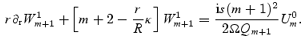
Once we solve this equation, we can replace equation (53) in the analysis of the incompressible case and infer the damping rate of the r mode. The problem is that, whereas the κ= 0 case is easily dealt with, the radial variation of κ in a realistic model will typically require a numerical solution.
7.2 Case study: the n= 1 polytrope
To get an idea of how important the compressibility corrections may be, we will consider the simple model problem of an n= 1 polytrope. Before doing this, let us make a few comments on the work of Abney & Epstein (1996). In their analysis of the spin-up problem, they arrived at an equation corresponding to equation (101). They then made the assumption that κ can be taken as constant. Since κ≫ 1 in the region of the boundary layer, the calculation simplifies considerably, and one easily shows that the compressibility leads to an exponential suppression of the Ekman layer damping. Working out the relevant algebra, we find a revised Ekman damping rate  given by

For canonical values m= 2, Rc= 0.9R and κ= 10 (see below), we would have

This suggests that the Ekman layer damping is strongly suppressed in a compressible star. In fact, if we take κ≈ 100 as in Abney & Epstein (1996), we would have a truly astonishing result where the boundary-layer dissipation was completely irrelevant. The analysis is, however, wrong.
To see what the problem is, we can work out κ for the polytrope (90). This leads to
where x=r/R and the last step follows from an expansion near the surface. As it turns out, this is a good approximation throughout the star. From this, we see that while κr/R is indeed large in the outer regions of the star (the divergence at the surface is due to the sound speed vanishing there), it vanishes at the centre and is certainly not large compared to m+ 2 in equation (101) in the inner regions of the star. This is relevant for our analysis, since we are trying to work out the induced flow in the core, not just the corrections in the thin boundary layer at the base of the crust.
Given the approximate expression for κ, it is straightforward to write down an analytic solution to equation (101). If we focus on the l=m= 2 r mode and express the right-hand side as B x3, then the solution is simply
This should be compared to the incompressible result W1inc=Bx3/7. Repeating the analysis following equation (53), we find that
This shows that the compressibility lowers the Ekman damping rate by a factor of 2 or so (for Rc/R= 0.9). Although this is far from irrelevant, it is certainly not as dramatic a suppression as the results of Abney & Epstein (1996) suggest.
The above analysis is, as far as we know, the first attempt to account for the effect of compressibility on the Ekman layer damping of r modes. We have shown how the problem can be solved (up to quadrature), and then estimated the magnitude of the effect for a polytropic model. Would it now be useful to consider an even more realistic model based on some tabulated equation of state? We think that the answer is no. There are two reasons for this. We have already discussed the well-known fact that one should be careful when using realistic (relativistic) equations of state in a Newtonian calculation, and that it is difficult to make sure that one is comparing like with like. A second reason why we feel that a more ‘detailed’ calculation may not be relevant is that we are still not considering the true physics problem. In a mature neutron star, we should incorporate both superfluid components at the crust–core interface and the magnetic field. We have shown that the Ekman layer damping in an incompressible normal fluid core differs from a compressible model by a factor of a few. This is typical of the uncertainties associated with (say) the equation of state, and is perhaps the level of accuracy that we should expect to be able to achieve.
7.3 Generalizing the surface integral approach
To complete our discussion of the compressible problem, it is relevant to consider how the surface integral approach discussed in Section 5 would have to be altered. Writing the Euler equations in terms of enthalpy, as in Section 2, instead of pressure, we have for the inviscid flow

Similarly, the  induced flow is described by

We have seen that  and
and  .
.
Repeating the steps described in Section 5, we obtain

The first three terms are  . The last term is much smaller,
  , and can therefore be neglected. Transforming the first integral to a surface integral in the standard way, we get at leading order,
This is the generalization of equation (82) for the case of a stratified and compressible fluid. The main difference from the incompressible result is the presence of the second term in the right-hand side. Since we know that, cf. equation (97),

we see that it encodes the dependence on the compressibility. Since it is a volume integral, it is also clear that the answer depends on the compressibility throughout the star, not just in the boundary layer.
8 SUMMARY
We have revisited the problem of the damping of neutron star r modes due to the presence of an Ekman layer at the core–crust interface. This problem continues to be of interest, since there is a possibility that the gravitational wave driven instability of the r modes is active in rapidly spinning neutron stars, for example, in low-mass X-ray binaries. The Ekman layer is known to provide one of the key damping mechanisms for these oscillations.
We reviewed various approaches to the problem and carried out an analytic calculation of the effects due to the Ekman layer for a rigid crust. Our obtained estimates support previous numerical results, and provide some useful insights into the problem. Of particular interest should be the discussion of the breakdown of the ‘standard’ solution to the problem associated with singularities in the velocity field in certain angular directions. Our comparison of previous results, which demonstrates that they are all consistent, is also useful.
We extended the analysis to include the effect of compressibility and composition stratification. This led to a demonstration that stratification is unimportant for the r-mode problem, but compressibility suppresses the damping rate by about a factor of 2 (depending on the detailed equation of state). The physical interpretation is that the compressibility counteracts the induced flow, and leads to a slightly less efficient energy transport away from the boundary layer. Our result corrects a similar analysis of Abney & Epstein (1996) for the spin-up problem (associated with pulsar glitches). By assuming that the compressibility can be taken to be constant, they predicted an exponential suppression of the Ekman layer damping. The reason why this assumption is not valid should be clear from our discussion.
To conclude, we think that this study clears the stage for work on more physically realistic models. The methods required to model Ekman layers in rotating neutron stars are now well understood. In particular, we understand the strengths and weaknesses of the different routes to the answer. In order to make our models more realistic, we need to account for the presence of both magnetic fields and superfluid components. The effects of magnetic boundary layers have been discussed by Mendell (2001) and Kinney & Mendell (2003). Their work shows that the magnetic field is of key importance. There are also many issues associated with superfluid neutron stars, ranging from the presence of additional dynamical degrees of freedom to novel dissipation mechanisms. It is clear that, while we have made progress on the simplest Ekman layer problems, many challenges remain.
This work was supported by PPARC through grant number PPA/G/S/2002/00038. NA also acknowledges support from PPARC via Senior Research Fellowship no PP/C505791/1.
REFERENCES
Appendix
APPENDIX A
In this appendix, we provide the steps needed to simplify the angular integral in Section 4. We need to work out
To do this, we use
and
In other words, we have
We can simplify this further in the following way:
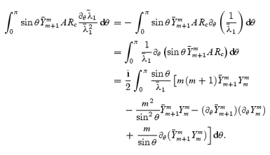
This way we arrive at equation (75) in Section 4.
